Fluid Dynamics & Materials Processing

DOI: 10.32604/fdmp.2021.014370

ARTICLE

Numerical Simulation of Turbulent Swirling Pipe Flow with an Internal Conical Bluff Body

Jinli Song1, Nabil Kharoua2,*, Lyes Khezzar1 and Mohamed Alshehhi1

1Khalifa University of Science and Technology, Abu Dhabi, United Arab Emirates
2National Polytechnic School of Constantine, Constantine, Algeria
*Corresponding Author: Nabil Kharoua. Email: nab2015ios@gmail.com
Received: 22 September 2020; Accepted: 11 February 2021

1  Introduction

Confined turbulent swirling flows are complex, highly three-dimensional, and unsteady. They are characterized by strong streamline curvature and turbulence anisotropy where the rotational component of the mean strain rate plays an important role. These flows take place in a broad range of industrial applications including fluid phase separation in cyclone separators [1], heat transfer rates enhancement in heat exchangers [2] and enhancing mixing in addition to flame stabilization in combustion burners [3]. In view of this, confined turbulent swirling flows have received attention within the academic and industrial communities. The related literature is rich in experimental and numerical studies. However, the simulation of such flows, using RANS-based turbulence modelling is still a challenging task. This work represents a contribution towards assessing such models for a three-dimensional turbulent swirling pipe flow which encounters a blockage of conical shape. This particular geometry possesses features of swirling multiphase pipe flow occurring in in-line separators [4]. This separator is equipped with a novel type of swirlers consisting of multiple radial cylindrical holes inside a hollow cylinder.

Confined turbulent swirling flows and their evolution in long pipes were studied by [5–9] where swirl was generated by stationary swirlers or rotating pipes. Studies of flows in the near field past expansions include those of [10–13]. In their study, Pashtrapanka et al. [9] found that a swirling flow in a pipe can lose its axial symmetry along the downstream direction. They suggested that calculations for swirling pipe flows should be done with a three-dimensional model to capture their complex features.

Numerical simulations of turbulent swirling pipe flows have been conducted by several authors using a variety of RANS turbulence models that ranged from the two-equation family to the full Reynolds stress models. The encompassing study of Jakirlic et al. [14] used the standard k-ε model and its low-Reynolds-number extension, three variants of the full Reynolds stress model (RSM). The RSM variants are: The basic high Reynolds number version, the model of Speziale et al. [15] and a low Reynolds number version of the RSM. This particular study permitted to highlight several important points: (i) The standard k-ε model fails to replicate important features of the flow resulting in solid body rotation which was also observed previously [16,17], (ii) The low-Reynolds number version of the RSM was superior since it is able to mimic stress anisotropy in the near wall region, (iii) The wall function approach is unsuitable for strong swirling flows driven by near wall phenomena such as in rotating pipes or if transition is present (iv) Whereas if the extra strain rates, responsible for non-equilibrium effects, arise from the inner part of the flow as in swirling flow entering pipes and if the bulk Reynolds number is high the wall function concept can provide a reasonable alternative for modeling the near wall region. Brennan [18], in his study of swirling flow in cyclonic separators, found that the RSM model, with its linear and quadratic pressure strain correlations, predict almost identical velocity profiles. Erdal et al. [19] simulated a 3D swirling flow with different turbulence models in a cylindrical cyclone. The simulations captured the general trend of the experimental data. The simulation with the standard k-ε model predicts higher rotational flow and RSM predicts a much stronger decay of tangential and axial velocities. Wegner et al. [3] evaluated the performance of Unsteady Reynolds Averaged Navier-Stokes (URANS) models in predicting an unconfined swirling flow with Precessing Vortex Core (PVC). The swirl number was 0.75 and Reynolds number was in the range 10,000–42,000. The URANS results showed good agreement of mean velocities with experimental data. Ramirez et al. [20] simulated an unsteady single-phase turbulent flow in a swirl combustor using the standard k-ε and the Reynolds stresses models. Both models predicted a complex asymmetric flow with PVC and inner recirculation zone. The prediction via RSM was more realistic with a lack of flow symmetry and periodicity exhibiting stronger and persistent vortical motions. Large eddy simulation (LES) was used by Kharoua et al. [4] for the same geometry of the present study with and without a bluff cone. LES was able to predict the presence of the peak in the r.m.s of the axial and tangential velocity components.

Advanced turbulence models such as LES or direct numerical simulation (DNS) can perform better than RANS models for such flows but remain prohibitively expensive especially for industrial-type configurations which have usually flow passages of complex three-dimensional nature, see [4]. Complex three-dimensional geometries encountered in industrial applications are demanding in terms of meshing and turn-around time for design. In addition, what-if scenarios simulations are usually excessively expensive.

The present work aims to elucidate the behavior of confined swirling flow inside a short pipe which encounters a downstream blockage of conical shape. It is important to mention that the geometrical configuration considered herein is meant to mimic an innovative gas-liquid separator in a simplified way. This is meant to be a first step to evaluate the ability of CFD to mimic the flow features of single phase swirling flow in the simplified configuration with a conical bluff body before extending the work later on to two-phase flows. In order to obtain meaningful simulations, the complex three-dimensional swirler geometry is also included in the simulation domain. Different RANS-based turbulence models are used. Numerical results were benchmarked with experimental data obtained using Laser Doppler Anemometry in addition to LES simulations conducted by the same research group [4,21–25]. Since the geometry is extracted from that of a two-phase separator, additional parametric simulations are conducted to study the influence of Reynolds number on flow and swirl decay. It is to be noted that numerical studies on confined turbulent swirling flows interacting with a bluff body in the literature are limited to disk bluff bodies [26,27].

Section 2 of this work presents the simulation approach used, while the results are discussed in Section 3 followed by conclusions in Section 4.

2  Numerical Simulation Approach

The flow is assumed incompressible, turbulent and three-dimensional, under steady and unsteady conditions. The mathematical formulation is presented first followed by the computational domain configuration, the boundary conditions and the numerical assumptions.

2.1 Mathematical Model

The flow is governed by the Reynolds-Averaged Navier-Stokes equations. The continuity and momentum conservation equations in Cartesian tensor notation are given by:

∂∂xi(ρui)=0 (1)

∂∂t(ρui)+∂∂xj(ρuiuj)=−∂p∂xi+∂∂xj[μ(∂ui∂xj+∂uj∂xi)]+∂∂xj(−ρui′uj′¯) (2)

The Reynolds stresses −ρui′uj′¯ require a turbulence model in order to close the above system of equations.

2.1.1 Reynolds Stress Model

The Reynolds Stress Model (RSM), solves the transport equations for each term of the Reynolds stress tensor, it is recognized to give the best performance among RANS models for highly swirling flows. The exact transport equations of the Reynolds stresses, ρui′uj′¯ , may be written as follows:

∂∂t(ρui′uj′¯)+∂∂xk(ρukui′uj′¯)=−∂∂xk[ρui′uj′uk′¯+P′(δkjui′+δikuj′)¯]+∂∂xk[μ∂∂xk(ui′uj′¯)]−ρ(ui′uk′¯∂uj∂xk+uj′uk′¯∂ui∂xk)+P′(∂ui′∂xj+∂uj′∂xi)−2μ∂ui′∂xk∂uj′∂xk¯ (3)

The term on the left side of the above equation represents the local time derivative and convective term, and the terms on the right hand side represent the turbulent diffusion, molecular diffusion, stress production, pressure strain and dissipation, respectively. The stress transport equations solved are naturally the modelled equations which are well documented in the literature. In this study, we use the Linear Pressure-Strain Model. The pressure-strain term, ∅ij , is modeled according to the proposals by [28–31].

2.1.2 RNG k-ε and SST k-ω Model

The two-equation turbulence models (k-ε and k-ω) are based on the Boussinesq hypothesis to model the Reynolds stresses:

−ρui′uj′¯=μt(∂ui∂xj+∂uj∂xi)−23(ρk)δij (4)

This method requires low computational cost but is based on the assumption of an isotropic turbulent viscosity μt .

In the RNG k-ε model, two transport equations, for the turbulent kinetic energy k and its rate of dissipation ε, are solved. The model equations were derived using a statistical technique called renormalization group theory [32]. Compared to the standard k-ε model, it has an additional term in the dissipation rate equation that improves the accuracy for rapidly strained flows and a modified turbulent viscosity to account for the influence of swirl.

The Shear-Stress Transport SST k-ω model [33] accounts for the transport of the turbulence shear stress in the definition of the turbulent viscosity. It is more accurate and reliable for a wide class of flows (for example, adverse pressure gradient flows, airfoils, transonic shock waves) for which the standard k-ω model is weak. Further details can be found in fluent documentation [32].

2.2 Numerical Method

2.2.1 Geometry and Meshing

The computational geometry used in this study is inspired from a new type of liquid-gas separator. A Perspex pilot model is shown in Fig. 1. The separator uses the centrifugal effects of the swirling flow to separate the phases. The simplified geometry, defining the flow domain, is presented in Fig. 2 with the coordinates system considered. It consists of a short inlet pipe of inner diameter 41 mm connected the swirl cage (Fig. 2a). The swirl cage is a short cylindrical housing of length 94 mm and diameter 150 mm. The swirler, shown in Fig. 2b, is made of a stainless steel cylinder concentrically inside the swirl cage housing. It contains sixty radially inclined holes of 4 mm diameter divided into six rows of 10 holes each. The swirl cage generates a swirling flow which extends into a straight pipe of 610 mm length and 41 mm diameter. At the end of the pipe, the swirling flow interacts with a conical bluff body containing three kidney shaped openings representing the outlet of the computational domain (Fig. 1c).

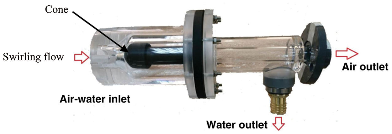
Figure 1: Pilot Perspex model of the in-line separator (swirl cage removed)

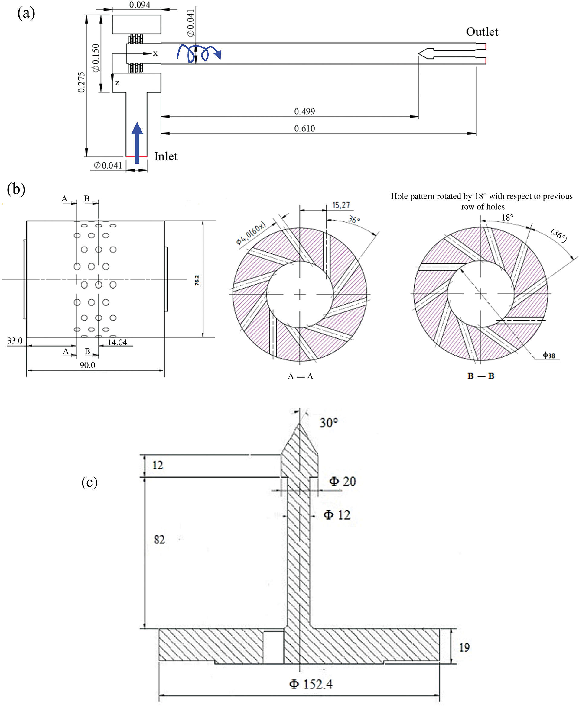
Figure 2: (a) Geometry of flow domain, (b) Swirler, (c) Bluff body

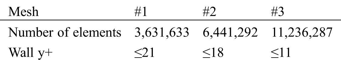
The hexahedral grid was generated using ANSYS Workbench. Different computational grids were used as illustrated in Tab. 1. Attention is directed towards the resulting swirling flow which takes place between the swirler outlet and the tip of the bluff body.

Table 1: Computational grids

2.2.2 Boundary Conditions

An inlet velocity condition was used while a constant pressure (zero gauge pressure) was prescribed at the outlet. A no-slip condition was taken for the remaining boundaries.

2.2.3 Numerical Tools and Simulation Strategy

The commercial software Fluent 17.1, based on the finite volume method, was used in this study. The calculations were executed under steady conditions for all turbulence models. In addition, unsteady calculations were performed with the SST k-ω and RSM models to investigate the effect of steady assumption. Water was the working fluid under atmospheric pressure and ambient temperature. Concerning the near-wall treatment, ANSYS FLUENT accounts for the variability of the mesh resolution near the wall by blending different wall-treatment approaches so that each approach is employed locally based on the local values of y+. In the present study, y+ reached low values close to unity at some regions of the computational domain allowing for the sub-layer to be directly computed while, at some other regions, y+ reached higher values (Tab. 1) necessitating the use of wall functions.

The pressure-velocity coupling is achieved by using the SIMPLE scheme. For SST k-ω and RNG k-ε models, the pressure was discretized using second order upwind scheme while the RSM model uses the PRESTO! Scheme. The discretization of the convective terms for momentum, turbulent kinetic energy, dissipation rate and Reynolds stresses is achieved by second order upwind scheme.

During the simulation for the unsteady case, the mean axial and tangential velocity and static pressure from two points at different axial positions within the outlet pipe are used for monitoring purposes. Convergence is assumed when the monitoring data achieve a statistically steady state. The transient simulation is conducted in three steps. First, a steady solution with same settings is launched to generate a good initial instantaneous field for the transient simulation. After that, the transient simulation was run to allow the instantaneous field to develop with a time step equal to 4 × 10-4 s. Finally, the time-averaged field was monitored at the abovementioned points until statistical convergence is reached. It is important to mention that the residence time of the flow, based on the axial bulk velocity of 1 m/s and the length of the computational domain, was 0.81 s. For stability purposes, the Courant Number was kept smaller than unity. The time integration was based on the second order implicit scheme. After 3 s of physical flow time, data collection, was performed during 2.76 s of flow time.

3  Results and Discussion

The base case flow corresponds to a Reynolds number based on the bulk velocity and pipe diameter of 41,000. The test fluid was water at room temperature. Grid independency tests are considered first. Subsequently, a comparison of performance between the turbulence models considered in this study is conducted primarily against experimental data of [21,22] and accessorily with LES computational results of [4]. It has to be stressed that the LES results were obtained with a very fine grid and involved considerably more usage of computational time. The quantitative comparison uses the mean axial and tangential velocity components, their corresponding normal turbulent single point correlations and the cross correlation between the axial and tangential components of the fluctuating velocities and the swirl number axial evolution. The third subsection examines the effect of varying the Reynolds number on the mean flow quantities such as axial and tangential velocities and swirl number.

3.1 Validation and Grid Refinement Study

Grid independency tests were conducted using the RSM model due to its superiority. The Reynolds number, in the pipe, was equal to 41,000 corresponding to available experimental results. Three meshes of 3.6, 6.4 and 11.2 million cells were used. Fig. 3 compares the mean axial and tangential velocity profiles for the three meshes at an axial location x/D = 10. It can be seen that grids 2 and 3 perform similarly with slight differences. The results for mesh 1 are quite different and fail to replicate certain important flow features such as the central reverse flow region and the Rankine vortex flow structure. The estimated wall y+ values inside the outlet pipe and around the bluff body surface, for the meshes considered, are illustrated in Tab. 1. As a compromise between accuracy and computational cost, Mesh #2 is used for the simulation of the cases considered in this work. It is inherently assumed that the use of the RSM as the main model used for grid convergence test will not invalidate this conclusion when the other models are used. It is worth mentioning here that the mesh attempts to capture all the details of the three-dimensional geometry. It therefore includes the swirler with its intricate flow passages in the solution domain and the resulting three-dimensional structure of the flow. Thus, it tries to conduct an evaluation at industrial scale under RANS framework of modelling.

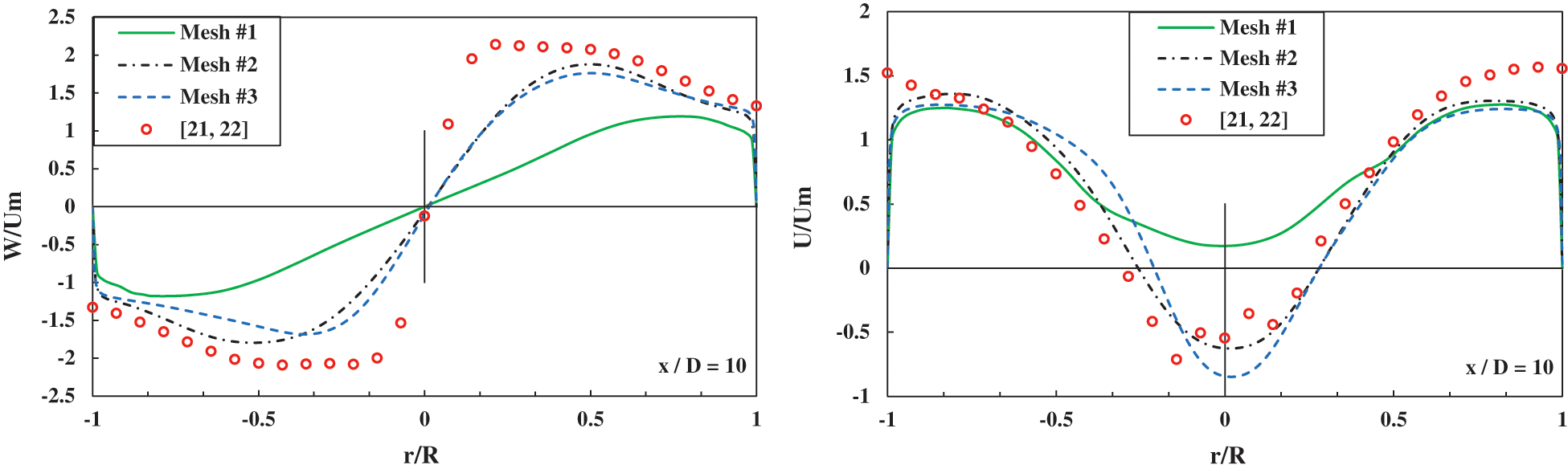
Figure 3: Radial profiles of the mean axial and tangential velocities for different meshes at x/D = 10

3.2 Mean Velocities and Reynolds Stresses and Swirl Number

The radial profiles of the mean axial and tangential velocities, at three representative axial positions, are compared with experimental and LES data as shown in Fig. 4. The simulation using RNG k-ε model is performed in a steady state mode while the simulations using other models are conducted under both steady and unsteady states. The LES profiles of reference [4] are added for comparison.

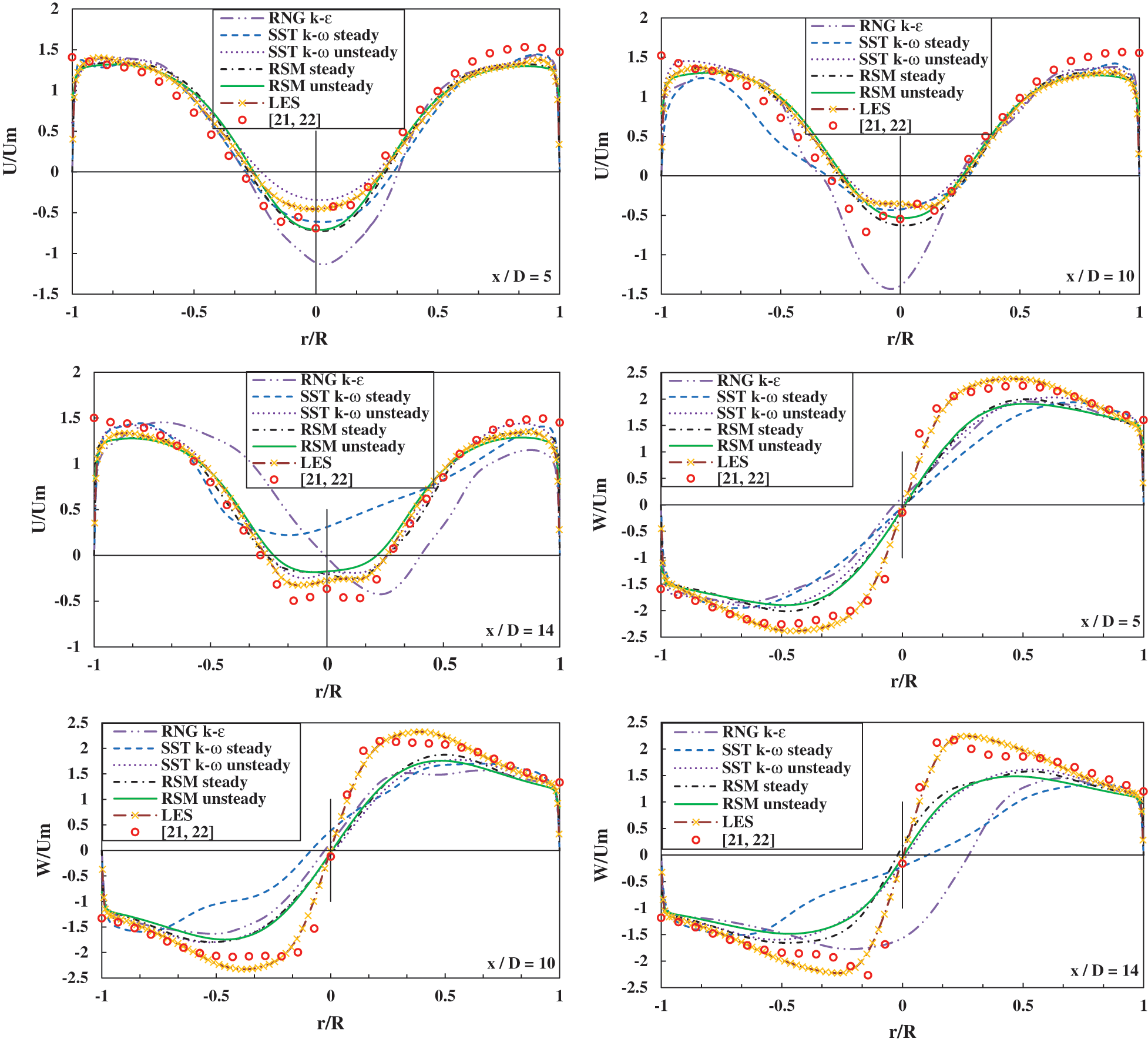
Figure 4: Radial profiles of the mean axial and tangential velocities

Steady and unsteady RSM simulations predict similar results suggesting that a steady RSM simulation is sufficient to avoid a costly unsteady RSM simulation if not specifically needed. The mean axial velocity profiles show that the central core flow reversal, which plays an important role in a phase separation, is predicted with a relative accuracy using the RSM model. The reversal flow persists from the exit of the swirl cage till the bluff body. The SST k-ω and RNG k-ε, under steady conditions, fail to capture the mean axial velocity profile which loses symmetry starting from x/D = 4. The reason behind this remains unclear. The mean axial velocity remains under-predicted by RSM in the annular region near the wall, by as much as 50%.

The profiles of the mean tangential velocity correspond to a Rankine vortex. As the flow proceeds downstream, the mean axial and tangential velocities decay due to viscous dissipation. The peak tangential velocity shifts towards the pipe axis which is consistent with previous findings [34]. The RNG k-ε and steady SST k-ω simulations exhibit a strong asymmetry in the velocity profile at x/D = 10 and x/D = 14. Similarly, the results of unsteady SST k-ω simulations show a noticeable improvement compared with steady SST k-ω simulation. All the RANS and URANS simulations fail to capture the mean tangential velocity peaks in contrast with LES results of [4]. In particular, all RSM calculations display a lower solid body rotation than the experiments inside the core and hence suggest that the calculated swirl intensity is decaying faster than the experimental one.

In swirling pipe flows, the profiles of the normal turbulent stresses exhibit larger peaks at the center and are highly anisotropic compared with uni-directional conventional pipe flows. For this reason, the radial profiles of the axial and tangential Reynolds stress components at three representative axial positions are shown in Fig. 5. The presented results are limited to RSM, experiments and LES [4]. The RSM model fails to capture the peak along the axis of the pipe, in the core region. Similar behavior was also obtained in the computational work of highly swirling flows in combustors investigated by [35]. They concluded that the inadequate modeling of pressure strain, especially its rapid part, is responsible for the inaccurate prediction of Reynolds stresses. It is well known that the model coefficient could be adjusted to improve the results but the approach remains customized and not universal. The LES simulation predicts the turbulence, at the core, in a better way although still exhibiting important discrepancies suggesting that model and mesh-resolution tunings are required in the core region due to this complex flow behavior. Outside the core region the levels of the normal stresses remain in qualitative agreement. The same can be said for the shear stress component also shown in Fig. 5.

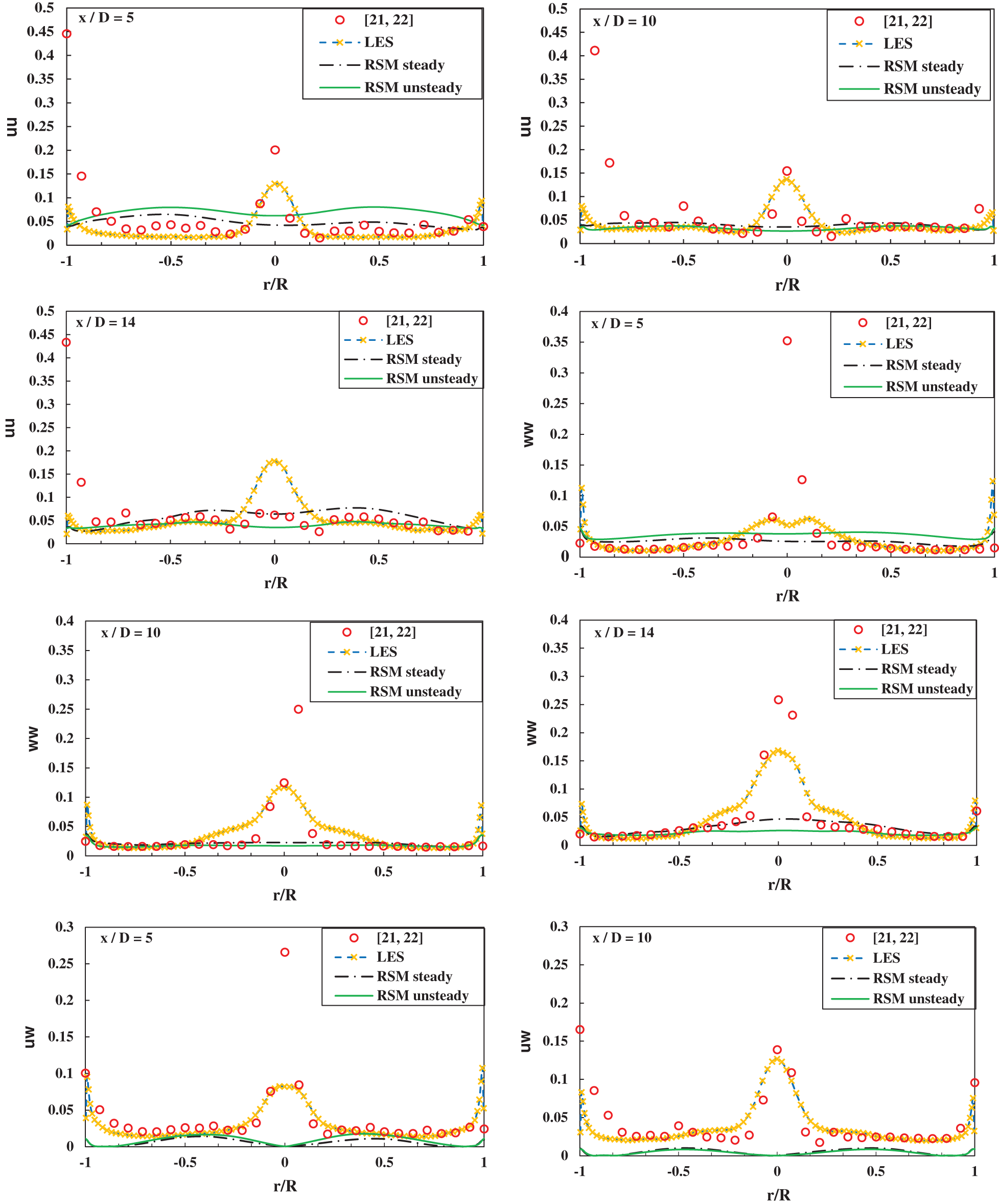
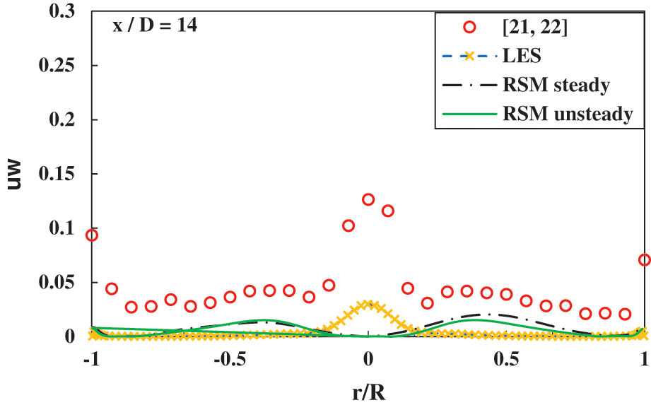
Figure 5: Radial profiles of Reynolds stresses for different turbulence models

The swirl number is a non-dimensional number that is used to characterize the intensity of swirling flows, which for a pipe of radius R can be expressed as, see [5]:

S=2∫0Rr2UWdrR3Ub2 (5)

where Ub is the bulk velocity inside the pipe. To calculate S, a numerical integration is necessary to evaluate the numerator. It is assumed that the velocities vary linearly between the closest measured velocity to the wall and the zero value at the wall itself.

The swirl number variation along the axial direction within the pipe is shown for the RSM model and experimental data in Fig. 6.

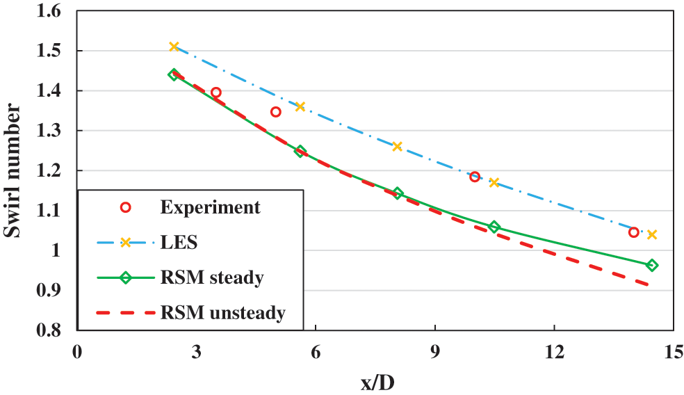
Figure 6: Swirl decay for different turbulence models, experimental values from [21,22]

Results from the two-equation turbulence models are not shown since they failed to capture, accurately, the variation of the fluid velocity along the pipe at least with the present mesh used. The RSM model captured the swirl decay trend correctly although with a quantitative discrepancy of about 10%. This is due to the fact that swirl intensity was under-predicted by RSM as shown with the mean tangential velocity. The swirl intensity depends on an accurate prediction of the tangential mean velocity profile which, in turn, depends on the flow structure inside the swirler holes. The control of the swirling flow characteristics necessitates a meticulous parametric study on the complex geometrical details of the present swirl generation technique.

Fig. 7 depicts the mean axial and tangential velocity profiles for the cases with different inlet Reynolds numbers at three representative axial positions within the long pipe. The numerical results and discussion are confined to the RSM simulations. Each velocity profile is normalized by the bulk axial velocity for the corresponding axial position. For Re = 4,100, the reversal flow disappears at x/D = 6 and the width of the forced vortex is the smallest among all the cases. Beyond x/D = 6, the flow has a positive axial velocity similar to unidirectional pipe flow. This type of flow indicates possibly a vortex breakdown phenomenon. For Re = 20,500, the width and magnitude of the reversal flow decreases along the pipe axis until it disappears at x/D = 14 just upstream of the tip of the bluff body. The most intensive reversal flow is obtained when Re = 41,000. The peak tangential velocity in the annular region increases with Reynolds number. It is to be noted that for Re = 4,100, after the disappearance of the core reverse flow, the flow exhibits a solid body rotation distribution, yielding an almost uniform positive axial velocity. Parchen et al. [36] have demonstrated how the axial velocity distribution, in swirling pipe flow, can be influenced by the swirl generator geometry. Consequently, in some cases, the central reverse flow can be eliminated. In the work of Pashtrapanska et al. [9] no reverse flow region was measured due to the swirl generator geometrical structure.

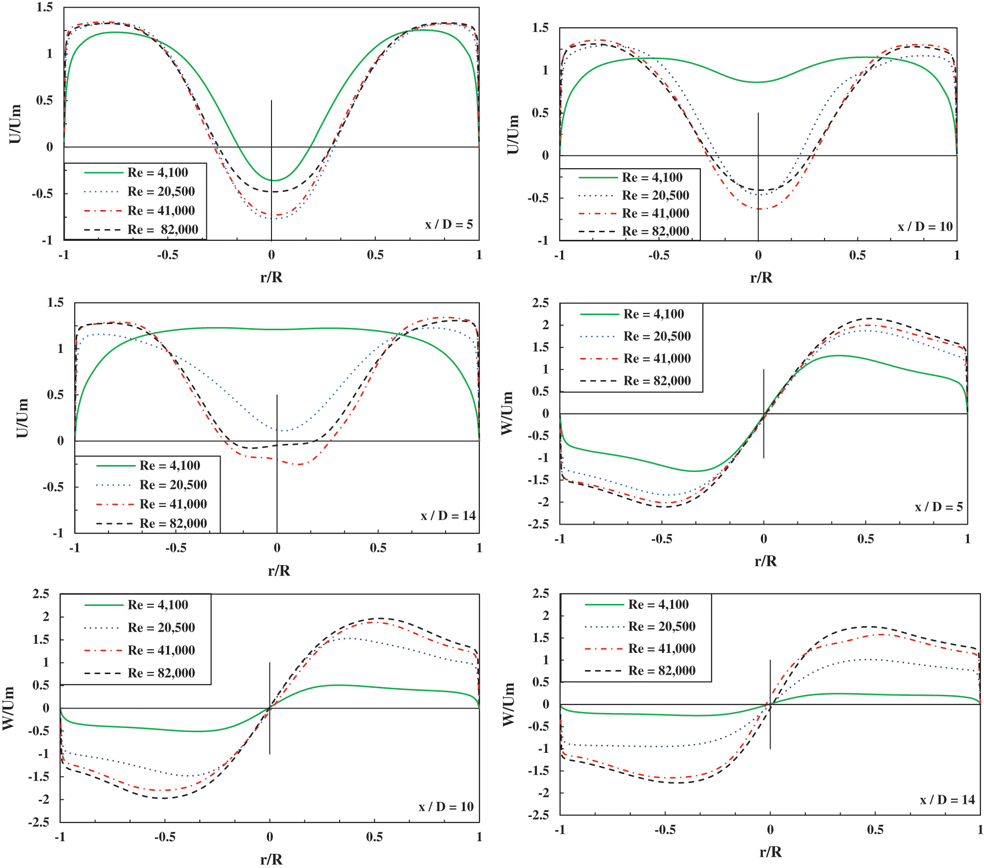
Figure 7: Radial profiles of the mean axial and tangential velocities for different Reynolds Numbers

Swirl decay prediction for swirling pipe flow is relevant to several engineering applications [8] including flow inside two-phase separation equipment. It is, therefore, important to consider the influence of the Reynolds number on it. At this point, it is fit to point out that several researchers have obtained an expression for the variation of swirl number with axial distance in a pipe [8,37]. Thus, by integrating the momentum equation in cylindrical coordinates and assuming slowly developing flow along the axial direction, neglecting turbulent shear stress and assuming relatively low swirl intensity the swirl number is shown to vary as:

SSr=e−β(x−xr)D (6)

where Sr is the reference swirl number at a reference axial position xr.

The present discussion will be limited to cases when Re > 4,100 where the flow exhibits a tangential velocity profile of the Rankine type. The calculated values of β were 0.058, 0.033 and 0.027 for Reynolds number values of 20,500, 41,000 and 82,000, respectively. These values are in agreement with the findings of Najafi et al. [37] stating that β decreases almost linearly with Reynolds number. In addition, Steenbergen et al. [8] have generated a comprehensive graph encapsulating the variation of the decay rate of swirl β with Reynolds number for a set of previous experimental studies performed in the period from the 1960’s till 1998. The results cover a wide range of swirl generation methods and swirl intensities. The graph confirms the exponential nature of the decay rate. Despite a relatively wide scatter, depending on the swirl number ranges and exact experimental conditions, it remains, however, a very useful reference for smooth pipes. The present results agree very well with the values reported in that graph. Thus the value of β for Reynolds of 20,500, 41,000 and 82,000 agree very well with the findings of [5,38,39], respectively. The value of β = 0.033 for a Reynolds number of 41,100 compares reasonably with the experimental value of [8] for the closest value of the Reynolds number equal to 50,000.

This information is crucial when considering the optimum axial position of the bluff body inside the real gas liquid separator.

Fig. 8 depicts the pressure distribution on the bluff body surface for different inlet Reynolds numbers. It illustrates the effect of the swirling flow, with different swirl intensities (shown in Fig. 9), on the loads experienced by the bluff body. For the case with Re = 4,100, the pressure peak is observed on the bluff body apex. It means the stagnation point is at the cone apex for low swirl since the flow, for this Reynolds number, has no reversal in the downstream direction along the axis. Increasing the Reynolds number (swirl intensity) causes flow reversal on the axis and the apex to become gradually a region with a depression. On the other hand, the cylindrical surface of the bluff body undergoes a maximum pressure. The implication for phase separation is that the central depression, is necessary to drive the lighter phase towards the core region while the heavier phase is ejected outwards under the centrifugal force effects. Thus, it is very important to consider the swirling flow characteristics when investigating the optimal design of the bluff body in terms of size, shape and location for a more efficient separation.

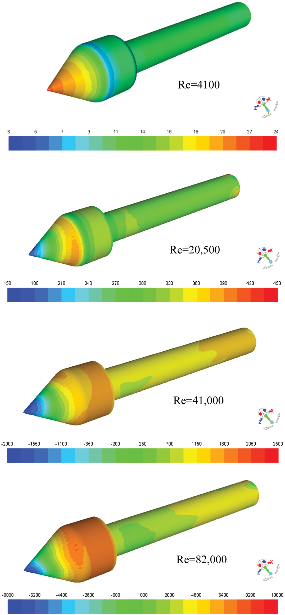
Figure 8: Pressure (Pa) contours on the bluff body surface

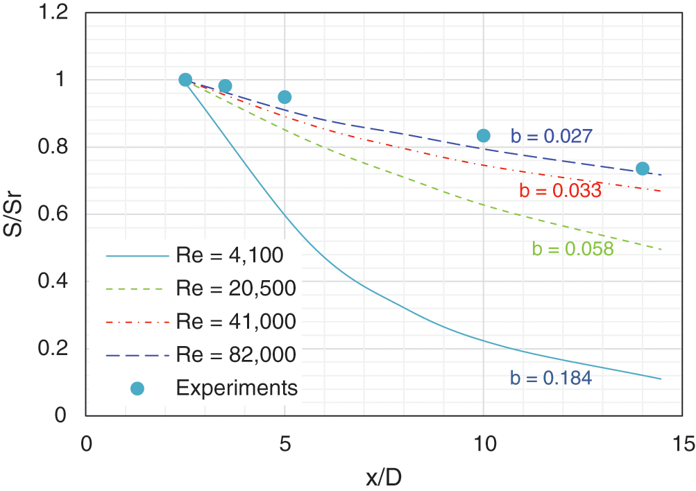
Figure 9: Swirl decay for different Reynolds numbers, experiments from [8]

It is worth mentioning that the hollow cone would undergo a negative drag force, for high swirl numbers, tending to dismantle it from its supporting hollow tail pipe. Obviously, more research work is necessary to investigate this effect in detail.

4  Conclusions

A numerical study of turbulent swirling flow interacting with a conical bluff body, inside a short pipe, was conducted. The present simulations considered the details of the geometrical configuration including the complex swirl generator. The following conclusions can be made:

The RSM turbulence model exhibits the best performance among the RANS-based models used in this study. The RNG k-ε and SST k-ω in steady mode failed to predict the important features of the flow. The SST k-ω model, in unsteady mode, could relatively improve the accuracy of the results but remained inferior compared to the RSM model.

The RSM, in both steady and unsteady modes, performed equally well and provided the best performance in the sense of being able to capture the variation of the mean axial and tangential velocity profiles and swirl decay along the pipe.

The two-equation models and the steady RSM were not able to capture the correct variation of the Reynolds stresses, in particular, the peak in the central core zone. Only the unsteady RSM is able to capture the peak with some quantitative discrepancies.

The effect of the Reynolds number on the flow, calculated with the unsteady RSM, indicated that for Reynolds greater than 4,100, the flow is of the Rankine type and that the rate of swirl decay is exponential. The rate of decay was found to decrease almost linearly with increasing Reynolds numbers. For Reynolds numbers in the range 41,000–82,000, the normalized swirl number decreased to about 0.7 at an axial distance equal to 15 times the pipe diameter. For lower Reynolds numbers, the swirl number decay was more pronounced with an almost vanishing trend for Re = 4,100. The obtained values of the rate of swirl decay were in agreement with previous experimental and numerical findings published in the literature.

The apex, of the hollow cone, undergoes a negative drag force, for high swirl numbers which would tend to dismantle it from its supporting hollow tail pipe in the real separator. On the other hand, at low swirl numbers, the central core applies a force which would aid to keep in place the hollow cone rather.

This study, with a simplified geometry, represents a preliminary assessment of the complex flow occurring inside newly developed innovative separators which should be complemented by more elaborate multiphase flow studies.

Acknowledgement: The authors are grateful to Khalifa University of Science and Technology for granting Jinli Song a graduate fellowship for MSc studies.

Funding Statement: The authors are grateful to ADNOC Onshore Company (ADCO) for the financial support of this research project.

Conflicts of Interest: The authors declare that they have no conflicts of interest to report regarding the present study.

This work is licensed under a Creative Commons Attribution 4.0 International License, which permits unrestricted use, distribution, and reproduction in any medium, provided the original work is properly cited.