Fluid Dynamics & Materials Processing

DOI: 10.32604/fdmp.2021.014814

ARTICLE

Numerical Simulation of the Wake Generated by a Helicopter Rotor in Icing Conditions

Guozhi Li1 and Yihua Cao2,*

1Institute of Systems Engineering, Aviation Industry Development Research Center of China, Beijing, 100029, China
2School of Aeronautic Science and Engineering, Beihang University, Beijing, 100191, China
*Corresponding Author: Yihua Cao. Email: yihuacaobhu62@163.com
Received: 01 November 2020; Accepted: 20 January 2021

1  Introduction

Rotor blade ice accretion is a great hazardous factor that requires attention in helicopter design. This mainly affects the rotor aerodynamic performance and rotor wake feature, increases the complexity of aerodynamic interference between the rotor and fuselage, as well as the horizontal/vertical tail, and degrades the flight performance and flying qualities, threating helicopter flight safety. Understanding the sensitivity of ice accretion and aerodynamic performance, as well as rotor wake feature and flight dynamic characteristics degradation, are essential in helicopter certification programs to ensure safety during flight in icing conditions. Early in 1974, a series of simulated and natural icing tests have been conducted to determine the capability of helicopters to operate in icing conditions [1]. Most researches have focused on the effects of icing on rotor aerodynamic characteristics [2–6], flight dynamic characteristics [7,8], and anti-icing system design [9–12], etc. Recently, a continuous in-depth study of the icing problem has been conducted [13–16]. Study on the behavior of the tip wake of a wind turbine that is similar to the rotor has been also conducted but lack of considering icing working conditions [17]. So far, the helicopter rotor wake feature that mainly affects the aerodynamic interference in icing conditions has been rarely conducted.

Without considering rotor icing, the free-vortex wake method is capable of directly modeling the helicopter rotor wake feature. This can be performed in various ways, such as by means of constant vorticity straight-line filaments [18], curved vortex filaments [19], or vortex blobs [20]. The straight-line segment approximation approach is most often used, because the induced velocity contribution of each segment can be evaluated exactly using the Biot-Savart law, and involves no approximate treatment. In terms of the numerical solution method, Bagai et al. [21] developed a classical pseudo-implicit predictor-corrector (PIPC) method for the solution of the rotor free-vortex wake problem early in 1995. Recently, the free-vortex wake method has been widely used. This can be combined with other analytical/numerical methods to explore more complex problems of helicopters, including rotor flowfield analysis [22], rotor aerodynamic interference [23], rotor aeroelastic analysis [24], etc. In addition, the rotor free-vortex wake method has also been incorporated in the helicopter flight dynamics model for high performance helicopter design [25–29].

In icing conditions, the free-vortex wake method should at least be combined with the rotor icing model, in order to simulate the helicopter rotor wake feature. Further considering the inflight helicopter trim problem embedded with the free-vortex wake method, more considerations might be developed, such as the rotor discrete aerodynamic model and complete helicopter flight dynamics model.

The present study presents a numerical simulation approach to simulate the helicopter rotor wake in icing conditions. First, the rotor free-vortex wake model was adopted to simulate the rotor wake geometry. Then, a numerical rotor discrete aerodynamic model was developed to solve the rotor force and moment acting on the helicopter. In addition, a rotor icing model was integrated into the discrete rotor aerodynamic model, which allows the model to predict the increments of iced rotor force, and torque and rotor flapping coefficients. In order to solve the iteration of the non-uniform distribution of rotor induced velocity and rotor flapping coefficients, a Crossed Coupling Iteration (CCI) algorithm was proposed. Furthermore, a helicopter flight dynamics model was also developed to conduct the inflight helicopter trim calculation. The rotor wake geometry of a helicopter at different flight velocity was numerically simulated and demonstrated, and the results and analysis were developed. Finally, a summary was presented.

2  Mathematical Model

2.1 Rotor Free-Vortex Wake Model

The rotor free-vortex wake model was developed to predict the rotor wake in icing conditions in the present study, based on the lifting surface theory and vortex method. The circulation of the blade-attached vortex was calculated using the lifting surface theory, and the lifting surface was arranged in the blade mid-arc surface. Along the blade-span wise direction, the lifting surface was divided into Nr parts. In the blade-chordwise direction, this was divided into Nc parts. Then, the entire lifting surface of each rotor blade was divided into Nr×Nc vortex lattice.

According to the rotor vortex wake method, the rotor wake can be classified as near wake and far wake. Near wake is fixed in the tangent plane, which is located at the trailing edge of the blade mid-arc surface. In this region (Fig. 1), the tip vortex is in the process of rolling up, while the inner vortex sheet is modeled in the form of quadrilateral lattice. The vortex sheet can be divided into Nr×Nw vortex lattice, with Nr stations along blade-span wise direction for each of Nw azimuthal sectors. According to the Kutta Condition [30], the circulation of each vortex lattice on the blade trailing edge at the azimuth of ψ is equal to the value of the corresponding vortex lattice circulation on the blade trailing edge at the azimuth of ψ−Δψ . In the far wake region, the blade tip vortices roll up, forming a dominant vortex filament with a high swirl velocity and a relatively small viscous vortex core (Fig. 1). The circulation can be taken as the peak amount of blade-attached vortex. The vortex filament of each blade can be divided into Nfw vorticity straight-line segments. These would move freely as material lines, according to Helmholtz’s second law. The governing equation can be written, as follows:

∂r∂ψ+∂r∂ξ=1ΩV=1Ω(u∞+ufwbb+ufwb+ufww+ufwfw) (1)

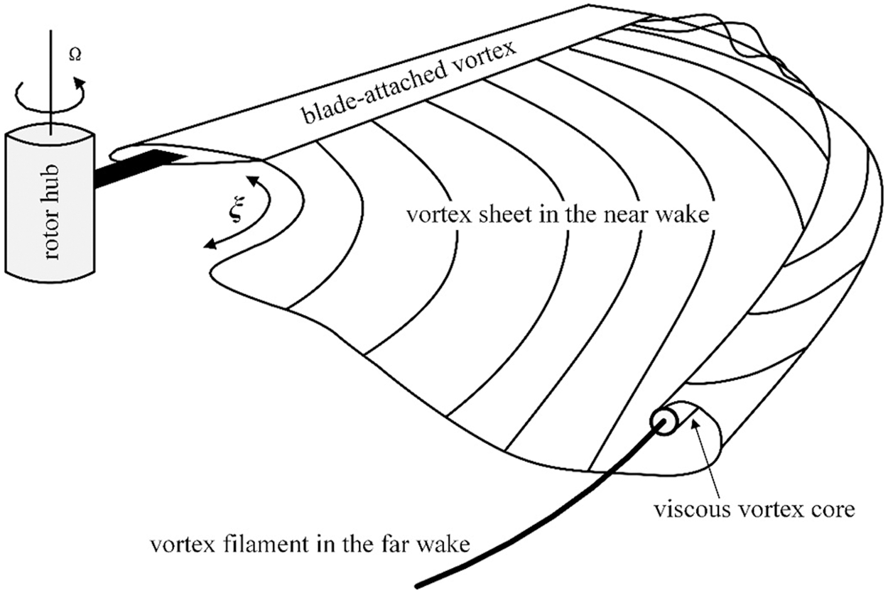
Figure 1: Sketch of the rotor wake formation

In Formula (1), the u∞ and ufwbb are correlated to the helicopter flight status, including the rotor blade motion. These can be determined through the trim calculation of the following helicopter flight dynamics model. Fig. 2 shows a sample of the convergent rotor wake of the UH-60A helicopter in hover.

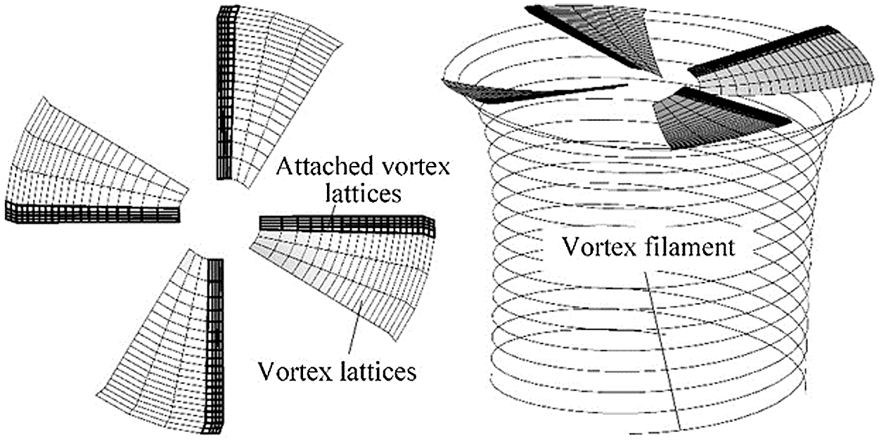
Figure 2: Sketch of the rotor wake description ( Nr=20 , Nc=4 , Nw=3 , Nfw=144 )

2.2 Rotor Icing Model

Considering the rotor icing, an engineering rotor icing model needs to be developed. This mainly involves the introduction of the icing-related increments of rotor thrust, horizontal force, side force, torque coefficients, and icing-related increment of flapping coefficients into the uniced flight dynamics model.

The basic lift and drag coefficients of the rotor-blade airfoil due to icing are, as follows:

{C′l=(1+ΔCl/Cl)ClC′d=(1+ΔCd/Cd)Cd (2)

The coefficients for rotor thrust, side force, horizontal force, and torque due to icing are, as follows:

{C′T=CT+ΔCTC′Y=CY+ΔCYC′H=CH+ΔCHC′Q=CQ+ΔCQ (3)

The iced-rotor flapping model in the Fourier series form can be presented, as follows:

{a′0=a0+Δa0a′1c=a1c+Δa1ca′1s=a1s+Δa1s (4)

In Formulas (2), (3), and (4), the rotor thrust, horizontal force, side force and torque coefficients, as well as the rotor flapping coefficients, were calculated using the following Rotor Discrete Aerodynamic Model. Furthermore, the corresponding increments caused by icing can be calculated by the established engineering icing model in [7] and [8].

2.3 Rotor Discrete Aerodynamics Model

The rotor discrete aerodynamic model was developed to embed the rotor free-vortex wake model and rotor icing model into the following helicopter flight dynamics model. In the process of modeling and numerical simulation, based on the principle of equal annular area, the rotor disc was divided into Nr×Nψ calculating sectors, with Nr radial stations for each of the Nψ azimuthal sectors, as shown in Fig. 3.

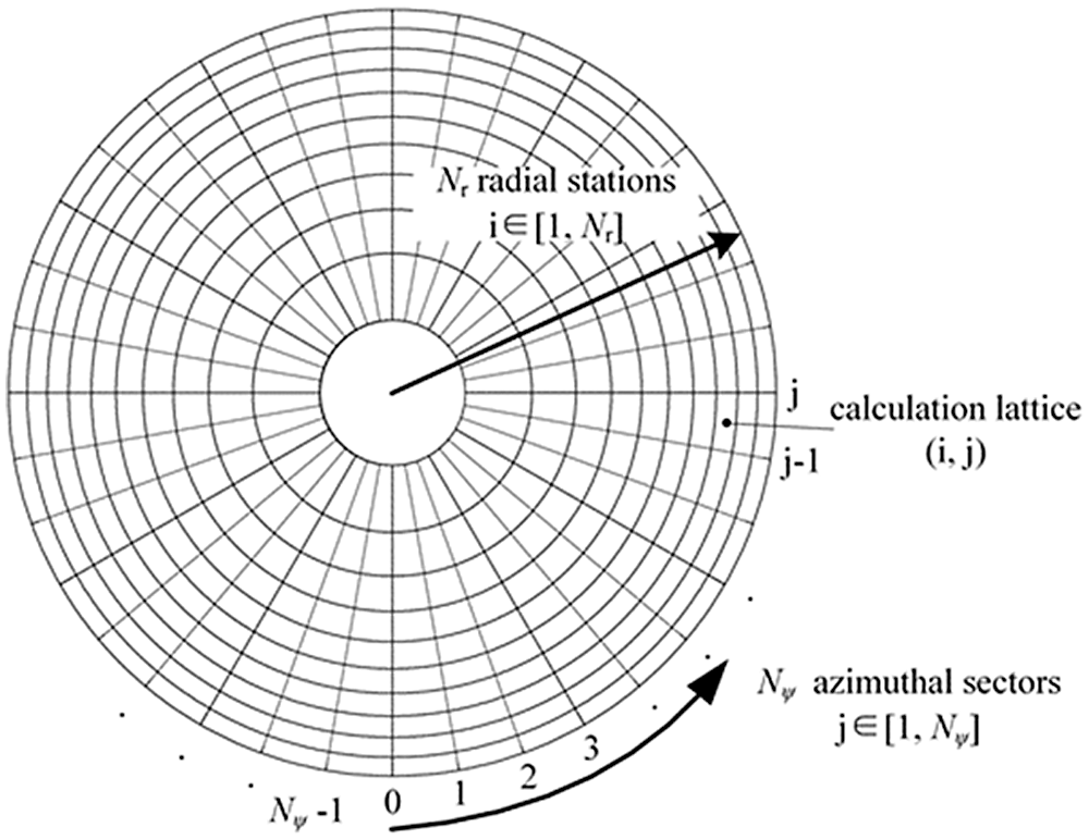
Figure 3: Sketch of the rotor disc discretization ( Nr=10 , Nψ=36 )

The discrete expressions of the rotor thrust, horizontal force, side-force, and torque coefficients can be deduced, as follows:

(CTCHCYCQ)=σΔψ4π∑i=1Nr∑j=1Nψ(Fc(i,j)cos⁡β(j)Fs(i,j)sin⁡ψ(j)−Fc(i,j)sin⁡β(j)cos⁡ψ(j)−Fs(i,j)cos⁡ψ(j)−Fc(i,j)sin⁡β(j)sin⁡ψ(j)−Fs(i,j)(r¯(i)cos⁡β(j)+e¯)) (5)

where,

Fc(i,j)=(Cl(i,j)cos⁡β∗(i,j)−Cd(i,j)sin⁡β∗(i,j))F0(i,j) (6)

Fs(i,j)=(Cl(i,j)sin⁡β∗(i,j)+Cd(i,j)cos⁡β∗(i,j))F0(i,j) (7)

F0(i,j)=[(u¯T(i,j))2+(u¯P(i,j))2]Δr¯(i) (8)

The Cl(i,j) and Cd(i,j) in icing conditions can be derived from the above rotor icing model, that is, by using Formula (2).

The equations for the rotor coning and first-order longitudinal and lateral flapping coefficients in the rotor flapping model are, as follows:

{f1(a0,a1c,a1s)=IbΩ2a0−MT0+Msg=0f2(a0,a1c,a1s)=MTc+2PRΩIb=0f3(a0,a1c,a1s)=MTs−2QRΩIb=0 (9)

The expressions of MT0 , MTc and MTs are, as follows:

MT0=Δψ4πρc(ΩR)2R2∑i=1Nr⁡∑j=1Nψ⁡Fc(i,j)r¯(i) (10)

MTc=Δψ2πρc(ΩR)2R2∑i=1Nr⁡∑j=1Nψ⁡Fc(i,j)r¯(i)cos⁡ψ(j) (11)

MTs=Δψ2πρc(ΩR)2R2∑i=1Nr⁡∑j=1Nψ⁡Fc(i,j)r¯(i)sin⁡ψ(j) (12)

When Formula (5) was solved, the rotor coning and first-order longitudinal and lateral flapping coefficients can be obtained by solving the nonlinear equations, that is, Formula (9).

2.4 Helicopter Flight Dynamics Model

In the present study, a nonlinear flight dynamic model of a single rotor helicopter with a tail rotor was developed, as follows:

{mGV˙B+mGωB×VB=FBH˙B+ωB×HB=MBωB=TEuler[θ˙B,ϕ˙B,ψ˙B]T (13)

In Formula (13), the resultant force vector ( FB ) and resultant moment vector ( MB ) that acts on the helicopter can be presented, as follows:

{FB=FR+FTR+FFUS+FHT+FVT+FGMB=MR+MTR+MFUS+MHT+MVT (14)

In the above formula, the rotor force ( FR ) and moment ( MR ) vectors that act on the helicopter are the functions of rotor thrust, horizontal force, side-force and torque coefficients in the above rotor discrete aerodynamic model.

{FR=f1(CT,CH,CY,CQ)MR=f2(CT,CH,CY,CQ) (15)

In Formula (14), the tail rotor force ( FTR ) and force moment ( MTR ) vectors can be calculated using the traditional Rotor Momentum Theory [31]. The force and force moment vectors of fuselage ( FFUS , MFUS ), horizontal tail ( FHT , MHT ), and vertical tail ( FVT , MVT ) can be obtained using the wind tunnel test data [32].

3  Implementation Procedure

In the present study, the rotor free-vortex wake model and rotor icing model were incorporated into the rotor discrete aerodynamics model to output the FR′ and MR′ needed in the flight dynamics model. By trimming the flight dynamics model, the numerical simulation of the helicopter rotor free-vortex wake in icing conditions could be conducted.

As shown in Fig. 4, the initial uniced helicopter flight dynamics trim calculation can be conducted using the Rotor Vortex Model (RVM) [33]. Then, the rotor free-vortex wake iteration can be conducted to solve the convergent wake geometry. In addition, the non-uniform distribution of the rotor-induced velocity and rotor flapping coefficients can be obtained using the proposed Cross-Coupling-Iteration (CCI) algorithm. Subsequently, the rotor icing model predicts the increments of the iced rotor force and torque, as well as the rotor flapping coefficients caused by icing. Then, the calculation of the rotor discrete aerodynamics model can be conducted. When the trim calculation of the helicopter flight dynamics model becomes convergent, the numerical simulation of the helicopter rotor wake in icing conditions is completed. Otherwise, the rotor free-vortex wake iteration should be conducted again based on the present trim state.

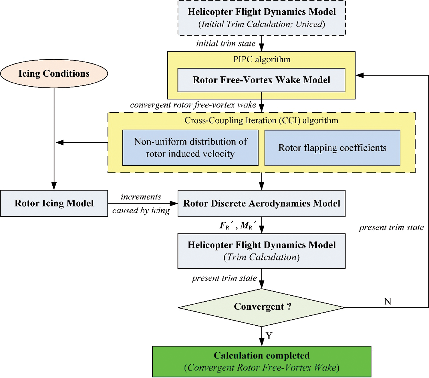
Figure 4: Flowchart for the numerical simulation

4  Numerical Method

4.1 PIPC Algorithm

Bagai and Leishman’s PIPC algorithm [21] was adopted to solve the above governing equation in Formula (1). Fig. 5 presents the solution domain, solution direction, grid setting, periodic boundary conditions, etc. For the numerical solution of the far wake in finite space, the far wake can be truncated using the concept of the boundary wake [34].

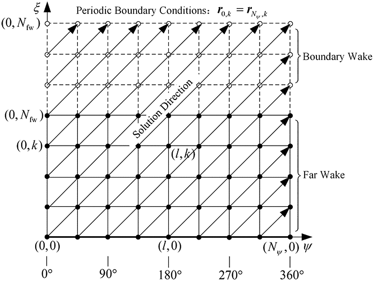
Figure 5: Sketch of the solution domain and solution direction

Using the five-point central difference method, the first order differential terms of the governing equation in Formula (1) can be presented, as follows:

{∂r∂ψ|(l+1/2,k+1/2)=12(rl,k+1−rl,kΔψ+rl+1,k+1−rl+1,kΔψ)∂r∂ξ|(l+1/2,k+1/2)=12(rl+1,k−rl,kΔξ+rl+1,k+1−rl,k+1Δξ) (16)

The Δξ is equal to Δψ for the convenience of the numerical solution. The velocity term ( V ) of the governing equation in Formula (1) can be deduced as the mean velocity.

V(rl+1/2,k+1/2)=[V(rl,k)+V(rl,k+1)+V(rl+1,k+1)+V(rl+1,k)]/4 (17)

Then, the governing equation in Formula (1) can be presented, as follows:

rl+1,k+1=rl,k+Δψ4Ω[V(rl,k)+V(rl,k+1)+V(rl+1,k+1)+V(rl+1,k)] (18)

Since both the five-point central difference and mean velocity approximation have second-order accuracy, the above Formula (18) also has second-order accuracy for the governing equation in Formula (1). Based on the Formula (18), the governing equation can be solved through the calculation of the prediction and correction in each iteration using Bagai and Leishman’s PIPC algorithm.

4.2 Cross Coupling Iteration (CCI) Algorithm

In the present study, the Cross-Coupling-Iteration (CCI) algorithm was proposed to calculate the non-uniform distribution of rotor-induced velocity and the corresponding flapping coefficients (Fig. 6) for avoiding computational divergence.

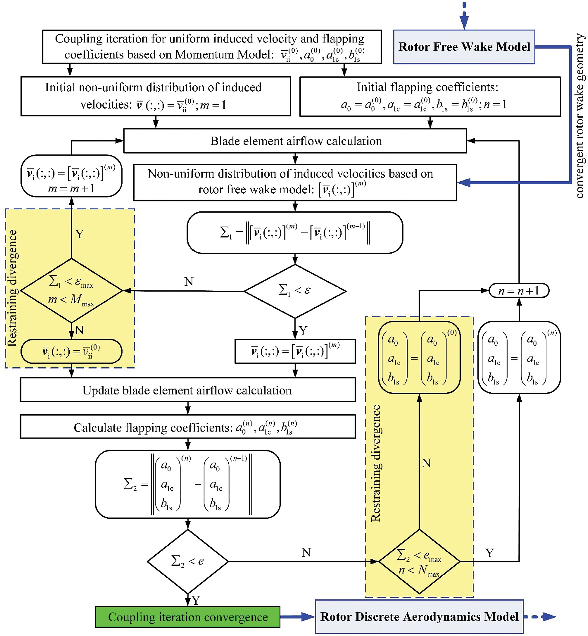
Figure 6: Flow chart for the CCI method

In the CCI algorithm, two constraints were performed: the constraint on rotor-induced velocity iteration, and the constraint on rotor flapping coefficients iteration. When the non-uniform distribution of rotor-induced velocity iteration approaches to the divergence, the uniform distribution of rotor-induced velocity, based on the Rotor Momentum Model (RMM) [33], can be used to as the iteration values at the moment, in order to enter the next iteration. If the rotor flapping coefficients iteration is not convergent, the rotor flapping coefficients, based on the RMM, can be used to as the iteration values at the moment, in order to enter the next iteration.

4.3 Verification of the Numerical Calculation Method

The validity and accuracy of the numerical calculation method was verified through comparison with the available experimental measurements [34]. The model rotor geometry and operating conditions for the rotor configuration is summarized in Tab. 1.

Table 1: Operating conditions for the rotor configuration

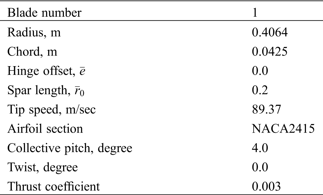
Fig. 7 presents the free-vortex wake predictions along with the experimental measurements. This indicates that the predictions and experimental measurements are in good agreement, except for some discrepancies in the wake age, which ranged from 0 to 180° (i.e., the first circle of the rotor wake). The reason for these discrepancies is that the release point (Fig. 7) of the blade tip vortex in the model is located on the quadrilateral vortex lattice of the near wake, while the near wake is fixed in the tangent plane of the trailing edge of blade mid-arc surface. Hence, the vortex sheet of the near wake occupies a fixed space along with the vertical down direction, allowing the rotor free-vortex wake of the first circle to have a larger change, when compared to the experimental measurements. However, according to the results after the first circle of the rotor wake, the near wake setting method (i.e., fixed in the tangent plane of the trailing edge of the blade mid-arc surface) does not affect the calculation accuracy of the subsequent rotor free-vortex wake.

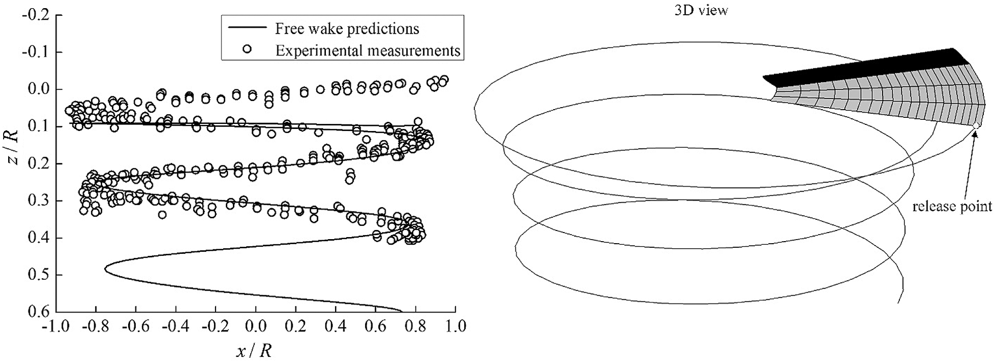
Figure 7: Free-vortex wake predictions along with the experimental measurements

Fig. 8 shows the convergent rotor wake geometries of the UH-60A helicopter in hovering, and at different forward flight velocities in clean ice conditions. This shows that the free-vortex wake method embedded in the helicopter flight dynamics model can well-capture the rotor wake geometric characteristics. Especially, with the increase of forward flight velocity, the process of the tip vortex rolling up of the rotor blade is well-demonstrated.

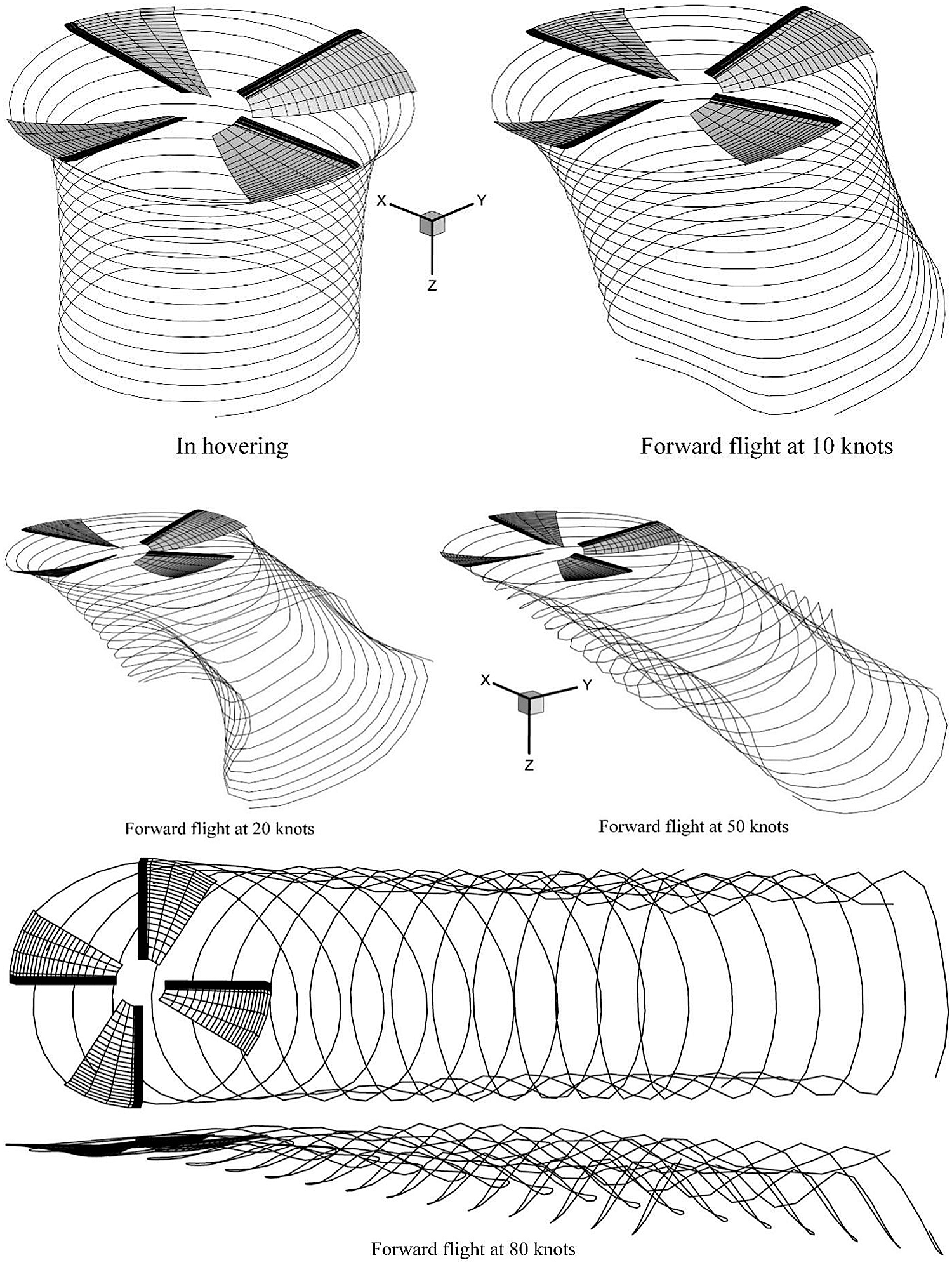
Figure 8: The rotor free-vortex wake geometries of the UH-60A helicopter at different flight velocities

5  Results and Analysis

The effects of icing on the rotor-vortex wake due to icing time and atmospheric temperature were mainly analyzed using the above mathematical model and the corresponding procedure, as well as the numerical method. Merely the wake of one blade at the azimuth of zero degree was depicted and analyzed in detail for convenience. The basic icing conditions are presented in Tab. 2.

Table 2: Basic icing conditions

5.1 Icing Time

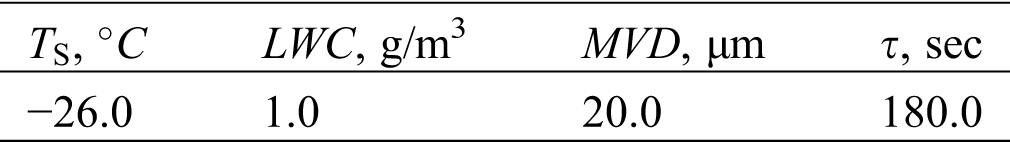
Fig. 9 presents the effects of icing on the rotor free-vortex wake due to icing time in hovering. In Fig. 9, the rotor icing makes the wake geometry slightly sink. This also induces the wake geometry to slightly move along the azimuth of 180 and 90 degrees. Furthermore, as the icing time increases, the variation trend become increasingly obvious. Furthermore, Fig. 9 presents the heights of the blade tip vortex filament versus vortex age angle, and the specific changes in the sunk amplitude of the free-vortex wake.

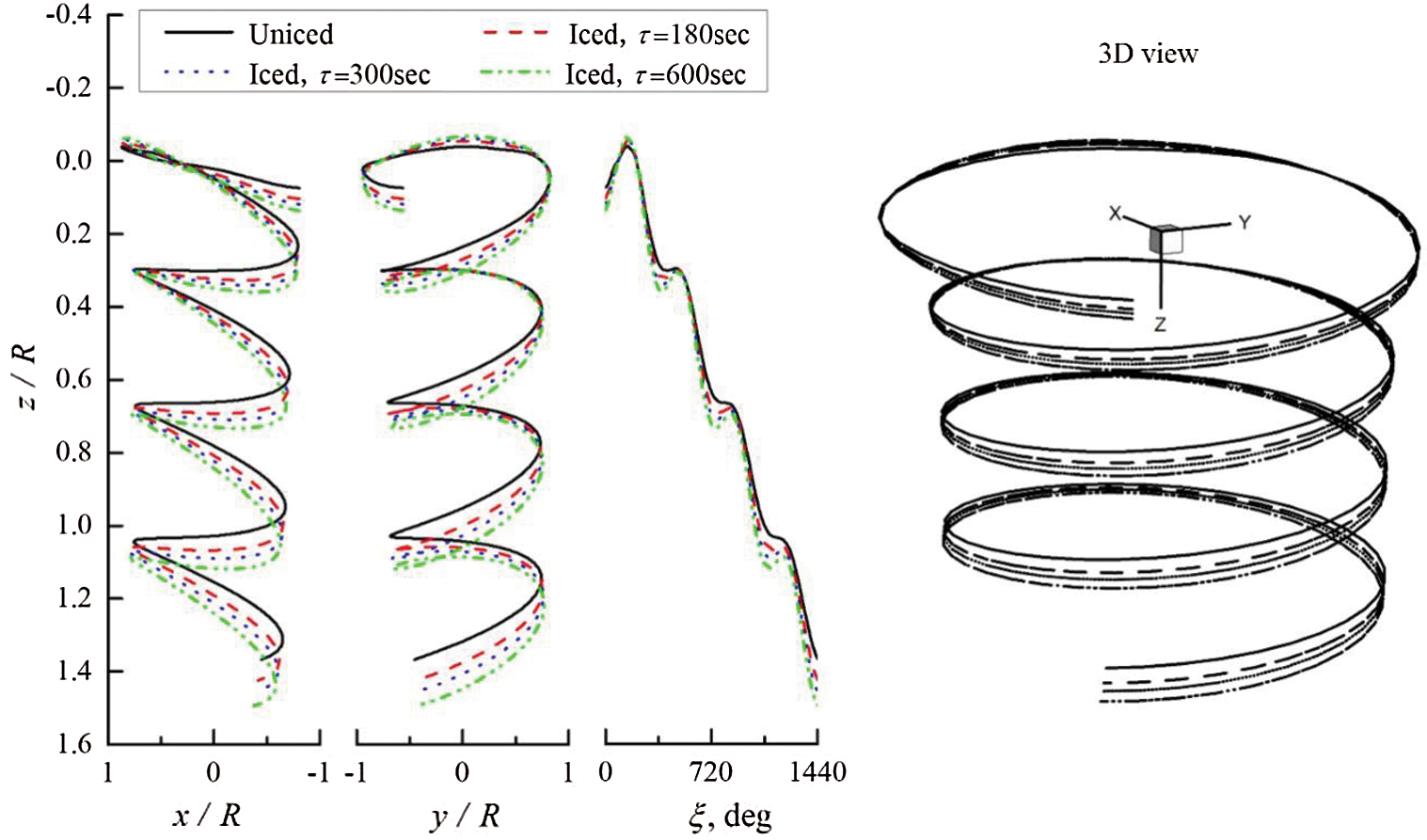
Figure 9: Effects of icing on the rotor free-vortex wake due to τ in hovering

Some of the reasons for the rotor free-vortex wake changes with icing time might be due to the effects of icing on the angle of attack (AOA) of the rotor blade. In comparing the uniced distribution of AOA, Fig. 10 presents the effects of icing on the distribution of AOA due to the icing time, which ranged from 180 s to 300 s, and to 360 s. This indicates that the AOA of the rotor blade increases with the icing time. Furthermore, at the blade tip area in the front half part, and at the blade root area in the back half part of the rotor disc, the AOA of the rotor blade exhibits an evident increase with icing time. The reason for the icing effects on the AOA of the rotor blade might be due to the rotor performance degradation. In this situation, the inflight helicopter needs to maintain a stable hover by at least increasing the collective pitch control, in order for the AOA to increases.

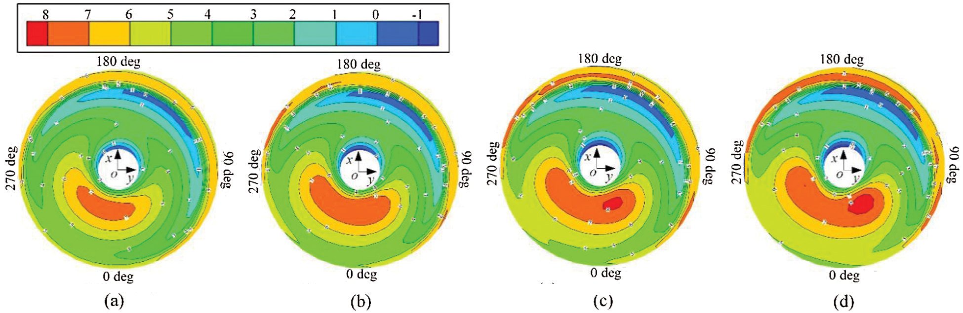
Figure 10: Effects of icing on the AOA of the rotor blade due to τ in hovering. (a) Uniced, (b) Iced, τ = 180 s, (c) Iced, τ = 300 s, (d), Iced, τ = 360 s

5.2 Atmospheric Temperature

Fig. 11 presents the effects of icing on the rotor free-vortex wake due to atmospheric temperature in hovering. As shown in Fig. 11, the rotor icing induced the free-vortex wake to slightly sink when the atmospheric temperature degraded from −12°C to −20°C. However, this caused the sunk trend to slightly recover when the atmospheric temperature continued to degrade from −20°C to −26°C. Fig. 11 presents the heights of the blade tip vortex filament versus vortex age angle, and the specific changes in amplitude of this trend.

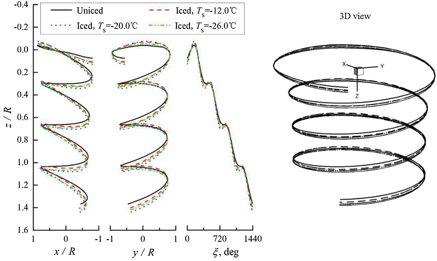
Figure 11: Effects of icing on rotor wake due to TS in hovering

Some of the reasons for this change trend might be due to the temperature effects. In general, the performance penalties caused by glaze ice is more serious than mixed ice, and subsequently by rime ice. The rotor icing tunnel test data indicated that as the temperature increased, the accreted ice shape on the outer portion of the rotor blades changed from rime to mixed, and subsequently to glaze, increasing the performance penalties [35]. In this section, with the use of the ice shape definition method [8], the distribution of the ice shape on the rotor disc at different atmospheric temperatures was calculated to validate the change trend of the effects of icing on the rotor free-vortex wake due to atmospheric temperature, as shown in Fig. 12.

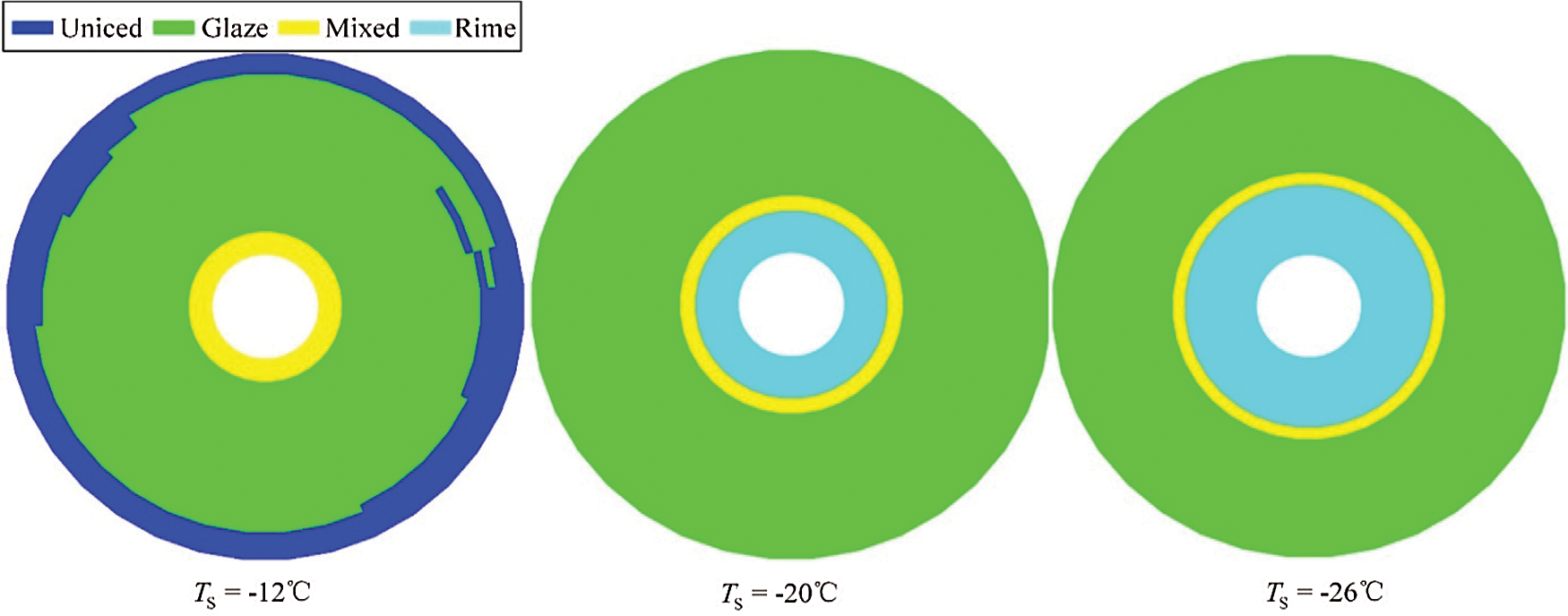
Figure 12: The distribution of the ice shape on the blades of the rotor disc in hovering

Fig. 12 shows that the range of the glaze ice that accreted on the outer portion of the rotor blades significantly increased when the atmospheric temperature degraded from −12°C to −20°C, increasing the performance penalties, and subsequently making the rotor downstream wake sink (Fig. 11). However, the range of the rime ice that accreted on the inner portion of the rotor blades evidently increased when the atmospheric temperature degrades from −20°C to −26°C, decreasing the performance penalties and making the rotor downstream free-vortex wake have a slightly reverted change trend to the uniced state (Fig. 11). The reason for this is that the performance penalties due to rime ice is lower than the glaze ice, and that this has an irregular shape. In addition, the uniced area on the blade tip region in Fig. 12 was generated by an extremely high local temperature, preventing the occurrence of ice accretion. The reason for this is that there might be a positive correlation between the high local temperature and the high local Mach number at the blade tip region.

5.3 Forward Flight Velocity

For further comparison with the situation of the high local temperature at the blade tip region at hover in Fig. 11, Fig. 13 presents the distribution of the ice shape on the blades of the rotor disc at a forward flight of 60 knots, with TS=−12∘C , τ=60s and LWC=0.75g/m3 . Compared with Fig. 12, when a helicopter changes from hover to forward flight, the icing area might gradually diffuses to the blade tip at the retreating blade region (left side direction of Figs. 12 and 13) due to the local temperature reduction on the retreating blade region, and the reduction in the local Mach number of the blade tip region at forward flight velocity.

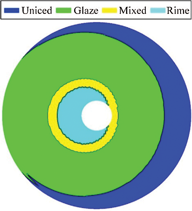
Figure 13: The distribution of the ice shape on the blades of the rotor disc at a forward flight of 60 knots

Fig. 14 presents the comparison of the lift-to-drag ratio distribution of the rotor disc before and after icing at a forward flight of 60 knots. This evidently indicates that the lift-to-drag ratio evidently drops when the helicopter rotor encounters ice accretion at forward flight velocity.

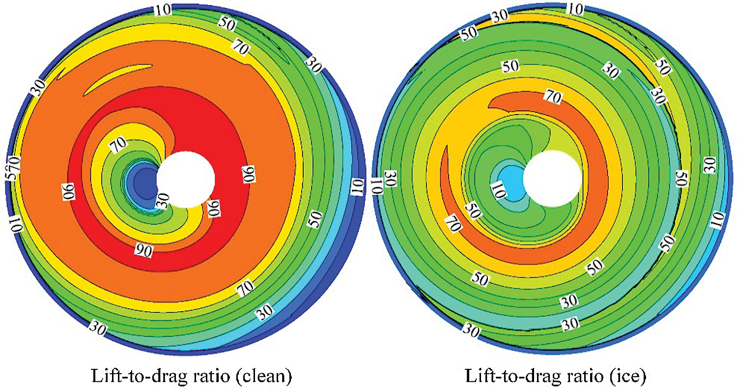
Figure 14: The lift-to-drag ratio distribution of the rotor disc at a forward flight of 60 knots

6  Summary

By incorporating the rotor free-vortex wake model and rotor icing model into the rotor discrete aerodynamics model, and using the proposed Cross Coupling Iteration (CCI) algorithm, the trim calculation of the helicopter flight dynamics model in icing conditions was conducted, in order to acquire the convergent rotor free-vortex wake geometry, and investigate the effects of icing on the rotor free-vortex wake. The following conclusions that might have some significance in helicopter flight safety encounters with ice accretion can be mainly summarized, as follows:

1.   The proposed numerical simulation method appears to be an adequate tool for helicopter rotor free-vortex wake analysis in icing conditions.

2.   Both the sunk trend of the rotor free-vortex wake due to icing and the variation of the ice shape on the rotor blades might lead to rotor aerodynamic degradation: on one hand, ice accretion causes the rotor free-vortex wake to sink, and this sinking trend becomes more evident with the increase in icing time. On the other hand, a rime-ice shape initially occurs on the inner portion of rotor blades, and diffuses outward along the blade with the decrease in atmospheric temperature. In addition, the uniced area of the rotor blade tip is generated by the extremely high local temperature, preventing the occurrence of ice accretion. However, a glaze-ice shape occurs when the atmospheric temperature continues to decrease.

3.   As shown in the forward flight velocity analysis, the lift-to-drag ratio would evidently drop when helicopter rotor encounters ice accretion. When the helicopter changes from hover to forward flight in the typical condition of TS=−12∘C , the glaze ice might gradually diffuses to the blade tip on the retreating blade region, which is due to the decrease in local temperature on the retreating blade region, and the reduction in local Mach number at the blade tip region at forward flight. This phenomenon might provide a great enlightenment for the design of anti-icing and deicing of helicopter rotor blades.

Funding Statement: The author(s) received no specific funding for this study.

Conflicts of Interest: The authors declare that they have no conflicts of interest to report regarding the present study.

References

 1.  Lewis, R. B. (1974). U. S. army helicopter icing qualification program. AIAA 6th Aircraft Design, Flight Test and Operations Meeting, Los Angeles, USA. [Google Scholar]

 2.  Korkan, K., Dadone, L., Shaw, R. (1984). Helicopter rotor performance degradation in natural icing encounter. Journal of Aircraft, 21(1), 84–85. DOI 10.2514/3.48226. [Google Scholar] [CrossRef]

 3.  Britton, R. K. (1992). Development of an analytical method to predict helicopter main rotor performance in icing condition. 30th Aerospace Sciences Meeting and Exhibit, Reno, NV, USA. DOI 10.2514/6.1992-418. [Google Scholar] [CrossRef]

 4.  Marques, S., Badcock, K. J., Gooden, J. H. M., Gates, S., Maybury, W. (2010). Validation study for prediction of iced aerofoil aerodynamics. Aeronautical Journal, 114(1152), 103–111. DOI 10.1017/S0001924000003572. [Google Scholar] [CrossRef]

 5.  Kelly, D., Habashi, W. G., Quaranta, G., Masarati, P., Fossati, M. (2018). Ice accretion effects on helicopter rotor performance, via multibody and CFD approaches. Journal of Aircraft, 55(3), 1165–1176. DOI 10.2514/1.C033962. [Google Scholar] [CrossRef]

 6.  Chen, X., Zhao, Q., Barakos, G. (2019). Numerical analysis of aerodynamics of iced rotor in forward flight. AIAA Journal, 57(1), 1–13. DOI 10.2514/1.J058146. [Google Scholar] [CrossRef]

 7.  Cao, Y. H., Li, G. Z., Zhong, G. (2010). Tandem helicopter trim and flight characteristics in the icing condition. Journal of Aircraft, 47(5), 1559–1569. DOI 10.2514/1.C000183. [Google Scholar] [CrossRef]

 8.  Cao, Y. H., Li, G. Z., Hess, R. (2012). Helicopter flight characteristics in icing conditions. The Aeronautical Journal, 116(1183), 963–979. DOI 10.1017/S0001924000007375. [Google Scholar] [CrossRef]

 9.  Fortin, G., Perron, J. (2009). Spinning rotor blade tests in icing wind tunnel. 1st AIAA Atmospheric and Space Environments Conference, San Antonio, Texas, USA. DOI 10.2514/6.2009-4260. [Google Scholar] [CrossRef]

10. Brunetti, M., Chatterton, S., Toscani, N., Mauri, M., Carmeli, M. S. et al. (2020). Wireless power transfer with temperature monitoring interface for helicopter rotor blade ice protection. 2020 AIAA/IEEE Electric Aircraft Technologies Symposium, USA. [Google Scholar]

11. Rosa, F. D., Esposito, A. (2012). Electrically heated composite leading edges for aircraft anti-icing applications. Fluid Dynamics & Materials Processing, 8(1), 107–128. [Google Scholar]

12. Xin, M., Zhong, G., Cao, Y. H. (2020). Numerical simulation of an airfoil electrothermal-deicing-system in the framework of a coupled moving-boundary method. Fluid Dynamics & Materials Processing, 16(6), 1063–1092. DOI 10.32604/fdmp.2020.013378. [Google Scholar] [CrossRef]

13. Cao, Y. H., Chen, K. (2010). Helicopter icing. Aeronautical Journal, 114(1152), 83–90. DOI 10.1017/S0001924000003559. [Google Scholar] [CrossRef]

14. Cao, Y. H., Wu, Z., Su, Y., Xu, Z. (2015). Aircraft flight characteristics in icing conditions. Progress in Aerospace Sciences, 74(1152), 62–80. DOI 10.1016/j.paerosci.2014.12.001. [Google Scholar] [CrossRef]

15. Cao, Y. H., Tan, W. Y., Wu, Z. L. (2018). Aircraft icing: an ongoing threat to aviation safety. Aerospace Science and Technology, 75(5), 353–385. DOI 10.1016/j.ast.2017.12.028. [Google Scholar] [CrossRef]

16. Cao, Y. H., Xin, M. (2020). Numerical simulation of supercooled large droplet icing phenomenon: A review. Archives of Computational Methods in Engineering, 27(4), 1231–1265. DOI 10.1007/s11831-019-09349-5. [Google Scholar] [CrossRef]

17. Wu, W. M., Zhou, C. D. (2020). A numerical study of the tip wake of a wind turbine impeller using extended proper orthogonal decomposition. Fluid Dynamics & Materials Processing, 16(5), 883–901. DOI 10.32604/fdmp.2020.010407. [Google Scholar] [CrossRef]

18. Gupta, S., Leishman, J. G. (2005). Accuracy of the induced velocity from helicoidal wake vortices using straight-line segmentation. AIAA Journal, 43(1), 29–40. DOI 10.2514/1.1213. [Google Scholar] [CrossRef]

19. Beyer, F., Matha, D., Sebastian, T., Lackner, M. A. (2012). Development, validation and application of a curved vortex filament model for free vortex wake analysis of floating offshore wind turbines. 50th AIAA Aerospace Sciences Meeting including the New Horizons Forum and Aerospace Exposition, Nashville, Tennessee, USA. DOI 10.2514/6.2012-371. [Google Scholar] [CrossRef]

20. Premaratne, P., Hu, H. (2017). A novel vortex method to investigate wind turbine near-wake characteristics. 35th AIAA Applied Aerodynamics Conference, Colorado, USA. [Google Scholar]

21. Bagai, A., Leishman, J. (1995). Rotor free-wake modeling using a pseudo-implicit technique–including comparisons with experimental Data. Journal of the American Helicopter Society, 40(3), 29–41. DOI 10.4050/JAHS.40.29. [Google Scholar] [CrossRef]

22. Lee, J., Yee, K. (2016). Improvement of computational efficiency for rotor flowfield analysis using computational-fluid-dynamics-free-wake coupling method. Journal of Aircraft, 53(6), 1953–1958. DOI 10.2514/1.C033894. [Google Scholar] [CrossRef]

23. Cao, Y. H., Lv, S. J., Li, G. Z. (2014). A coupled free-wake/panel method for rotor/fuselage/empennage aerodynamic interaction and helicopter trims. Proceedings of the Institution of Mechanical Engineers, Part G: Journal of Aerospace Engineering, 229(3), 435–444. DOI 10.1177/0954410014534203. [Google Scholar] [CrossRef]

24. Halder, A., Benedict, M. (2019). Free-wake based nonlinear aeroelastic modeling of UAV scale cycloidal rotor. AIAA Aviation 2019 Forum, Dallas, TX, USA. [Google Scholar]

25. Spoldi, S., Ruckel, P. (2003). High fidelity helicopter simulation using free wake, lifting line tail, and blade element tail rotor models. 59th Annual Forum of AHS, Phoenix AZ, USA. [Google Scholar]

26. Horn, J., Bridges, D., Wachspress, D. (2005). Implementation of a free vortex wake model in real time simulation of rotorcraft. 61th Annual Forum of AHS, Grapevine TX, USA. [Google Scholar]

27. Wachspress, D., Quackenbush, T., Boschitsch, A. (2003). First-principles free vortex wake analysis for helicopter and tilt-rotors. 59th Annual Forum of AHS, Phoenix AZ, USA. [Google Scholar]

28. Ribera, M. (2007). Helicopter flight dynamics simulation with a time accurate free vortex wake model. University of Maryland, USA. [Google Scholar]

29. Omri, R., Vladimir, K. (2018). Free-wake-based dynamic inflow model for hover, forward, and maneuvering flight. Journal of the American Helicopter Society, 63(1), 1–16. [Google Scholar]

30. Katz, J., Plotkin, A. (2001). Low-speed aerodynamics. UK: Cambridge University Press. [Google Scholar]

31. Cao, Y. H., Li, G. Z., Yang, Q. (2009). Studies of trims, stability, controllability, and some flying qualities of a tandem rotor helicopter. Proceedings of the Institution of Mechanical Engineers. Part G: Journal of Aerospace Engineering, 223(2), 171–177. [Google Scholar]

32. Howlett, J. J. (1981). UH-60A black hawk engineering simulation program: Volume I–Mathematical model. NASA CR 166309. Washington DC, USA. [Google Scholar]

33. Cao, Y. H. (2009). Principles of helicopter flight dynamics. Oxfordshire, UK: Coxmoor Publishing Company. [Google Scholar]

34. Bhagwat, M. (2001). Mathematical modeling of the transient dynamics of helicopter rotor wakes using a time accurate free vortex methods. MD, USA: University of Maryland. [Google Scholar]

35. Flemming, R., Randall, K., Thomas, H. (1994). Role of wind tunnels and computer codes in the certification and qualification of rotorcraft for flight in forecast icing. NASA TM-106747, Washington DC, USA. [Google Scholar]

This work is licensed under a Creative Commons Attribution 4.0 International License, which permits unrestricted use, distribution, and reproduction in any medium, provided the original work is properly cited.