Materials Processing
| Fluid Dynamics & Materials Processing |
DOI: 10.32604/fdmp.2021.010925
ARTICLE
Fluid-Structure Interaction in Problems of Patient Specific Transcatheter Aortic Valve Implantation with and Without Paravalvular Leakage Complication
1Department of Aerospace Engineering, Universiti Putra Malaysia, Serdang, 43400, Malaysia
2Department of Aeronautical and Automobile Engineering, Manipal Institute of Technology, Manipal Academy of Higher Education, Manipal, 576104, India
3Department of Medicine, Universiti Putra Malaysia, Serdang, 43400, Malaysia
4Department of Biological Function and Engineering, Kyushu Institute of Technology, Kitakyushu, Japan
5Fakulti Kejuruteraan Mekanikal, Universiti Teknikal Malaysia Melaka, Hang Tuah Jaya, 76100, Malaysia
6Aerospace Malaysia Research Center, Universiti Putra Malaysia, Serdang, 43400, Malaysia
*Corresponding Author: Adi Azriff Basri. Email: adiazriff@upm.edu.my
Received: 07 April 2020; Accepted: 29 January 2021
Abstract: Paravalvular Leakage (PVL) has been recognized as one of the most dangerous complications in relation to Transcathether Aortic Valve Implantation (TAVI) activities. However, data available in the literature about Fluid Structure Interaction (FSI) for this specific problem are relatively limited. In the present study, the fluid and structure responses of the hemodynamics along the patient aorta model and the aortic wall deformation are studied with the aid of numerical simulation taking into account PVL and 100% TAVI valve opening. In particular, the aorta without valve (AWoV) is assumed as the normal condition, whereas an aorta with TAVI 26 mm for 100% Geometrical Orifice Area (GOA) is considered as the patient aorta with PVL complication. A 3D patient-specific aorta model is elaborated using the MIMICS software. Implantation of the identical TAVI valve of Edward SAPIEN XT 26 (Edwards Lifes ciences, Irvine, California) is considered. An undersized 26 mm TAVI valve with 100% valve opening is selected to mimic the presence of PVL at the aortic annulus. The present research indicates that the existence of PVL can increase the blood velocity, pressure drop and WSS in comparison to normal conditions, thereby paving the way to the development of recirculation flow, thrombus formation, aorta wall collapse, aortic rupture and damage of endothelium.
Keywords: Paravalvular Leakage (PVL); hemodynamics; transcatheter aortic valve implantation (TAVI); fluid-structure interaction (FSI); edward sapien valve aortic valve (ESV); aortic stenosis (AS)
Transcatheter Aortic Valve Implantation (TAVI) is the current emerging solution for high-risk patients with severe symptoms of Aortic Stenosis (AS). It is recognized as the minimally invasive heart valve replacement in patients with high surgical risk and multi-morbidity [1,2]. TAVI has received great attention from broad research studies and clinical experiences due to the lower operative risk with shorter time of recovery compared to surgical aortic valve (SAV) replacement. However, one of the serious complications which received tremendous attention from many researchers worldwide after undergone TAVI is the Paravalvular Leakage (PVL) [3–5]. PVL is referred to as a small opening between the prosthetic valve and aortic annulus, where the blood flowed through the uncovered portion of the stent frame [6]. The under-expansion of the prosthetic valve, undersizing, interfering on stent expansion due to the impingement of calcium nodules and mal-positioning of the valve lead to the cause of this PVL complication [6,7]. PVL can be graded as mild, moderate and severe with (7.8–40.8%), (5–36.9%) and (0.5–13.6%), respectively where PVL remains a frequent issue after implantation [8].
With the emerging technology, the coupling technique of clinical imaging with numerical simulation provides better tools for researchers around the world to understand in detail the impact of stenosis development in patients’ health especially on the hemodynamics behavior [9–18]. Besides that, this technology also has inspired a lot of researchers to study the blood flow behavior in cardiovascular diseases such as renal artery stenosis, aortic aneurysm, aortic dissection, and etc [19–27].
Nowadays, the growing technology of simulation has produced a superior coupling technique between Finite Element Analysis (FEA) and Computational Fluid Dynamics (CFD) method which is known as Fluid-Structure Interaction (FSI) analysis. This technique has the capability of mimicking the realistic model of human organs where the responses between fluid flow and structural behavior can be simulated using this novel FSI technique. Several research studies available related to TAVI using the novel technique of the FSI approach.
Auricchio et al. [28] demonstrated the effect of stent crimping and deployment of Edwards SAPIEN implantation within aortic root geometries using FEA. Meanwhile, another study by Bianchi et al. [29] investigated the effect of various TAVI deployment locations on the risk of valve migration. Bianchi et. al [30] in another study performed both FEA and CFD analyses separately to analyze the influence of procedural parameters on post-deployment. The authors investigated the hemodynamics of three retrospective clinical cases related to PVL. The research only focused on the degree of PVL located at the aortic annulus where the results showed the right positioning and balloon over-expansion may impact the PVL volume reduction as high as 47%.
On the other hand, Rocatello et al. [31] proposed a new framework to optimize the TAVI valve design using FEA and CFD analyses. The effect of two geometrical parameters of the frame, height of the first row cells and diameter at inflow ventricular were investigated and the device performance was compared within the 12 patients. The results suggested that better apposition of the devices to the aortic root may prevent aortic regurgitation. Roccatello et al. [32] further the study by investigating the influence of Lotus size/position related to paravalvular aortic regurgitation (AR) using FEA and CFD analysis. The results showed a large valve size and not in position produced higher contact pressure and reduced the predicted AR.
Related to FSI simulation, Mao et al. [33] compared both analyses of FEA and FSI of the TAVI model to investigate the stress and strain distribution effects on TAVI leaflets. The results proved that the FSI model produced 13–18% higher stress than the FEA model. On the other hand, Luraghi et al. [34] have developed a robust framework to perform patient-specific FSI simulation of TAVI with PVL complications. The results showed the mild and moderate PVL produced coherent values of effective regurgitant orifice area and regurgitant volume. However, no research available on the investigation of the effects of PVL through the aorta. Due to this matter, the investigation of PVL complications in patient-specific TAVI can be conducted by mimicking the complication using the FSI simulation technique. In this study, the results of hemodynamics behavior and aortic wall deformation along the patient-specific aorta due to the effect of PVL complication were investigated to evaluate the hemodynamics and structural effects along the aorta region. A 3D patient-specific aorta was created using MIMICS software, the TAVI valve was drawn using CATIA and the FSI simulation was accomplished using ANSYS 18.2. The leaflet opening of TAVI was drawn according to Geometrical Orifice Area (GOA) of 5.31 cm2, which represents 100% of the leaflet opening area with the existence of PVL complication. The motion of the valve leaflets were neglected in order to focus on the effects of PVL with and without TAVI implantation for 100% GOA opening. The simulation provides advantages for the medical expertise to foretell the blood flow’s behavior in terms of blood velocity, pressure and aorta displacement related to PVL complication. The outcome of this research showed those impacts toward patient’s health.
2.1 Patient-Specific Aorta Model
The aorta geometry was obtained from a gated clinical cardiac 64-slice CT scans provided by the National Heart Institute (IJN), Malaysia. A 71-year-old male diagnosed with severe AS was selected with the annulus diameter of 27.3 mm. The 3D aorta model was developed using the segmentation method using MIMICS software (Materialise, Leuven, Belgium). A detailed description of the segmentation process has been described in the previous study by Basri et al. [5]. Meanwhile, Fig. 1 shows the 3D aorta model with the valve located at the ascending aorta region.
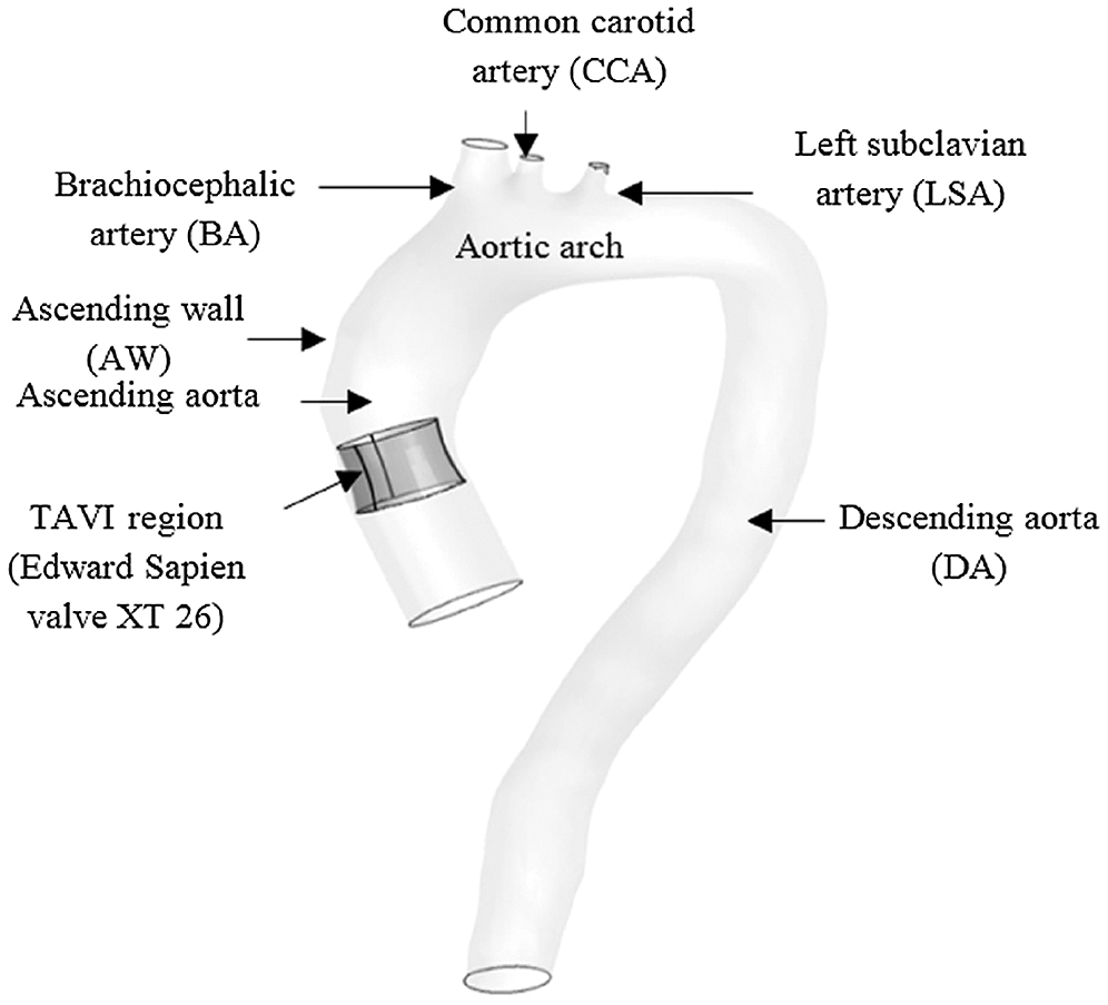
Figure 1: 3D Aorta Model with Valve using CATIA software
The location of aortic valve placement was identified and 27.3 mm annulus diameter was chosen as a reference to re-draw the TAVI valve. The 3D valve of 26 mm diameter was developed using the design data from the manufacturer, the Sapien XT (Edward SAPIEN Aortic Valve; Edwards Lifesciences, Irvine, California), as depicted in Fig. 2a [35]. The undersized of 26 mm TAVI valve was selected to indicate the presence of PVL at the aortic annulus. In this study, the TAVI leaflet was drawn at 100% GOA valve openings as in Fig. 2b.
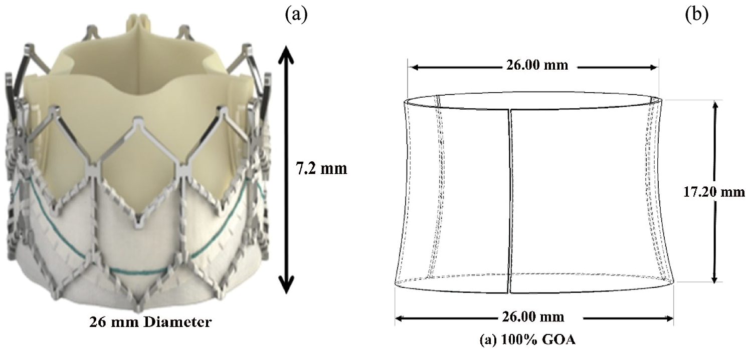
Figure 2: (a) 26 mm diameter of Sapien XT (Edward SAPIEN Aortic Valve; Edwards Lifesciences, Irvine, California) (b) 3D geometrical drawing of TAVI 26 Sapien XT with 100% GOA opening
The Navier-Stokes equation is the keystone of fundamental governing mathematical statements of the conservation laws of fluid dynamics. This Navier-Stokes equation is essentially applied to the blood flow simulation taking into account the assumptions of incompressible, turbulent, homogenous, and Newtonian flow. In this research, the body forces and energy equation were neglected as this study disregard any thermal information. Hence, considering the incompressible fluid assumption, the mass and momentum conservation equations are, as follows [36–40]:
Continuity Equation
Momentum Equation
where
Flow fields produced by different valve opening are characterized in terms of viscous shear, vorticity and Reynold shear stress [39].
In this case, the vorticity and viscous shear stress are calculated based on the spatial gradient on the mean velocity field. Both parameters are determined from the identified regions which dominated by viscous effects. While, Reynold shear stress is applied to calculate the contribution of turbulence to the mean flow.
The Navier Stokes equations of CFD in FLUENT software used the finite volume method as the numerical method solver for the discretization process [41,42]. The finite volume method utilized an integral form of conservation laws directly into a smaller sub-domains of finite number known as control volume. The advantages features of finite volume methods are the conservation properties and it is not limited to a single grid type. Hence, it provides freedom for structured and unstructured meshes [11,43].
In the model transport equations of k-ω Shear Stress Transport (SST) are solved for turbulent kinetic energy, k and ω is defined as ω = ε/k. The Transport equation of the k-ω Shear Stress Transport (SST) model as follows [44]:
where
where y is the distance to the next surface while
Model constant are:
The finite element method of the transient dynamic analysis is adopted in the structural dynamics of solid domains in order to study the structural behavior under the applications of loads [45,46]. This conversion of finite elements is interconnected at the nodes with the degree of freedom. Then, the element force vector, stiffness matrix and mass matrix are determined in a mesh by taking into account the relationship between the inertia force–acceleration and force-displacement for each element, as follows [45–49]:
where
Hence, the values of each element are connected and assembled in the form of the transformation matrix (Boolean matrix contains zeroes and ones) to the global finite element. These elements are allocated at the global matrices and organized based on the number of each element. The global stiffness, mass matrices, and applied force are evaluated as follows in Eq. (18–20), respectively [45–49]:
where A = operator responsible for the assembly process, N = number of elements, and p = force vector of a function of time.
Thus, the basic governing equation of motion can be solved for u(t) based on the response of the system called nodal displacement values using iterative methods.
From the mentioned fundamental FE equation for solid domains, it is important to update the stiffness matrix for every time step. In this case, the transient dynamic involves the structural response of impulse load that acts on the structure with a higher magnitude at a short interval of time. Using the Newmark method, the displacement is updated at every time interval followed by the stiffness matrix that is solved using a direct solver for every time step. Hence, the transient dynamic equation of the basic governing equation of motion for the structure is written as Eq. (21) [45,48].
For the FE equation of solid domains, the Newmark method is used to ensure the displacement is updated at every time interval followed by the stiffness matrix for every time step. In this case, the transient dynamic involves the structural response of impulse load that acts on the structure with a higher magnitude at a short interval of time. The basic governing equation of motion for the transient dynamic equation is written as Eq. (21) [45–49]:
where
2.3.3 Fluid-Structure Interaction Equation
Commonly, FSI is always associated with complex problems. It involves the discretization of the mathematical model related to time and space as well as the time integration concerning both domains of fluid flow and structure in order to form the system of algebraic equations. The analysis consists of two-way load transfer at the interface which is from the fluid and structure that leads to the change in boundary conditions. Moreover, the analysis is also required to update the mesh at each step until the whole simulation is successful.
The conservation of mass equation in the fluid remains the same. However, the general momentum equation is unsuitable in the transient analysis due to the frequent changes of the solution domain every time, thus induces the grid to be updated in order to change the flow boundary [50]. As mentioned previously, the ALE formulation is broadly used in the applications of vascular blood flow [42–44, 51–53]. Based on the ALE grid formulation, a relative velocity that links the actual fluid velocity to the mesh velocity is taking the place of the actual fluid velocity with respect to a fixed mesh. Hence, this requires the grid to be updated all the time referring to the modified momentum equation as shown in Eq. 22 for the denoted ith element:
where
2.4.1 Fluid Domain Boundary Condition
In this simulation, the mass flow rate and pressure are selected as the inlet and outlet with the condition of pulsatile blood flow, as referring to Lantz et al. [54] and Basri et al. [5] (as in Figs. 4a and 4b). The Newtonian and incompressible flow is assumed to be the inlet flow in this simulation due to the higher relative shear rate ratio above 100 s−1 [55]. The value of viscosity and blood density are 0.0035 Pa/s and 1050 kg/m3, respectively [9,56–61]. The Reynolds number is calculated to be 5996.92 and therefore, the flow in this study is indicated as turbulent flow. The k-ω Shear Stress Transport (SST) is selected as the turbulence model in this simulation as referred to Lantz et al. [54], Brown et al. [59] and Basri et al. [5]. The mathematical model of k-ω Shear Stress Transport (SST) is explained in Section 2.3.1.
The method used in this CFD simulation is the Coupled Algorithm for the pressure-velocity scheme which offers an alternative to the pressure-based and density-based segregated algorithm with SIMPLE-type pressure velocity coupling [62]. The Least Square Cell-Based gradient, Second Order Pressure, Second-Order Upwind Momentum, Turbulent Kinetic Energy and Specific Dissipation Rate, respectively. The time step of 0.01 s with the simulation time of 3 s (for three completed cardiac cycles) is selected in this study, by considering the small percentage difference of 6% between the time steps of 0.01 s, 0.005 s and 0.0025 s. The solution converged at 10−6 and the final pulse which is selected as the main mass flow rate inlet and pressure outlet [9,60,61]. It took about 168 h to complete the simulation using the workstation with the configuration of Intel® Core ™ i7-3520M CPU @ 2.90 GHz and 32GRAM. Hence, the four time points of pulsatile flow are taken as the reference point in this study in order to observe the fluid flow behavior. Those points are early systole (ES), peak systole (PS), early diastole (ED) and late diastole (LD), as depicted in Figs. 3a and 3b.
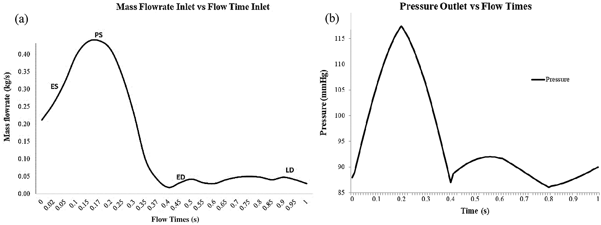
Figure 3: (a) Mass flowrate inlet consist of early systole (ES), peak systole (PS), early diastole (ED) and late diastole (LD). (b) Blood pressure pulse that used as output condition
2.4.2 Solid Domain Boundary Condition
This research generates the FSI model by adopting the linear elastic model incompressible with isotropic Young Modulus, as studied by Lantz et al. [54]. In this study, the aortic wall is assumed to be linear elastic with a density of 1080 kg/m3 and Poisson’s ratio of 0.499 [58]. The thickness of the aortic wall is assumed to be 1.5 mm (approximately 6% of the aortic diameter) [54]. The isotropic Young Modulus of 1MPa is chosen, as reported by [39,41,44,48,63]. The geometry is constrained in the axial direction at the inlet, main outlet and branch outlets as fixed supports for the aorta (refer Fig. 4). The linear elastic support of 75 mmHg pressure is applied surrounding the aorta wall to produce a natural deflection of the aorta as referred by [5,54,64]. It also helped to eliminate the high-frequency modes of structural deformation [65].
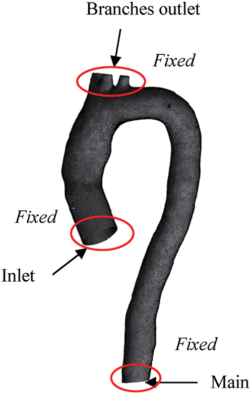
Figure 4: Boundary condition of fluid and solid domain
2.4.3 Fluid-Structure Interaction (FSI)
The FSI simulation is commonly known as the interaction between the fluid and solid interfaces of two-way coupled with the implementation of the immersed boundary method [66]. In this FSI simulation, the two-way coupling is adopted, due to its strong coupling that provides more accurate results of fluid domain concerning the feedback required by the displacements from structural deformation to the fluid simulation subjected to the moving boundary condition.
In performing the FSI analysis, system coupling is adopted as the coupling connections between participants of component systems such as fluid and solid; the coupling was either one-way or two-way. In this case, CFD played the role of participant 1 and FEA acted as participant 2 in the system, by which either the participants were receiving or feeding data in the coupled analysis. The workflow of this system coupling is simplified and depicted in Fig. 5.
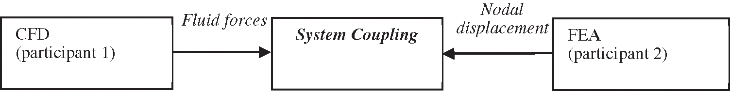
Figure 5: Work flow FSI simulation using system coupling 45
Primarily, the information from both participants 1 and 2 are collected by the system coupling to match with the complete simulation set up. Then, the obtained information is accepted before being transferred to the respective participant. The process continued with organizing the sequence of information to be exchanged by taking into account the solution part for the coupling. The final step is the convergence of coupling being assessed at the end of each of the coupling iterations.
The two-way coupling selected for this study showed a more intrinsic solving facility. During the coupling step, CFD achieved a converged solution referring to its fluid convergence before transferring the fluid forces to FEA. For the same time step of coupling, CFD also provided the solution to obtain the displacement value from structural deformation. The two-way coupling took place by which the calculated structural deformation in FEA was exchanged to CFD, so that the nodal displacement of the previous time step can help in determining a new set of fluid forces. Thus, this explained the coupling iteration which was kept on until it reached the convergence criterion of data transfer.
The grid dependency study was carried out for both fluid and solid domains as the main reference aorta without valve (AWoV) model. The relationship between the size of the mesh element and the result of maximum velocity and maximum wall shear stress are compared in order to determine the best selection of mesh elements for both fluid and solid domains. It can be concluded that, for the fluid domain, 2 million tetrahedral elements are the best mesh element while 75, 000 quadrilateral elements are considered sufficient for the case of the solid domain. The dependency graph of mesh, as depicted in Fig. 6.
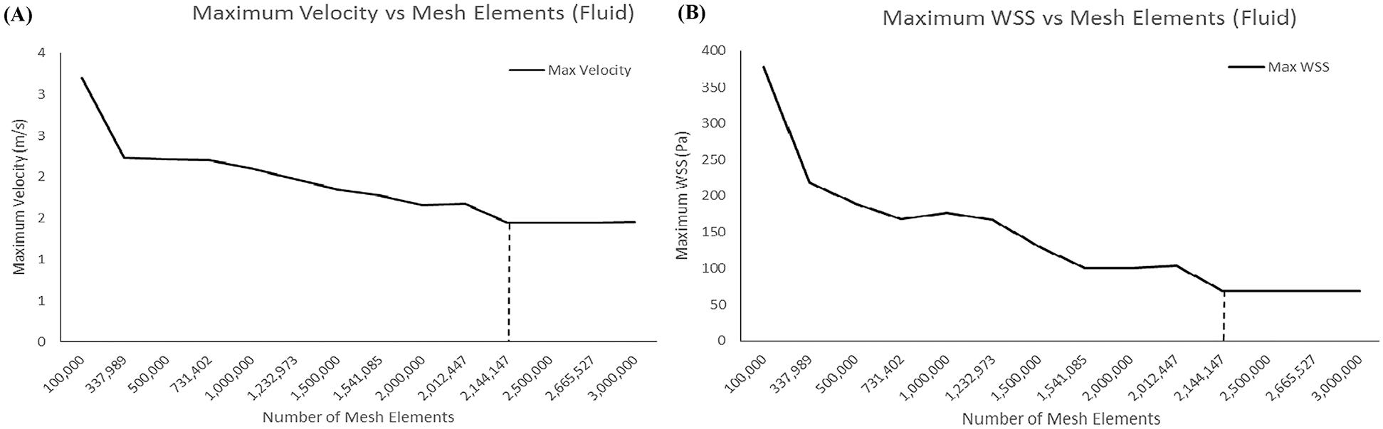
Figure 6: Result of meshes (a) Maximum velocity for fluid mesh-dependence (b) Maximum WSS for solid mesh-dependence
Referring to Fig. 7, the mass flow rate at the ascending aorta was validated by comparing with the study by Lantz et al. [54] where the graph showed the similarity pattern for both the FSI study and Lantz et al. [54] of the entire cardiac cycle. A small change in the graph pattern was noticed, which is due to the effect of different patient-specific geometry between both data and also FSI effects. Hence, it is considered acceptable to be used for the FSI study.
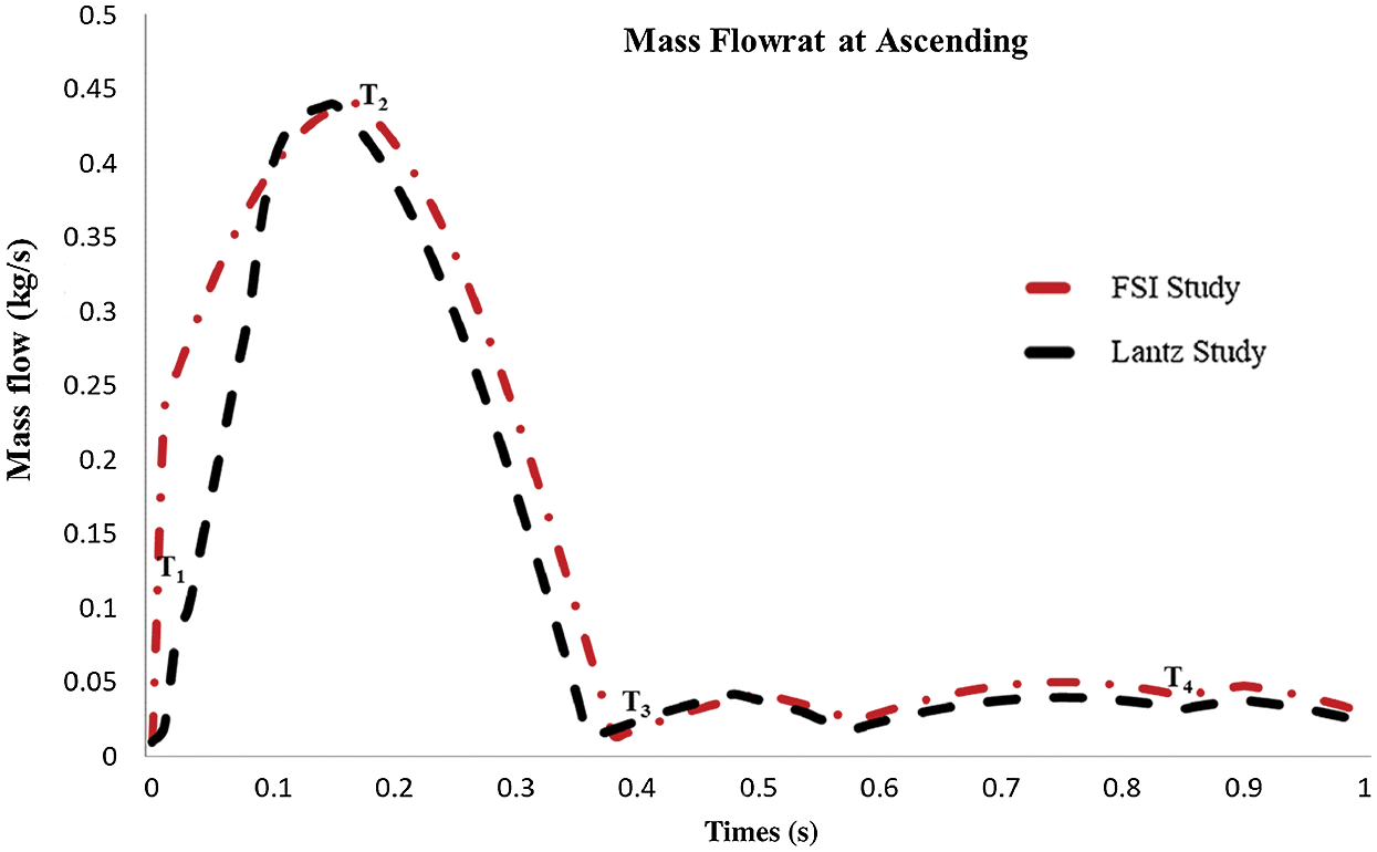
Figure 7: Mass flow rate at ascending aorta
3.2 Flow Distribution in AWoV and AWT
The velocity profile of the aorta without valve (AWoV) and aorta with TAVI 26 for 100% GOA (AWT) was captured in four different states. The ES time instance was at t = 0.02 s, PS at t = 0.17 s, ED at t = 0.37 s, and LD at t = 0.90 s for one cardiac cycle. The development and orientation of flow profiles for both aorta conditions will be discussed in the following sub-sections. The prevalence of flow distribution can be explained in Fig. 8 which represents the velocity visualization studies for both conditions of the aorta at different states. Overall, the graph of maximum velocity for both AWoV and AWT for a cardiac cycle is shown in Fig. 9.
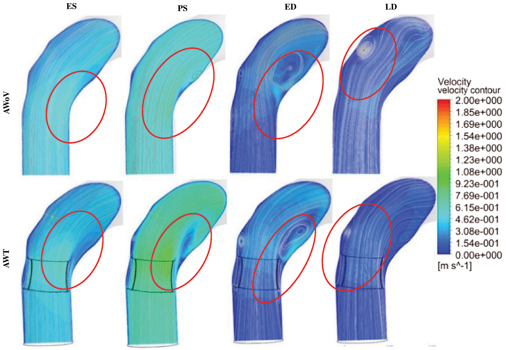
Figure 8: Velocity contour and streamlines for AWoV and AWT
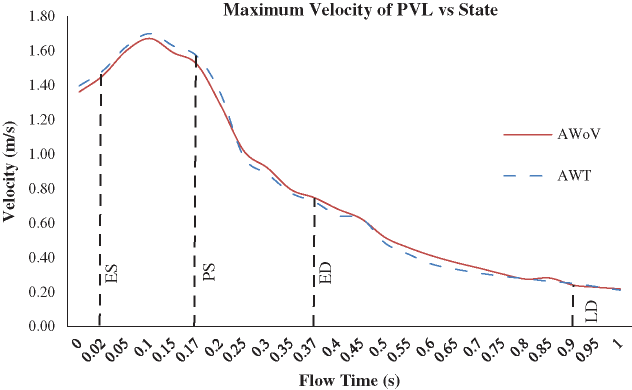
Figure 9: Maximum velocity of AWoV and AWT for one cardiac cycle
Referring to Fig. 7, at the ES state, it is observed that the light blue colour of velocity contour at the aortic annulus region of AWT produced a higher contour value compared to the AWoV. The flow is focused on the centre of the valve opening for AWT, which is a significantly higher velocity contour compared to AWoV. Quantitatively, as shown in Fig. 8, at ES state, the maximum velocity for AWoV is stated to be 1.46 m/s, while AWT shows the maximum velocity value as 1.49 m/s. The percentage difference was calculated to be 2.00% and it was observed that AWT showed a higher value compared to the AWoV.
Besides that, at PS state, the AWoV velocity streamlines showed a smooth line at the beginning of the ascending aorta before it was skewed at the inner wall of the ascending aorta towards the aortic arch region. Referring to Fig. 7, the velocity contour of AWT produced a higher value than AWoV, especially at the centre of the valve opening. It was observed that the blood flow passed through the PVL region and produced bigger recirculation flow due to the confluence of high-velocity and low-velocity proximal to the inner wall of the ascending aorta. The data in Fig. 8 showed the maximum velocity for AWT stated to be 1.57 m/s, which is 3.08% higher than the maximum velocity of AWoV with 1.52 m/s at PS state.
At the ED state, the flow distributions of AWoV and AWT are comparable with the flow distributions at the PS state. During this state, the recirculation flow patterns in the ascending aorta proximal to the aortic arch and descending aorta were amplified but produced a lower velocity magnitude compared to the previous states. Hence, the maximum velocity is stated to be 0.75 m/s and 0.72 m/s for the respective AWoV and AWT. The percentage difference between both conditions is calculated to be 3.27% in which AWoV had a higher value than AWT.
The final state of LD depicted an amplified recirculation flow pattern in the entire aorta but produced a lower velocity magnitude compared to the ES state. Referring to Fig. 7, the AWoV shows a bigger recirculation flow proximal to the outer wall of the ascending aorta. However, AWT produced another recirculation flow proximal to the inner wall of the ascending aorta, which not occurred in the AWoV condition. Thus, as shown in Fig. 8, the maximum velocity of AWoV and AWT is stated to be 0.24 m/s and 0.25 m/s, respectively. The percentage difference is calculated to be 4.20%; hence, it is indicated as the lower maximum velocity of the AWoV compared to AWT.
3.3 Pressure Distribution of AWoV and AWT
Besides that, the pressure distribution is explained from the study of pressure drop and pressure contour of both aorta conditions. Tab. 1 shows the percentage of pressure drop for AWoV and AWT. The pressure value is taken at two locations: the downside of the TAVI valve and the upper side of the valve during PS state. The value differences between both pressures are calculated to obtain the pressure drop.
Table 1: Percentage of pressure drop for AWoV and AWT
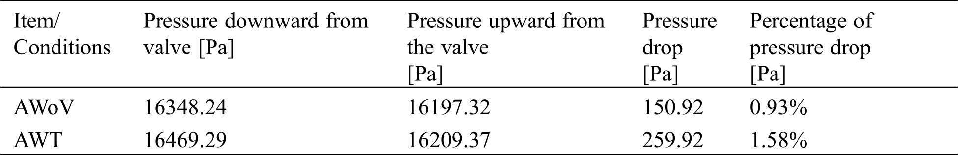
Referring to Tab. 1, the pressure drop of the AWoV is calculated to be 150.92 Pa, whereas for the AWT is 259.92 Pa. Thus, from the result, the percentage of pressure drop for the AWT is higher at 1.58% compared to the AWoV of 0.93%. Meanwhile, Fig. 9 shows the pressure contour of AWoV and AWT. The legend limit is set from 10 kPa to 18 kPa for a better comparison study. It was noticed that at ES state, the transition of green contour for AWT showed a small difference compared to the transition of green contour for AWoV (refer to red circle). During the PS state, the pressure contour showed a higher value with yellow contour for both AWoV and AWT compared to the previous state. Proximal to the inner wall of the ascending aorta, the existing light yellow spot contour for the AWT performed a bigger area compared to the AWoV. Hence, the transition of yellow contour at the aortic annulus region occurred at AWT rather than AWoV. On the other hand, at ED state, the transition of a light blue colour for AWT is lighter than the AWoV. This transition is indicated as a lower pressure value. At the final state of LD, the pressure contour of both aorta conditions does not show the difference compared to other states.
3.4 WSS Distribution of AWoV and AWT
The WSS distribution can be explained from Figs. 10 and 12 which represent the WSS visualization for both aorta conditions at different states. The WSS contour from the left and right views of both AWoV and AWT are shown in Figs. 10 and 11. The legend limit is set at a minimum of 0 Pa to a maximum of 20 Pa for a better comparison study.
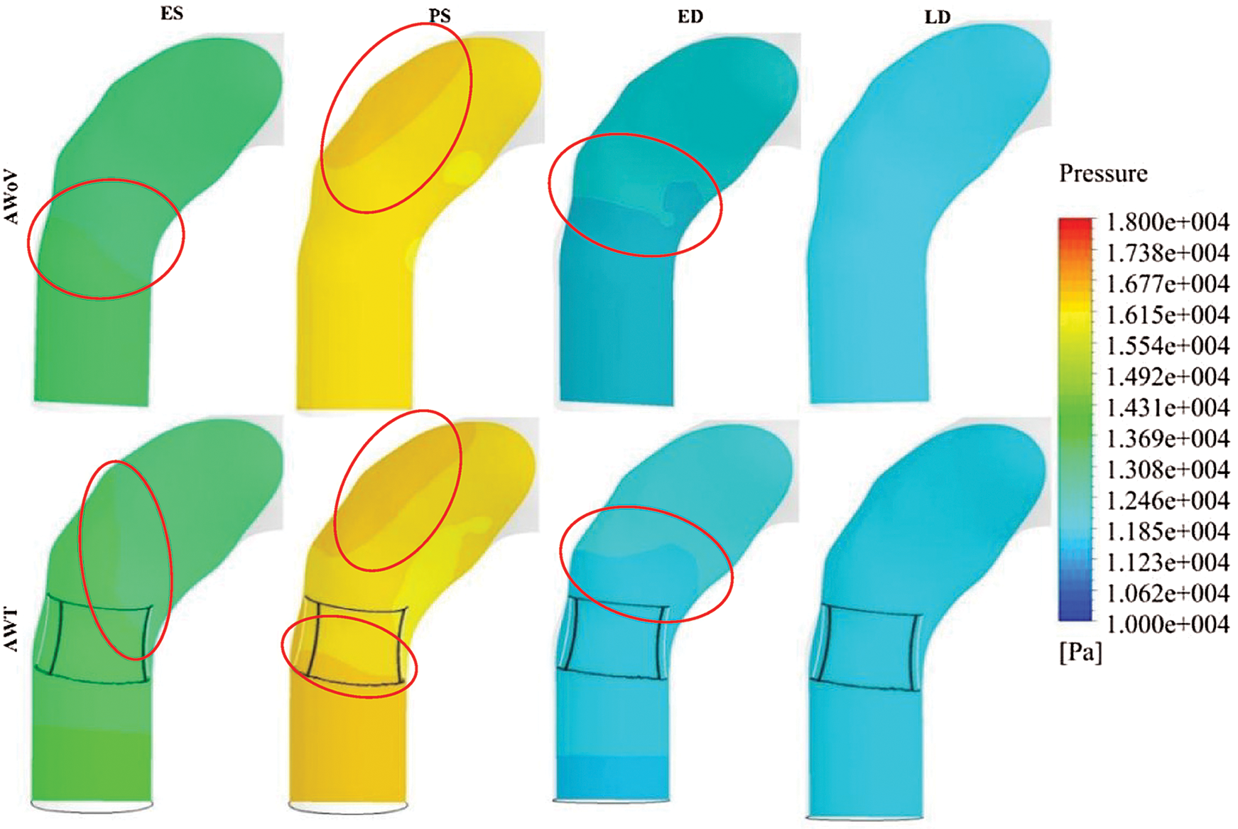
Figure 10: Pressure contour of AWoV and AWT
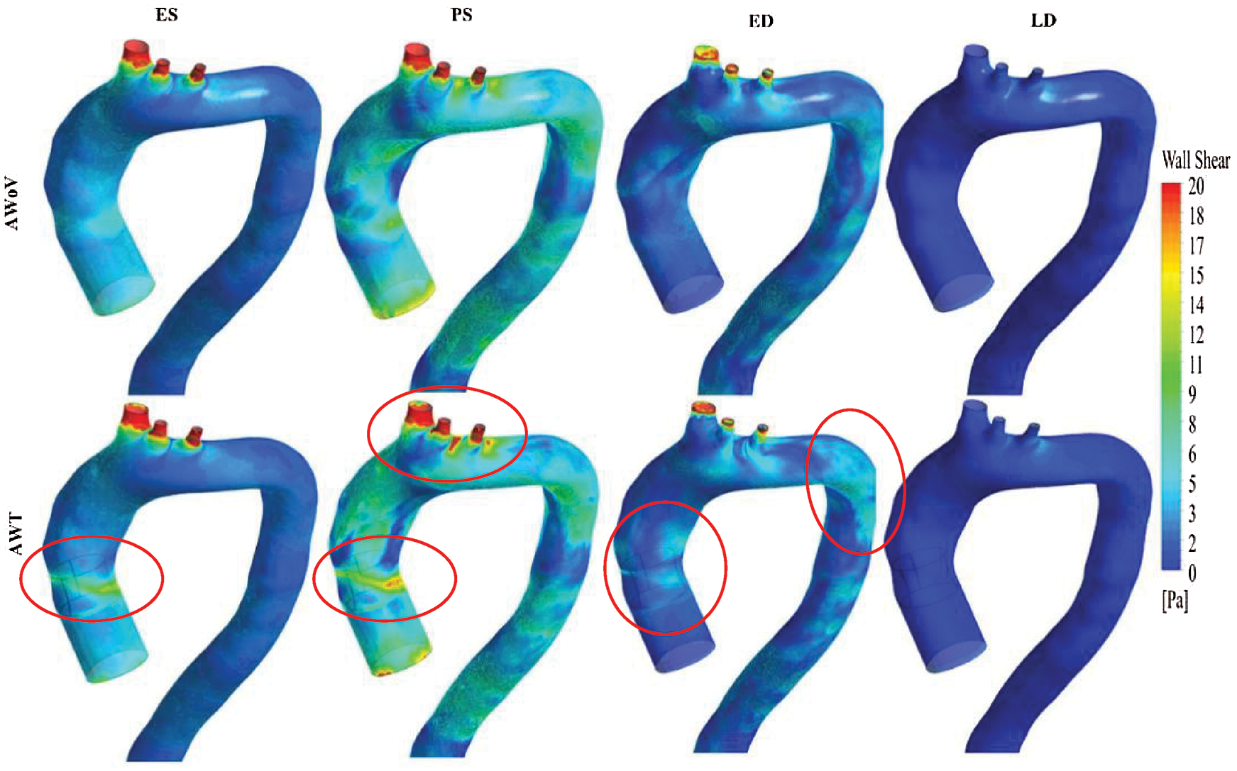
Figure 11: WSS contour from the left view of AWoV and AWT at the different states
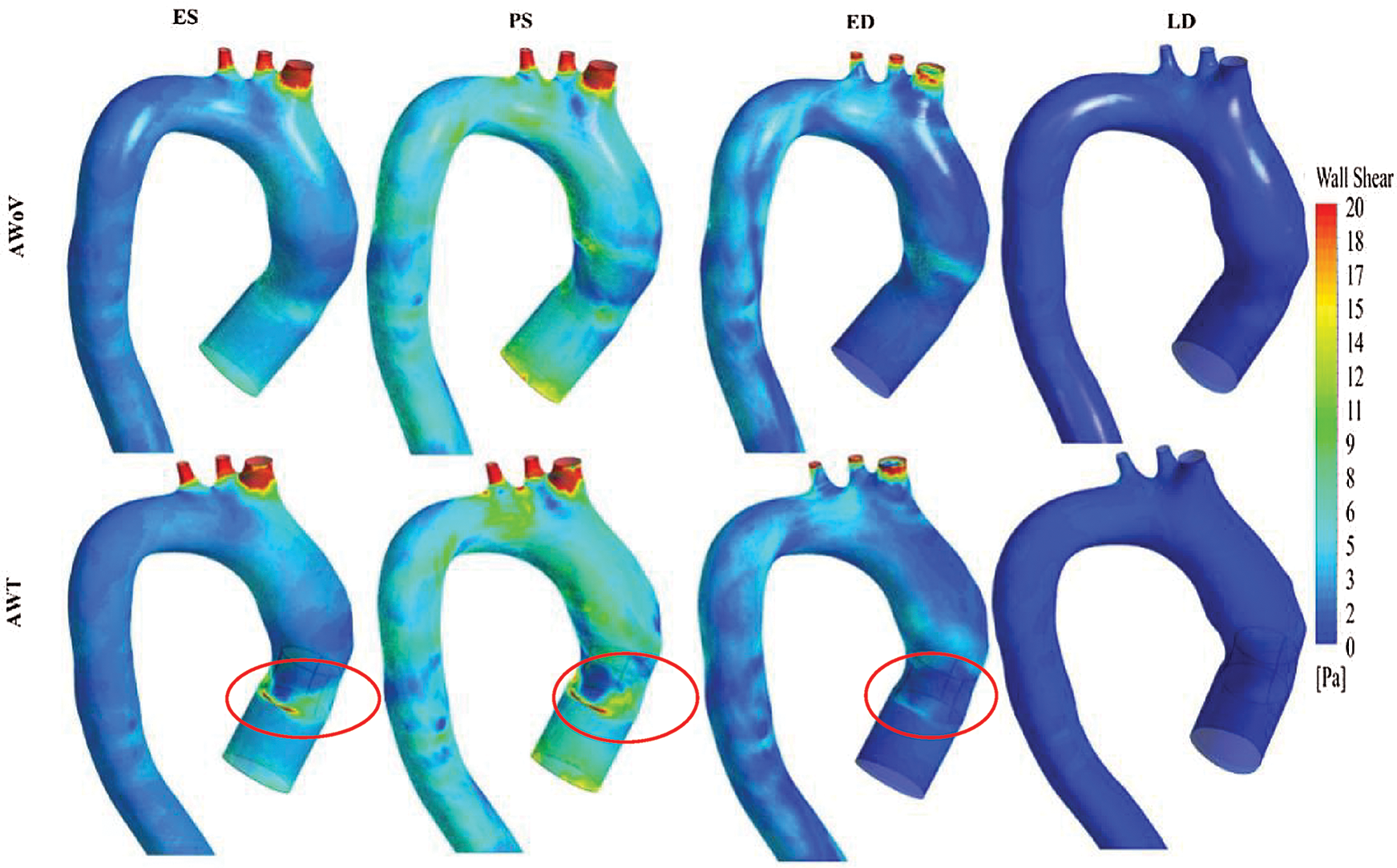
Figure 12: WSS contour from the right view of AWoV and AWT at the different states
At the ES state, the WSS contour of AWoV and AWT as shown in Fig. 10 indicated a similar contour at the aortic arch and descending aorta but a different contour in the ascending aorta. WSS in the ascending aorta for the AWoV is equally distributed compared to the AWT. The high WSS contour is concentrated proximally to the downside of TAVI at the inner wall of the ascending aorta as shown in Fig. 11. Quantitatively, referring to Fig. 12, the average WSS value of AWT at this state is 6.25 Pa, which is 87.13% higher than the WSS value of AWoV with 3.34 Pa.
At the PS state, the distributions of WSS are amplified parallel to the velocity distributions. Referring to Fig. 10, the difference of WSS effects between both AWoV and AWT occurred at the aortic arch proximal to branches and the ascending aorta proximal to TAVI. At the ascending aorta, the high value of WSS (red colour) occurred at the aortic wall surface proximal to the downside of TAVI for the AWT compared to AWoV. This consequence is due to existing of high-velocity flow at the PVL region, as shown in Figs. 11 and 12. In Fig. 12, the result of average WSS of AWT is higher than AWoV, with 8.25 Pa and 5.72 Pa, respectively. In fact, the percentage difference showed that the average WSS of AWT is 44.23% higher than AWoV.
Besides that, at the ED state, higher WSS is observed in the ascending aorta proximal to the upwards of the TAVI, as shown in Fig. 10. Higher WSS is also observed proximally to the downward of TAVI for the AWT rather than the AWoV, as shown in Fig. 11. The left view of AWT also suggested a high WSS distributed in the inner wall of the descending aorta distal from the Left Subclavian Artery (LSA) compared to the AWoV. Hence, referring to Fig. 12, the average WSS of AWT is higher than the AWoV with 3.16 Pa and 2.47 Pa, respectively. The percentage difference is calculated to be 27.94%, showing that the WSS of AWoV was lower than AWT.
At the LD state, there is no qualitative difference observed at the WSS contour of both AWoV and AWT, as shown in Figs. 11 and 12. However, as in Fig. 12a small percentage difference of WSS of 7.50% between both aorta conditions. The AWT depicts higher WSS with 0.43 Pa compared to the AWoV with 0.40 Pa.
3.5 Total Mesh Displacement of AWoV and AWT
The final element of the paravalvular effect of TAVI implantation can be explained from Fig. 14 which represents the total mesh displacement for both aorta conditions at different states. The total mesh displacement contours for both AWoV and AWT are shown in Fig. 13. The legend limit is set at a minimum of 0 mm and a maximum of 1.30 mm for a better comparison study.
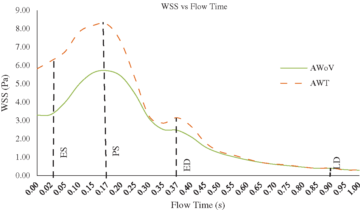
Figure 13: WSS vs. flow time of AWoV and AWT
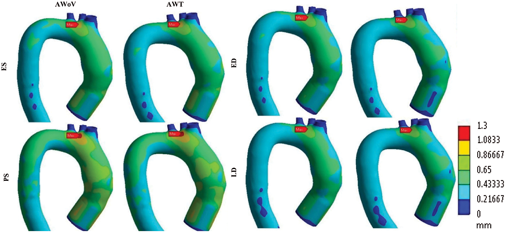
Figure 14: Total mesh displacement contour of AWoV and AWT at different states
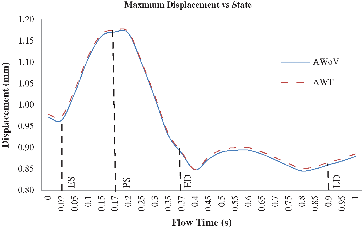
Figure 15: Maximum mesh displacement of AWoV and AWT at the different states
The maximum mesh displacement of both AWoV and AWT for one cardiac cycle is depicted in Fig. 14. A similar trend pattern is observed for both aorta conditions. Details on the total mesh displacement are discussed further.
At the ES state, the total mesh displacement distributions of AWoV and AWT exhibit a small difference between both aorta conditions. The high total mesh displacement is focused on the ascending aorta and aortic arch for AWoV and AWT and maximum mesh displacement is concentrated at the aortic arch region for both conditions. Referring to Fig. 14, the maximum mesh displacement of AWT performed a higher mesh displacement of 0.973 mm compared to AWoV with 0.964 mm. The percentage difference is calculated to be 0.93%.
At the PS state, the total mesh displacement is amplified for both AWoV and AWT. The distribution of high total mesh displacement showed similar locations for both aorta conditions. Hence, the concentration of maximum total mesh displacement of AWoV and AWT are located at the aortic arch region. The graph of maximum mesh displacement exhibits the percentage difference obtained between AWoV and AWT is around 0.34% as shown in Fig. 14. The result proved that AWT is higher with 1.175 mm compared to AWoV with 1.171 mm.
At the ED and LD states, there are no significant changes in high total mesh displacement observed between AWoV and AWT, as depicted in Fig. 13. Both states perceived the same locations of high total mesh displacement of the aorta. However, AWT showed a higher total mesh displacement of 0.889 mm compared to AWoV with 0.887 mm at the ED state. The percentage difference is calculated to be 0.23% between both aorta conditions. Meanwhile, the maximum mesh displacement of AWoV at the LD state is 0.859 mm, lower than AWT with 0.865 mm. Hence, the percentage difference obtained for both aorta conditions is 0.70%.
The PVL issue has been revealed as one of the highest complications of TAVI implantation. Thus, from the simulation conducted, the impact of leakage from mechanical properties is discussed further.
4.1 The Effects of Recirculation of Blood Flow on the Development of Blood Thrombosis
From the velocity streamlines in Fig. 7, the streamlines of AWT diverged through the centre of the valve opening at the states of ES and PS. A gap is observed between the symmetrical shapes of the TAVI valve and the asymmetrical shape of the aortic annulus, hence this causes PVL complications. Due to this matter, a huge recirculation flow is developed proximally to the inner wall of the ascending aorta, aortic arch region, and descending aorta for AWT at particular states of PS and ED. As a consequence, the velocity streamline is also reduced significantly at every state for the AWT. Furthermore, the velocity contour and streamlines of the YZ plane are amplified at the centre of the valve opening and caused the recirculation flow proximal to the inner wall of the ascending aorta. This is due to the confluence of high-velocity at the centre of valve opening and low-velocity proximal to the inner wall of the ascending aorta. Most importantly, a phenomenal backflow is observed through the PVL region for the AWT. Thus, a high maximum velocity of the AWT occurred at the states of ES, PS, and LD but low at the ED state with 1.49 m/s, 1.57 m/s, 0.25 m/s, and 0.75 m/s, respectively. From the observation, the blood flow passed through the PVL region and produced bigger recirculation flow due to the confluence of high-velocity and low-velocity proximal to the inner wall of the ascending aorta. This circumstance may cause the development of thrombus at the aorta region, which led to the blood thrombosis, as supported by Stein et al. [67].
4.2 Pressure Drop Effect on Aorta Wall Collapsed
From the pressure distribution properties in Tab. 1, the pressure difference is calculated by taking into account the pressure at the downward of the TAVI valve and on the upper side of the valve, which is 2 cm from the valve implantation at the particular state of PS. Referring to the result, AWT showed a higher pressure drop of 259.92 Pa with a percentage of 1.58% as compared to AWoV. The low-pressure contour with a bigger area of colour transition of AWT is noticed proximal to the inner wall of the ascending aorta. This finding is related to the confluence of the high and low velocity from the centre of the valve opening and PVL region, as mentioned previously. The AWT showed a higher pressure drop as compared to AWoV with a percentage of 1.58%. Hence, PVL has the highest possibility of significant pressure drop by means of the obstruction of blood flow. This consequence of pressure drop leads to high-pressure loss which augmented the flow resistance. Hence, this may cause the aorta wall to be collapsed [68–70].
4.3 WSS Effects on the Damage of Endothelium and the Potential of Aortic Rupture
From the WSS properties in Fig. 10 and 11, the AWT produced the amplified WSS from the ES to the PS states and has reduced at the states of ED to LD. A higher WSS occurred at the aortic wall proximal to the TAVI valve and branches as it reached its peak at the PS state. The increased WSS of AWT is due to the high-velocity of blood flow passing through the PVL region and divergence of the blood distributions, which disturbed the norm of the blood flow distributions in the entire aorta. In comparison with AWoV, a higher WSS of AWT is observed with the percentage difference of 87.13%, 44.23%, 27.94%, and 7.50%, for the respective states from ES to LD (refer Fig. 12). The simulation results provide the highest WSS increment at ES, PS, and LD states with 4.11, 3.21, and 3.60 of ratio difference, respectively, at the TAVI region. Thus, this effect of high-velocity flow passed through the PVL region led to higher WSS on the aortic wall surface. Thus, this effect of high-velocity flow passed through the PVL region for AWT led to higher WSS on the aortic wall surface. This also leads to the induced damage of endothelium due to the endothelial cells sensitivity and elevated level of WSS and Time Average Wall Shear Stress (TAWSS) changes [71–73]. Moreover, the aortic rupture has a high potential to be appeared on the ascending aorta wall due to the high WSS effects acting on the aorta tissue [13,74,75].
4.4 Aorta Wall Displacement Leads to the Migration of Valve
From the total mesh displacement properties in Fig. 13 and 14, both aorta conditions share similar locations of high total mesh displacement at the ascending aorta and aortic arch. Only small differences are observed between AWoV and AWT in every state. Nonetheless, the maximum mesh displacement of AWT is higher with the percentage difference of 0.93%, 0.34%, 0.23%, and 0.70% for ES, PS, ED, and LD states, respectively, as shown in Fig. 14. From the result, the AWT with the PVL issue increased the maximum mesh displacement owing to the high velocity of blood flow distribution at the aortic wall surface of the aorta. Overall, the AWT proved the seriousness of the PVL issue from various aspects of fluid mechanical properties, such as the displacement of the aorta wall may lead to the migration of the TAVI valve.
Our FSI simulation is not absent from limitations. The assumption of linear elasticity of the aorta model is restricted working strain range and more sophisticated hyperelastic material can be performed in the future for better observation. The leaflet opening is fixed at 100% GOA opening, different percentage of GOA opening can be conducted for future works in order to evaluate the effects of different percentage of GOA on the PVL complication. Moreover, the comparison of different patient geometrical can be conducted in the future for a better understanding in the effects of the different geometrical aorta.
Throughout the results obtained from the FSI simulation, the mechanical properties are compared to understand the fluid dynamics and structural deformation behavior of the patient specifics aorta model based on PVL complication. The flow behavior of velocity, pressure drop, WSS and total displacement of AWoV and AWT were compared. The findings of this study hypothesized relatively the existence of PVL at the aorta region of TAVI patient are; (a) The existence of PVL in AWT has led to the development of bigger recirculation flow proximal to the inner wall of the ascending aorta which can lead to the development of blood thrombosis at the aorta region. (b) The consequence of pressure drop may cause the aorta wall collapsed due to high-pressure loss which augmented the flow resistance. (c) High WSS magnitude of AWT along the aorta wall leads to the induced damage of endothelium and enhance the development of aortic rupture. Overall, the aid of the FSI approach is proven to be useful tools in understanding the hemodynamics and structural behavior of the development PVL in TAVI. Hence, the PVL complication leads to the development of recirculation flow, thrombus formation, aorta wall collapse, aortic rupture and damage of the endothelium.
Acknowledgement: Thank you to the co-operation and support of Department of Cardiology, National Heart Institute, Kuala Lumpur, 50400, Malaysia for this research.
Data Availability: The data used to support the findings of this study are included within the article and appendix. Raw data files of the models and simulations can be released upon application to the corresponding author (adiazriff@upm.edu.my).
Funding Statement: The authors would like to thank Universiti Putra Malaysia, for providing funds for this project through Grant UPM GP-IPM/2019/ 9675000.
Conflicts of Interest: The authors declare that they have no conflicts of interest.
1. Masson, J. B., Kovac, J., Schuler, G., Ye, J., Cheung, A. et al. (2009). Transcatheter aortic valve implantation. Review of the nature, management, and avoidance of procedural complications. JACC: Cardiovascular Interventions, 2(9), 811–820. DOI 10.1016/j.jcin.2009.07.005. [Google Scholar] [CrossRef]
2. Fanning, J. P., Platts, D. G., Walters, D. L. Fraser, J. F. (2013). Transcatheter aortic valve implantation (TAVIvalve design and evolution. International Journal of Cardiology, 168(3), 1822–1831. DOI 10.1016/j.ijcard.2013.07.117. [Google Scholar] [CrossRef]
3. Unbehaun, A., Pasic, M., Dreysse, S., Drews, T., Kukucka, M. et al. (2012). Transapical aortic valve implantation: incidence and predictors of paravalvular leakage and transvalvular regurgitation in a series of 358 patients. Journal of the American College of Cardiology, 59(3), 211–221. DOI 10.1016/j.jacc.2011.10.857. [Google Scholar] [CrossRef]
4. Vasa-Nicotera, M., Sinning, J. M., Chin, D., Lim, T. K., Spyt, T. et al. (2012). Impact of paravalvular leakage on outcome in patients after transcatheter aortic valve implantation. JACC: Cardiovascular Interventions, 5(8), 858–865. DOI 10.1016/j.jcin.2012.04.011. [Google Scholar] [CrossRef]
5. Basri, A. A., Zuber, M., Zakaria, M. S., Basri, E. I., Aziz, A. F. A. et al. (2016). The hemodynamic effects of paravalvular leakage using fluid structure interaction; Transcatheter aortic valve implantation patient. Journal of Medical Imaging and Health Informatics, 6(6), 1513–1518. DOI 10.1166/jmihi.2016.1840. [Google Scholar] [CrossRef]
6. Luu, J., Ali, O., Feldman, T. E., Price, M. J. (2013). Percutaneous closure of paravalvular leak after transcatheter aortic valve replacement. JACC: Cardiovascular Interventions, 6(2), e6–e8. DOI 10.1016/j.jcin.2012.08.026. [Google Scholar] [CrossRef]
7. Kodali, S. K., Williams, M. R., Smith, C. R., Svensson, L. G., Webb, J. G. et al. (2012). Two-year outcomes after transcatheter or surgical aortic-valve replacement. New England Journal of Medicine, 366(18), 1686–1695. DOI 10.1056/NEJMoa1200384. [Google Scholar] [CrossRef]
8. Lerakis, S., Hayek, S. S., Douglas, P. S. (2013). Paravalvular aortic leak after transcatheter aortic valve replacement: current knowledge. Circulation, 127(3), 397–407. DOI 10.1161/CIRCULATIONAHA.112.142000. [Google Scholar] [CrossRef]
9. Jahangiri, M., Saghafian, M., Sadeghi, M. R. (2015). Numerical study of turbulent pulsatile blood flow through stenosed artery using fluid-solid interaction, Computational and Mathematical Methods in Medicine,1(10). [Google Scholar]
10. Khader, S. A., Ayachit, A., Pai, B. R., Ahmed, K. A., Rao, V. R. K. et al. (2014). FSI simulation of increased severity in patient specific common carotid artery stenosis. proceedings of the 3rd International Conference on Mechanical, Electronics and Mechatronics Engineering, pp. 16–21. [Google Scholar]
11. Zakaria, M. S., Ismail, F., Tamagawa, M., Aziz, A. F. A., Wiriadidjaja, S. et al. (2019). A Cartesian non-boundary fitted grid method on complex geometries and its application to the blood flow in the aorta using OpenFOAM. Mathematics and Computers in Simulation, 159(1), 220–250. DOI 10.1016/j.matcom.2018.11.014. [Google Scholar] [CrossRef]
12. Sigüenza, J., Pott, D., Mendez, S., Sonntag, S. J., Kaufmann, T. A. et al. (2018). Fluid-structure interaction of a pulsatile flow with an aortic valve model: a combined experimental and numerical study. International Journal for Numerical Methods in Biomedical Engineering, 34(4), e2945. DOI 10.1002/cnm.2945. [Google Scholar] [CrossRef]
13. Dabagh, M., Vasava, P., Jalali, P. (2015). Effects of severity and location of stenosis on the hemodynamics in human aorta and its branches. Medical & Biological Engineering & Computing, 53(5), 463–476. DOI 10.1007/s11517-015-1253-3. [Google Scholar] [CrossRef]
14. Basri, A. A., Zuber, M., Zakaria, M. S., Illyani, E., Ahmad, A. (2016). The effects of aortic stenosis on the hemodynamic flow properties using computational fluid dynamics. International Journal of Heat and Fluid Flow, 1(3), 33–42. [Google Scholar]
15. Gsell, M. A., Augustin, C. M., Prassl, A. J., Karabelas, E., Fernandes, J. F. et al. (2018). Assessment of wall stresses and mechanical heart power in the left ventricle: Finite element modeling versus Laplace analysis. International Journal for Numerical Methods in Biomedical Engineering, 34(12), e3147. DOI 10.1002/cnm.3147. [Google Scholar] [CrossRef]
16. Zakaria, M. S., Ismail, F., Tamagawa, M., Aziz, A. F. A., Wiriadidjaya, S. et al. (2016). Numerical analysis using a fixed grid method for cardiovascular flow application. Journal of Medical Imaging and Health Informatics, 6(6), 1483–1488. DOI 10.1166/jmihi.2016.1835. [Google Scholar] [CrossRef]
17. Zakaria, M. S., Ismail, F., Tamagawa, M., Aziz, A. F. A., Wiriadidjaja, S. et al. (2017). Review of numerical methods for simulation of mechanical heart valves and the potential for blood clotting. Medical & Biological Engineering & computing, 55(9), 1519–1548. DOI 10.1007/s11517-017-1688-9. [Google Scholar] [CrossRef]
18. Zakaria, M. S., Ismail, F., Tamagawa, M., Azi, A. F. A., Wiriadidjaya, S. et al. (2018). Computational fluid dynamics study of blood flow in aorta using OpenFOAM. Journal of Advanced Research in Fluid Mechanics and Thermal Sciences, 43(1), 81–89. [Google Scholar]
19. Azriff, A., Johny, C., Khader, S. A., Pai, B. R., Zuber, M. et al. (2018). Numerical study of haemodynamics in abdominal aorta with renal branches using fluid-structure interaction under rest and exercise conditions. International Journal of Recent Technology and Engineering, 7(4), 23–27. [Google Scholar]
20. Basri, A. A., Khader, S. M. A., Johny, C., Pai, R., Zuber, M. et al. (2018). Numerical Study of haemodynamics behaviour in normal and single stenosed renal artery using fluid-structure interaction. Journal of Advanced Research in Fluid Mechanics and Thermal Sciences, 51(1), 91–98. [Google Scholar]
21. Febina, J., Sikkandar, M. Y., Sudharsan, N. M. (2018). Wall shear stress estimation of thoracic aortic aneurysm using computational fluid dynamics. Computational and Mathematical Methods in Medicine, 2018(11–12), 1–12. DOI 10.1155/2018/7126532. [Google Scholar] [CrossRef]
22. Azriff, A., Khader, S. M. A., Pai, R., Zubair, M., Ahmad, K. A. et al. (2018). Haemodynamics study in subject-specific abdominal aorta with renal bifurcation using CFD-A case study. Journal of Advanced Research in Fluid Mechanics and Thermal Sciences, 50(2), 118–121. [Google Scholar]
23. Wan Ab Naim, W. N., Ganesan, P. B., Sun, Z., Osman, K., Lim, E. (2014). The impact of the number of tears in patient-specific Stanford type B aortic dissecting aneurysm: CFD simulation. Journal of Mechanics in Medicine and Biology, 14(2), 1450017. DOI 10.1142/S0219519414500171. [Google Scholar] [CrossRef]
24. Wan Ab Naim, W. N., Ganesan, P. B., Sun, Z., Lei, J., Jansen, S. et al. (2018). Flow pattern analysis in type B aortic dissection patients after stent-grafting repair: comparison between complete and incomplete false lumen thrombosis. International Journal for Numerical Methods in Biomedical Engineering, 34(5), e2961. DOI 10.1002/cnm.2961. [Google Scholar] [CrossRef]
25. Ab Naim, W. N. W., Ganesan, P. B., Sun, Z., Liew, Y. M., Qian, Y. et al. (2016). Prediction of thrombus formation using vortical structures presentation in Stanford type B aortic dissection: a preliminary study using CFD approach. Applied Mathematical Modelling, 40(4), 3115–3127. DOI 10.1016/j.apm.2015.09.096. [Google Scholar] [CrossRef]
26. Chan, B. T., Osman, N. A. A., Lim, E., Chee, K. H., Aziz, Y. F. A. et al. (2013). Sensitivity analysis of left ventricle with dilated cardiomyopathy in fluid structure simulation. PLoS One, 8(6), e67097. DOI 10.1371/journal.pone.0067097. [Google Scholar] [CrossRef]
27. Basri, A. A., Khader, S. A., Johny, C., Pai, R., Zuber, M. et al. (2020). Effect of single and double stenosed on renal arteries of abdominal aorta: a computational fluid dynamics. CFD Letters, 12(1), 87–97. [Google Scholar]
28. Auricchio, F., Conti, M., Morganti, S., Reali, A. (2014). Simulation of transcatheter aortic valve implantation: a patient-specific finite element approach. Computer Methods in Biomechanics and Biomedical Engineering, 17(12), 1347–1357. [Google Scholar]
29. Bianchi, M., Marom, G., Ghosh, R. P., Fernandez, H. A., Taylor, J. R.Jr. et al. (2016). effect of balloon-expandable transcatheter aortic valve replacement positioning: a patient-specific numerical model. Artificial Organs, 40(12), E292–E304. DOI 10.1111/aor.12806. [Google Scholar] [CrossRef]
30. Bianchi, M., Marom, G., Ghosh, R. P., Rotman, O. M., Parikh, P. et al. (2019). Patient-specific simulation of transcatheter aortic valve replacement: impact of deployment options on paravalvular leakage. Biomechanics and Modeling in Mechanobiology, 18(2), 435–451. DOI 10.1007/s10237-018-1094-8. [Google Scholar] [CrossRef]
31. Rocatello, G., de Santis, G., de Bock, S., de Beule, M., Segers, P. et al. (2019). Optimization of a transcatheter heart valve frame using patient-specific computer simulation. Cardiovascular Engineering and Technology, 10(3), 456–468. DOI 10.1007/s13239-019-00420-7. [Google Scholar] [CrossRef]
32. Rocatello, G., El Faquir, N., de Backer, O., Swaans, M. J., Latib, A. et al. (2019). The impact of size and position of a mechanical expandable transcatheter aortic valve: novel insights through computational modelling and simulation. Journal of Cardiovascular Translational Research, 12(5), 435–446. DOI 10.1007/s12265-019-09877-2. [Google Scholar] [CrossRef]
33. Mao, W., Li, K., Sun, W. (2016). Fluid-structure interaction study of transcatheter aortic valve dynamics using smoothed particle hydrodynamics. Cardiovascular Engineering and Technology, 7(4), 374–388. DOI 10.1007/s13239-016-0285-7. [Google Scholar] [CrossRef]
34. Luraghi, G., Migliavacca, F., García-González, A., Chiastra, C., Rossi, A. et al. (2019). On the modeling of patient-specific transcatheter aortic valve replacement: a fluid-structure interaction approach. Cardiovascular Engineering and Technology, 10(3), 437–455. DOI 10.1007/s13239-019-00427-0. [Google Scholar] [CrossRef]
35. Kasel, A. M., Cassese, S., Bleiziffer, S., Amaki, M., Hahn, R. T. et al. (2013). Standardized imaging for aortic annular sizing: implications for transcatheter valve selection. JACC: Cardiovascular Imaging, 6(2), 249–262. DOI 10.1016/j.jcmg.2012.12.005. [Google Scholar] [CrossRef]
36. Náraigh, L. Ó., van Vuuren, D. R. J. (2019). Linear and nonlinear stability analysis in microfluidic systems. Fluid Dynamic & Material Processing, 16(2), 383–410. [Google Scholar]
37. Gibou, F., Min, C., Ceniceros, H. D. (2007). Non-graded adaptive grid approaches to the incompressible Navier-Stokes equations. Fluid Dynamic & Material Processing, 3(1), 37–48. [Google Scholar]
38. López, A. G., Reyes, I. P., Villa, A. L., Aguilar, R. V. (2016). Stochastic simulation for couette flow of dilute polymer solutions using Hookean dumbbells. Recent Advances in Fluid Dynamics with Environmental Applications, pp. 217–228. Springer, Cham. [Google Scholar]
39. Seaman, C., George Akingba, A., Sucosky, P. (2014). Steady flow hemodynamic and energy loss measurements in normal and simulated calcified tricuspid and bicuspid aortic valves. Journal of Biomechanical Engineering, 136(4), 72. DOI 10.1115/1.4026575. [Google Scholar] [CrossRef]
40. Tala, C. D. (2010). Numerical simulation of steady and pulsatile flow in stenosed tapered artery and abdominal aortic aneurysm using κ-ω model. (Phd Thesis). Wichita State University, UK. [Google Scholar]
41. Ferreira, A. C., Carneiro, F., Teixeira, S., Teixeira, J. C., Gama Ribeiro, V. (2009). Numerical study of blood flow in a vessel with increasing degree of stenosis using dynamic meshes. XIII Congr Internacional Ingenieria Proyectos,1(9), 1951–1960. [Google Scholar]
42. Alsuhairi, N. (2012). Fluid structure interaction-A study of pouring, using FSI-simulations (Master Thesis). Lund University, Sweden. [Google Scholar]
43. Caballero, A. D., Laín, S. (2013). A review on computational fluid dynamics modelling in human thoracic aorta. Cardiovascular Engineering and Technology, 4(2), 103–130. DOI 10.1007/s13239-013-0146-6. [Google Scholar] [CrossRef]
44. James, M. E., Papavassiliou, D. V., O’Rear, E. A. (2019). Use of computational fluid dynamics to analyze blood flow, hemolysis and sublethal damage to red blood cells in a bileaflet artificial heart valve. Fluids, 4(1), 19. DOI 10.3390/fluids4010019. [Google Scholar] [CrossRef]
45. Raja, R. S. (2012). Coupled fluid structure interaction analysis on a cylinder exposed to ocean wave loading (Master Thesis). Chalmers University of Technology, Sweden. [Google Scholar]
46. Basri, A. A., Zuber, M., Basri, E. I., Zakaria, M. S., Aziz, A. F. et al. (2020). Fluid structure interaction on paravalvular leakage of transcatheter aortic valve implantation related to aortic stenosis: a patient-specific case. Computational and Mathematical Methods in Medicine, 1(5), 1–22. [Google Scholar]
47. Chopra, A. K. (2017). Dynamics of structures theory and applications to earthquake engineering. Pearson Prentice Hall, University of Victoria Engineering, Canada. [Google Scholar]
48. Hughes, T. J. (2012). The finite element method: linear static and dynamic finite element analysis. Courier Corporation, USA. [Google Scholar]
49. Figueroa, C. A., Baek, S., Taylor, C. A., Humphrey, J. D. (2009). A computational framework for fluid-solid-growth modeling in cardiovascular simulations. Computer Methods in Applied Mechanics and Engineering, 198(45–46), 3583–3602. DOI 10.1016/j.cma.2008.09.013. [Google Scholar] [CrossRef]
50. Ferziger, J. H., Perić, M., Street, R. L. (2002). Computational methods for fluid dynamics, vol. 3. pp. 196–200. Berlin: Springer. [Google Scholar]
51. Formaggia, L., Nobile, F. (2004). Stability analysis of second-order time accurate schemes for ALE-FEM. Computer Methods in Applied Mechanics and Engineering, 193(39–41), 4097–4116. DOI 10.1016/j.cma.2003.09.028. [Google Scholar] [CrossRef]
52. Fernández, M. A., Moubachir, M. (2005). A Newton method using exact Jacobians for solving fluid-structure coupling. Computers & Structures, 83(2–3), 127–142. DOI 10.1016/j.compstruc.2004.04.021. [Google Scholar] [CrossRef]
53. Mark, A., Rundqvist, R., Edelvik, F. (2011). Comparison between different immersed boundary conditions for simulation of complex fluid flows. Fluid Dynamics & Materials Processing, 7(3), 241–258. [Google Scholar]
54. Lantz, J., Renner, J., Karlsson, M. (2012). Wall shear stress in a subject specific human aorta—influence of fluid-structure interaction. International Journal of Applied Mechanics, 3(4), 759–778. DOI 10.1142/S1758825111001226. [Google Scholar] [CrossRef]
55. Manimaran, R. (2011). CFD simulation of non-Newtonian fluid flow in arterial stenoses with surface irregularities. World Academy of Science, Engineering and Technology, 73(5), 804–809. [Google Scholar]
56. Gao, F., Watanabe, M., Matsuzawa, T. (2006). Stress analysis in a layered aortic arch model under pulsatile blood flow. Biomedical Engineering Online, 5(1), 525. DOI 10.1186/1475-925X-5-25. [Google Scholar] [CrossRef]
57. Marom, G., Kim, H. S., Rosenfeld, M., Raanani, E., Haj-Ali, R. (2012). Effect of asymmetry on hemodynamics in fluid-structure interaction model of congenital bicuspid aortic valves. 2012 Annual International Conference of the IEEE Engineering in Medicine and Biology Society, pp. 637–640. [Google Scholar]
58. Marom, G., Kim, H. S., Rosenfeld, M., Raanani, E., Haj-Ali, R. (2013). Fully coupled fluid-structure interaction model of congenital bicuspid aortic valves: effect of asymmetry on hemodynamics. Medical & Biological Engineering & Computing, 51(8), 839–848. DOI 10.1007/s11517-013-1055-4. [Google Scholar] [CrossRef]
59. Brown, S., Wang, J., Ho, H., Tullis, S. (2013). Numeric simulation of fluid-structure interaction in the aortic arch. In Computational Biomechanics for Medicine. pp. 13–23. New York, NY: Springer. [Google Scholar]
60. Jahangiri, M., Saghafian, M., Sadeghi, M. R. (2015). Effects of non-Newtonian behavior of blood on wall shear stress in an elastic vessel with simple and consecutive stenosis. Biomedical and Pharmacology Journal, 8(1), 123–131. DOI 10.13005/bpj/590. [Google Scholar] [CrossRef]
61. Jahangiri, M., Saghafian, M., Sadeghi, M. R. (2017). Numerical simulation of non-Newtonian models effect on hemodynamic factors of pulsatile blood flow in elastic stenosed artery. Journal of Mechanical Science and Technology, 31(2), 1003–1013. DOI 10.1007/s12206-017-0153-x. [Google Scholar] [CrossRef]
62. Choi, C. R., Kim, C. N., Choi, M. J. (2001). Characteristics of transient blood flow in MHVs with different maximum opening angles using fluid-structure interaction method. Korean Journal of Chemical Engineering, 18(6), 809–815. DOI 10.1007/BF02705601. [Google Scholar] [CrossRef]
63. Figueroa, C. A., Vignon-Clementel, I. E., Jansen, K. E., Hughes, T. J., Taylor, C. A. (2006). A coupled momentum method for modeling blood flow in three-dimensional deformable arteries. Computer Methods in Applied Mechanics and Engineering, 195(41–43), 5685–5706. DOI 10.1016/j.cma.2005.11.011. [Google Scholar] [CrossRef]
64. Kim, H., Lu, J., Sacks, M. S., Chandran, K. B. (2008). Dynamic simulation of bioprosthetic heart valves using a stress resultant shell model. Annals of Biomedical Engineering, 36(2), 262–275. DOI 10.1007/s10439-007-9409-4. [Google Scholar] [CrossRef]
65. Takizawa, K., Moorman, C., Wright, S., Christopher, J., Tezduyar, T. E. (2010). Wall shear stress calculations in space-time finite element computation of arterial fluid-structure interactions. Computational Mechanics, 46(1), 31–41. DOI 10.1007/s00466-009-0425-0. [Google Scholar] [CrossRef]
66. Hou, G., Wang, J., Layton, A. (2012). Numerical methods for fluid-structure interaction—a review. Communications in Computational Physics, 12(2), 337–377. [Google Scholar]
67. Stein, P. D., Sabbah, H. N. (1976). Turbulent blood flow in the ascending aorta of humans with normal and diseased aortic valves. Circulation Research, 39(1), 58–65. DOI 10.1161/01.RES.39.1.58. [Google Scholar] [CrossRef]
68. Keshavarz-Motamed, Z., Garcia, J., Pibarot, P., Larose, E., Kadem, L. (2011). Modeling the impact of concomitant aortic stenosis and coarctation of the aorta on left ventricular workload. Journal of Biomechanics, 44(16), 2817–2825. DOI 10.1016/j.jbiomech.2011.08.001. [Google Scholar] [CrossRef]
69. Ku, D. N., Zeigler, M. N., Downing, J. M. (1990). One-dimensional steady inviscid flow through a stenotic collapsible tube. Journal of Biomechnical Engineering,112(4), 444–450. [Google Scholar]
70. Tang, D., Yang, C., Kobayashi, S., Zheng, J., Vito, R. P. (2003). Effect of stenosis asymmetry on blood flow and artery compression: a three-dimensional fluid-structure interaction model. Annals of Biomedical Engineering, 31(10), 1182–1193. DOI 10.1114/1.1615577. [Google Scholar] [CrossRef]
71. Leuprecht, A., Kozerke, S., Boesiger, P., Perktold, K. (2003). Blood flow in the human ascending aorta: a combined MRI and CFD study. Journal of Engineering Mathematics, 47(3/4), 387–404. DOI 10.1023/B:ENGI.0000007969.18105.b7. [Google Scholar] [CrossRef]
72. Nabaei, M., Fatouraee, N. (2012). Computational modeling of formation of a cerebral aneurysm under the influence of smooth muscle cell relaxation. Journal of Mechanics in Medicine and Biology, 12(1), 1250006. DOI 10.1142/S0219519411004599. [Google Scholar] [CrossRef]
73. Sheard, G. J. (2009). Flow dynamics and wall shear-stress variation in a fusiform aneurysm. Journal of Engineering Mathematics, 64(4), 379–390. DOI 10.1007/s10665-008-9261-z. [Google Scholar] [CrossRef]
74. Mori, D., Yamaguchi, T. (2002). Computational fluid dynamics modeling and analysis of the effect of 3-D distortion of the human aortic arch. Computer Methods in Biomechanics and Biomedical Engineering, 5(3), 249–260. DOI 10.1080/10255840290010698. [Google Scholar] [CrossRef]
75. Wolters, B. J. B. M., Rutten, M. C. M., Schurink, G. W. H., Kose, U., de Hart, J. et al. (2005). A patient-specific computational model of fluid-structure interaction in abdominal aortic aneurysms. Medical Engineering & Physics, 27(10), 871–883. DOI 10.1016/j.medengphy.2005.06.008. [Google Scholar] [CrossRef]
 | This work is licensed under a Creative Commons Attribution 4.0 International License, which permits unrestricted use, distribution, and reproduction in any medium, provided the original work is properly cited. |