Materials Processing
| Fluid Dynamics & Materials Processing |
DOI: 10.32604/fdmp.2021.015082
ARTICLE
A Research on the Flow Characteristics of a Splitter-Based Water Cooling System for Computer Boards
North China Electric Power University, Baoding, 071003, China
*Corresponding Author: Quanzhi Ge. Email: Gequanzhi@126.com
Received: 20 November 2020; Accepted: 08 March 2021
Abstract: The splitter is an important component of water-based cooling systems used to extract heat from computer boards. In the present study, the flow characteristics of a 16-splitter structure were numerically simulated and compared with experimental results to verify the reliability of the numerical simulation method. Accordingly, the concept of splitter structural coefficients was proposed. Based on the results of this study, we recommend a selection range of 5 ≤ k ≤ 6 for the structure factor k of the splitter; after optimization, the maximum deviation of the splitter outlet flow was reduced from the original value of 100% to 8.3%.
Keywords: Computing board; cold-water splitter; structure factor; flow-transfer characteristics; experimental study; numerical simulation
The development of new technology has improved the performance of electronic instruments, increasing their power densities and reducing their sizes. Consequently, the heat flow generated by the electronic equipment has increased [1]. Although the computing board has a strong calculating ability, it generates a large amount of heat [2–5], affecting its performance. The two currently available methods for dissipating the heat of the computing board are air and water cooling.
In air cooling, a fast-rotating fan blows air directly into the heat source to dissipate the heat [6,7]. For this process, the heat-dissipation effect is significant, the installation is simple, the equipment needed is small, and the costs are low; however, the effects of the environmental conditions are significant. If the ambient temperature increases sufficiently or the equipment operates in the overclock mode, the heat-dissipation effect is reduced, and the fan generates noise because of its high rotational speed; therefore, under these conditions, the equipment is not appropriate if low noise is required.
In water cooling, circulating water is pumped to the board, passing near the computing plate, to conduct the heat generated by the computing board. The system used in this procedure is composed of a splitter, water-cooled board, pump, and heat sink [8,9]. Consequently, the working noise is low, the heat dissipation is stable, and there are few environmental constraints. Furthermore, the heat-dissipation efficiency of this system is higher than that obtained with the air-cooling equipment, as the heat-transfer coefficient is 100–1000 times larger. However, the sharing effect of the splitter matched with the water-cooling board results in uneven cooling of the board.
Although both methods have disadvantages, the water-cooled heat-dissipation method is frequently selected owing to its high heat-dissipation effect and low noise, as noise reduction is frequently demanded by users; therefore, it is a development trend.
To effectively cool the computer chip while operating with minimal noise, a single-phase water-cooled radiator of the computer chip—driven by a voltage pump with two parallel cavities—was developed [10]. Xu et al. [11] developed a numerical simulation method that considers the heat exchange and pressure loss of water-cooling plate radiators of different structural forms. Using this technique, the effects of the internal structure layout on the heat-exchange characteristics were determined. Gao et al. [12] studied the flow distribution at each outlet of three different splitters, i.e., a jin-type splitter, a conical splitter, and a reflective splitter, at different installation angles and fluid flow rates to examine the effects of these parameters on the flow-sharing effect of the splitter.
Currently, water-cooling technology has significant advantages for heat dissipation. However, owing to the development of water-cooled heat-dissipation technology for computer boards, the flow-sharing effect of the shunt must be improved. Furthermore, the numerical simulation of the macro-fluid flow must be further explored compared with the cutting-edge numerical simulations of the micro-fluid flow [13–15].
To improve the matching effect of the shunt and the water-cooled board, water-cooling technology must be deeply analyzed [16,17]. Therefore, in this study, the flow characteristics of the internal flow field of a combined computing-board water-cooled splitter were analyzed via numerical simulations and experiments. Furthermore, the flow regularity was investigated to improve the flow-sharing effect and determine the optimal model for this equipment.
The simulation software program Fluent is widely employed in diverse fields, e.g., aerospace, biology, and energy [18,19], as it offers a variety of grid types (including structural and non-structural), which can be applied before executing the simulation; physical models, such as laminar flow, turbulence, and transmission models; and different types of boundary conditions, e.g., for the inlet/outlet and wall. When executing the numerical simulation, the user can monitor the change in each physical quantity, e.g., speed, temperature, or pressure, in real time while the software performs the calculation according to a set of predefined constraints. At the end of the numerical simulation, the results can be conveniently and directly viewed. Consequently, Fluent was selected to perform the simulation.
The laws of conservation of mass and momentum are the first and second of the three conservation laws of fluid motion, respectively.
In this study, the computational and image display modules in computational fluid dynamics [20] were used to obtain the flow field at different timesteps, allowing the flow-field distribution inside the shunt to be analyzed.
Assuming that an incompressible fluid is a continuous medium, the mass flowing into a control body must be equal to the mass flowing out of the same control body [21], as follows:
where
The fluid flows also respect the law of momentum conservation.
Here,
The realizable k-ε turbulence model has high accuracy for predicting planar flows and wake diffusion relative to the other turbulence models. Furthermore, the accuracy of this model for predicting the vortex, streamline, and streamline bending and rotation is higher than that of the RNG k-ε and standard k-ε models. Owing to the complex internal structure of the shunt, the broad variations in the flow characteristics, and the fact that the cooling of the force plate is calculated in the shunt, a high accuracy is required. Consequently, considering the accuracy requirements and computer costs, the realizable k-ε turbulence model, which is given by Eq. (3), was selected to simulate the turbulence splitter [22].
Here, ρ represents the fluid density (in kg/m3); xi and xj are the coordinate components; ui and uj are the average relative velocity components; Cμ is the viscosity coefficient; k represents the turbulent kinetic energy (in m2/s2); ε represents the turbulent dissipation rate (in m2/s3); μt and μ represent the turbulent force viscosity and hydrodynamic viscosity (in Pas), respectively; σk, σε, C1, and C2 are constants whose values are 1, 1.3, 0.43, and 1.9, respectively; and pk represents the turbulence production due to the mean velocity gradients (in W/m3).
3 Comparative Analysis of Original Splitter Experiment and Simulation Results
3.1 Original Splitter Experimental System and Measurement Method
Fig. 1 shows a sketch of the original experimental system. The flow divider had a one–four structure, and the angle between the directions of the water inlet and the four water outlets was 90°. The inner diameters of the water inlet, water outlet, and shunt chamber were 10, 8, and 11 mm, respectively. Fig. 2 shows the dimensions of the original splitter.
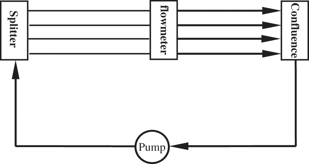
Figure 1: Original splitter experimental system diagram
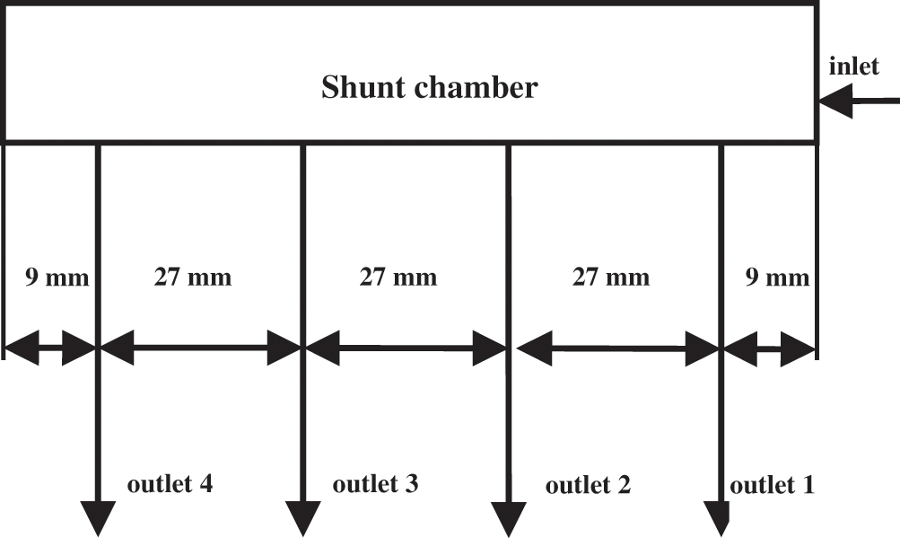
Figure 2: Schematic diagram of the center distance structure of the original splitter outlet
Assuming an intake flow of 4 L/min, a flow meter was used to measure the flow at each outlet after it was stable. The experiment was repeated five times, and the average flow at each outlet was calculated to analyze the sharing effect of the original splitter, as shown in Fig. 3. The deviation of the flow rate between the outlets was significant; the minimum and maximum flow rates were 0.6 and 1.2 L/min, respectively, corresponding to a difference of approximately 100% of the minimum flow rate.
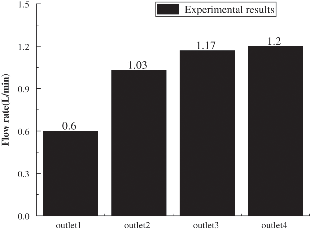
Figure 3: Experimental results of original splitter
3.2 Physical Modeling and Meshing of Original Splitter
To fulfill the technical requirements and facilitate the numerical simulation, the physical model of the original splitter was simplified, as shown in Fig. 4.
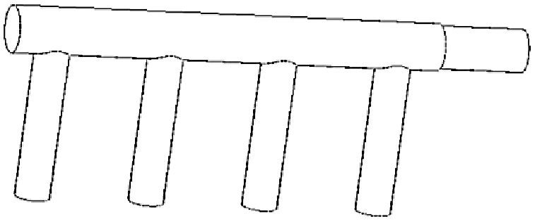
Figure 4: Physical model of the original splitter
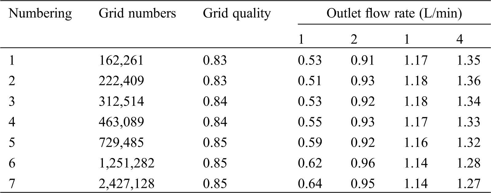
To achieve independence between the simulation results and the grid of the physical model, the grid having the highest grid quality and smallest grid number was selected for the simulations. As shown in Tab. 1, grid 6, whose number of grids was approximately 1.25 million, was selected. For subsequent splitter simulation schemes, a similar treatment was adopted.
Table 1: Verification of the grid independence of the original splitter
3.3 Single-Value Condition Setting
To use the same inlet flow rate that was employed in the experimental setup, the following conditions were set.
1. Water density at 25°C: 997.74 kg/m3
2. Dynamic viscosity: 0.894 × 10⁻³ Pa·s
3. Inlet boundary condition: velocity inlet was set as 0.85 m/s
4. Outlet boundary conditions: pressure outlet
5. Wall condition of flow channel: standard wall boundary
6. Turbulent flow model: realizable k-ε model, simple algorithm, second-order upwind discrete format
7. Initialization: hybrid
These conditions were used because water is an incompressible fluid at 25°C, and the flow is a steady-state process; accordingly, the SIMPLE algorithm [23,24] was selected. To improve the simulation accuracy, the second-order upwind discrete format was selected.
3.4 Comparative Analysis of Results of Experiment and Simulation
Fig. 5 shows a chart comparing the results of the original splitter experiment and the simulation. The flow change trends for all the outlets were similar between the experiment and the simulation, as the relative deviation of the flow rate of each outlet was <8%. Although the deviations between the simulation and experimental results were not negligible, the simulation results accurately represented the flow magnitude and deviation degree of the outlets, validating the numerical simulation method and the physical model adopted in this study.
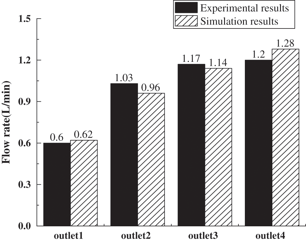
Figure 5: Comparison of experimental and simulation results
The deviations between the experimental and simulation results were attributed to the following factors. (1) The numerical simulation grid may not have been sufficiently refined, leading to a low grid quality; (2) there was a counting deviation in the original splitter experiment, where the measurement accuracy of the flowmeter (Keyence FD-81) was 0.1 L/min.
The small inner diameter of the shunt chamber resulted in a low pressure-balancing effect; therefore, the water in the shunt chamber flowed toward outlet 4, as it was the farthermost outlet. Furthermore, the inner diameter of the outlet was large; therefore, the flow resistance was small. Consequently, the flow rates at outlets 1 and 4 were low and high, respectively. According to this preliminary analysis, the poor shunt effect may have been due to (1) the small inner diameter of the shunt chamber or (2) the large inner diameter of the outlet. This conclusion can be used to optimize the geometry of the shunt.
4 Structural Improvement Scheme and Numerical Simulation Analysis
4.1 Structural Improvement Scheme
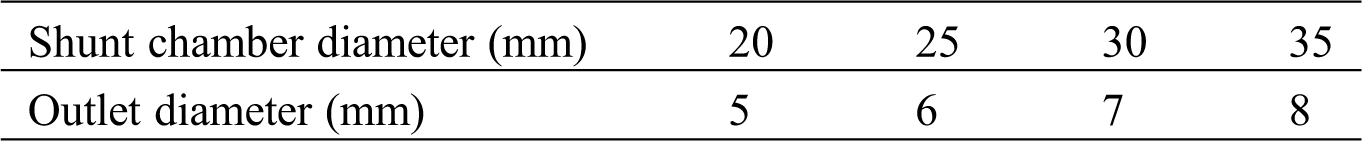
Assuming that the center distance of the water outlet of the flow splitter was preserved, the internal diameter of the shunt chamber and water outlet were changed to investigate the flow shunt behavior through numerical simulations. From the parameters presented in Tab. 2, 16 structural improvement schemes were designed.
Table 2: Structural improvement schemes
4.2 Numerical Simulation Analysis
Physical models were established for each structural improvement scheme. Single-valued conditions similar to those established in Section 2.3 were used to execute the numerical simulations. The central cross section was selected as a velocity cloud to analyze the shunt effect. Figs. 6 and 7 show comparisons between velocity cloud diagrams for cases where the inner diameters of all the outlets were 5, 6, 7, and 8 mm and 20, 25, 30, and 35 mm and the inner diameters of the shunt chamber and the outlet were 25 and 6 mm, respectively.
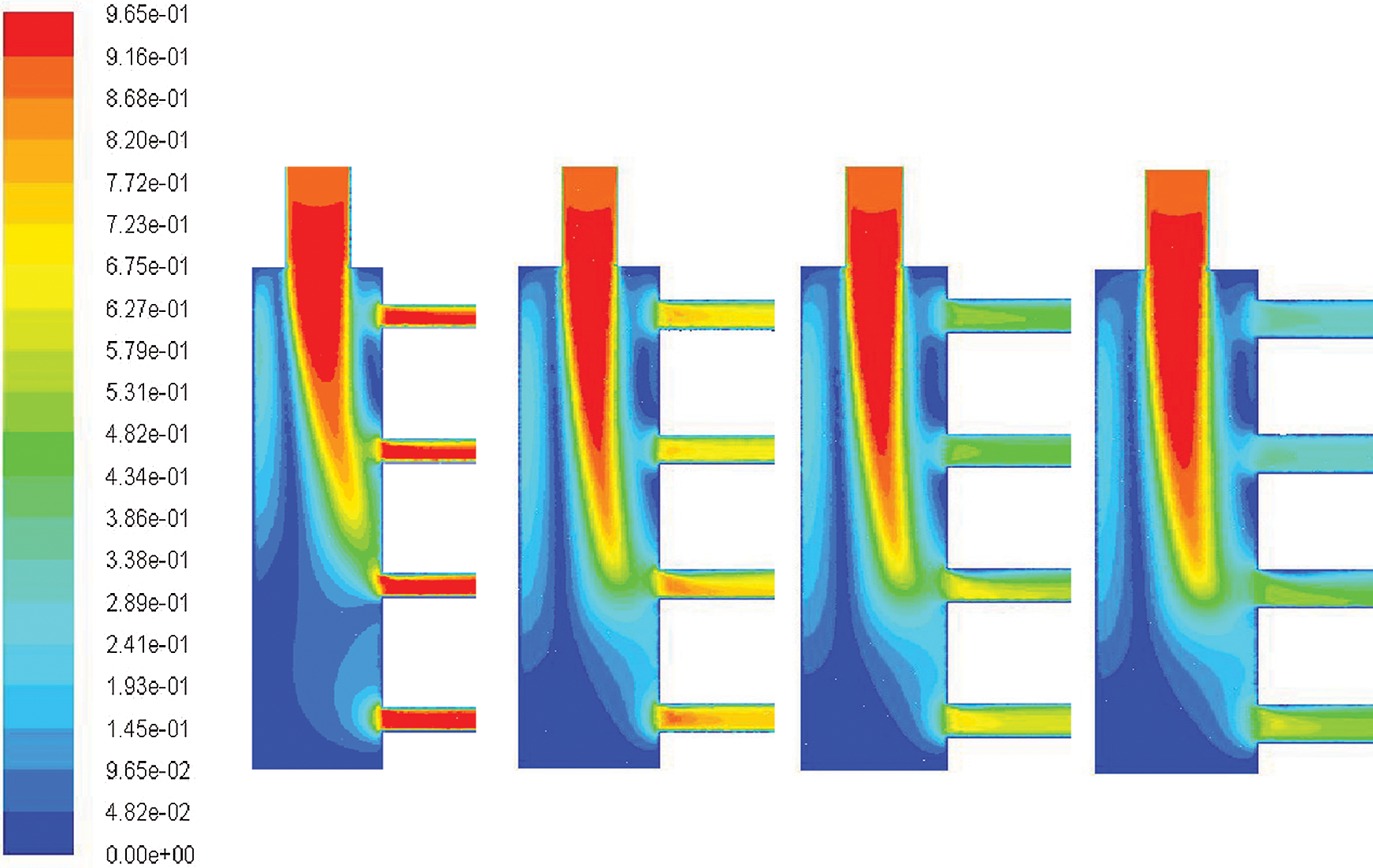
Figure 6: Velocity comparison cloud diagram corresponding to the inner diameters of different outlets when the inner diameter of the shunt chamber was 25 mm
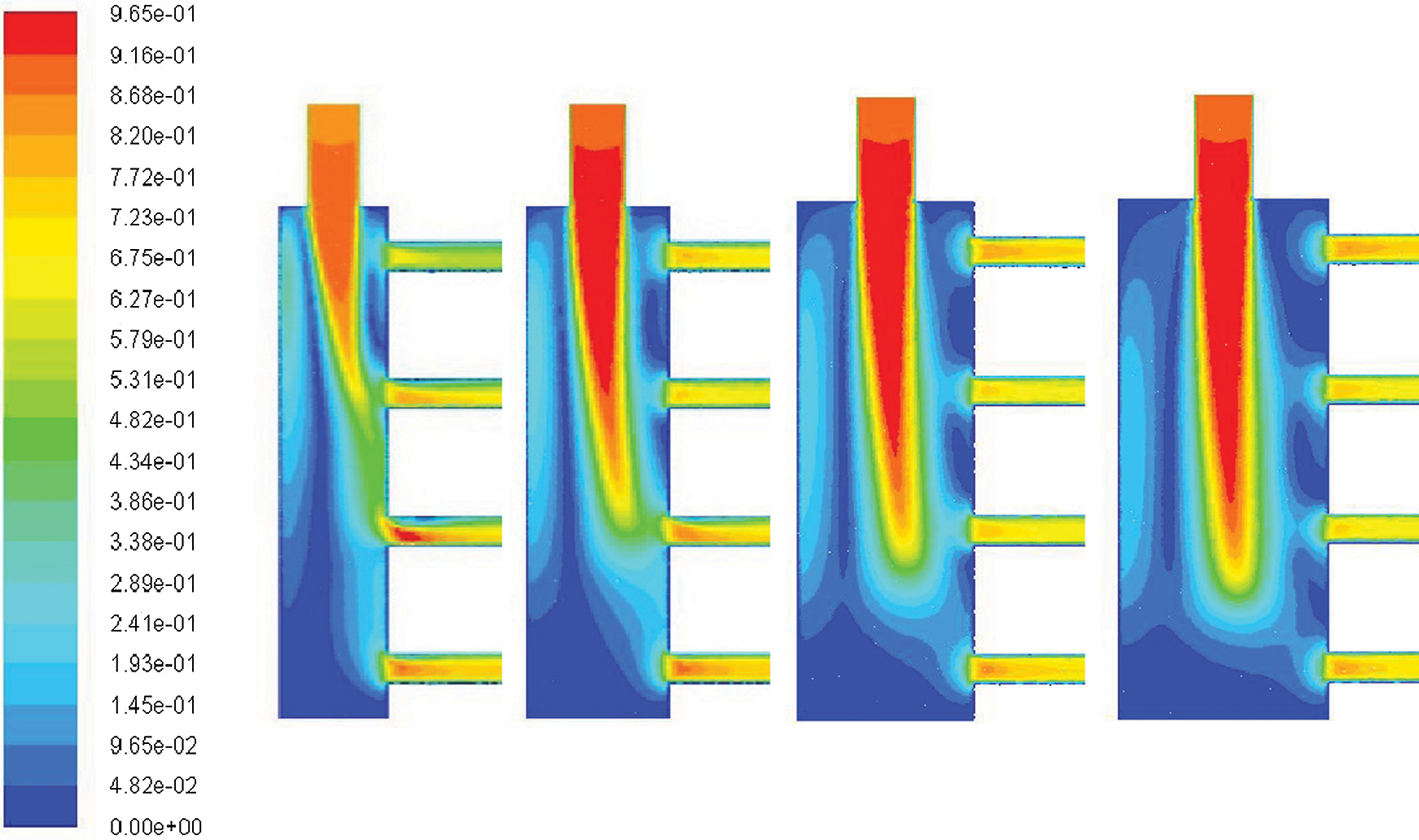
Figure 7: Velocity comparison cloud diagram corresponding to the inner diameter of different shunt chamber when the inner diameter of the outlet is 6 mm
As shown in Fig. 6, when the inner diameter of the water outlet was 5 mm, the outflow speeds of the outlets were approximately identical. The shunt effect was acceptable when the inner diameter of the outlet was 6 mm; however, this effect was poor when the inner diameter of the outlet was 7 or 8 mm.
Thus, assuming that the inner diameter of the shunt chamber is fixed, the shunt effect gradually deteriorates with an increase in the inner diameter of the water outlet, resulting in an increased flow rate at outlet 4 compared with the other outlets. This is denoted as conclusion (1).
Fig. 7 indicates that the flow rates of the outlets were approximately identical when the inner diameter of the shunt chamber was 35 and 30 mm; however, this effect was poor when the shunt chamber was 25 or 20 mm.
Thus, assuming that the inner diameter of the outlet is fixed, the shunt effect gradually improves with an increase in the inner diameter of the shunt chamber, resulting in more homogeneous flow rates among the outlets. This is denoted as conclusion (2).
A statistical analysis considering all 16 models indicated that the flow rate of each outlet was dependent on the inner diameter of the outlet and the inner diameter of the shunt chamber, as shown in Fig. 8.
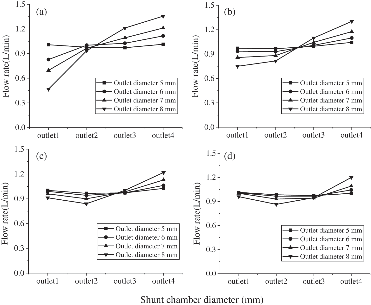
Figure 8: Dependence of the flow rate of each outlet on the inner diameter of the shunt chamber and outlet (a) 20 mm (b) 25 mm (c) 30 mm (d) 35 mm
Conclusion (1) is supported by Fig. 8, as the shunt effect gradually deteriorates owing to the increase in the inner diameter of the water outlet if the inner diameter of the shunt chamber is fixed, resulting in an increased flow rate at outlet 4 compared with the other outlets. In contrast, the shunt effect is enhanced when the inner diameter of the water outlet is reduced.
Conclusion (2) is supported by Fig. 8, as the shunt effect gradually deteriorates if the inner diameter of the shunt chamber increases, assuming that the inner diameter of the water outlet is fixed, resulting in more homogeneous flow rates among the outlets. In contrast, the shunt effect is reduced if the inner diameter of the water shunt chamber is reduced.
To investigate the shunt behavior of the splitter, the following two dimensionless parameters were defined.
1) The structural factor k of the splitter is the ratio of the inner diameter of the water shunt chamber to the inner diameter of the water outlet:
2) The shunt coefficient φi represents the ratio of each outlet flow rate of the splitter to the average value, as follows:
The relationship between k and φi is shown in Fig. 9.
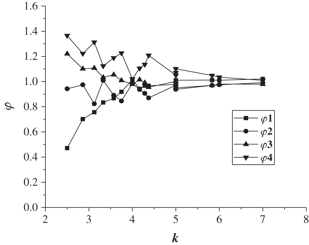
Figure 9: Shunt rules of the splitter
Fig. 9 shows that φi gradually approaches 1 as k increases; therefore, the shunt effect is enhanced when k increases.
However, k should not be excessively large during the design phase, as Dfss increases with k if Dcsk is constant; therefore, the size of the flow splitter may not be reduced. In contrast, if Dfss is constant, Dcsk decreases when k increases, resulting in a greater pressure loss, as shown in Fig. 10.
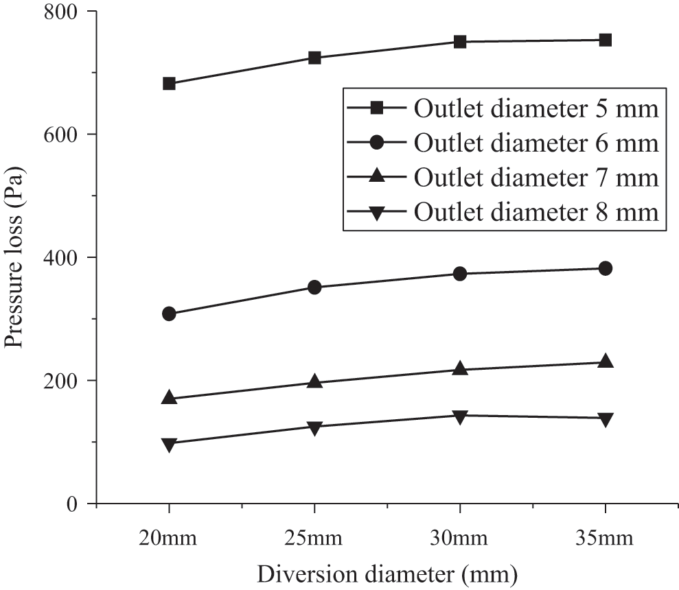
Figure 10: Pressure loss graphs for different models
Consequently, an acceptable flow deviation of each outlet, as well as practical engineering problems, such as miniaturization and excessive pressure loss, should be considered when selecting k. The recommended range of k is 5 ≤ k ≤ 6.
5 Results of Design-Optimization Experiment
5.1 Determination of Optimal Splitter Scheme
In the optimal design of the splitter, the inner diameters of the shunt chamber and outlet were 30 and 6 mm, respectively, considering the shunt effect and pressure loss. The three-dimensional (3D) model and 3D-printed physical model are shown in Fig. 11.
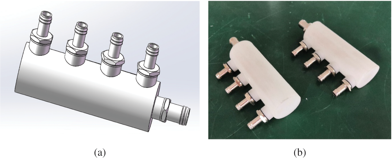
Figure 11: Optimal scheme 3D model and physical model (a) three-dimensional model (b) physical model
5.2 Comparison of Experimental Results between Optimal Splitter and Original Model
Assuming an inlet flow rate of 4 L/min, a flow meter was used to measure the flow rate of each outlet of the optimal design to investigate the shunt effect. A comparison between the experimental results for the optimal and original designs is shown in Fig. 12.
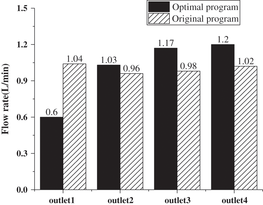
Figure 12: Comparison of experimental results between the optimal and the original scheme
As shown in Fig. 12, the shunt effect in the optimized splitter was significantly improved compared with that in the original design. The deviation of flow rate in each outlet was small in the optimal model, as the minimum and maximum flow rates were 0.96 and 1.04 L/min, respectively, corresponding to a deviation of 8.3% of the minimum value. This deviation was 91.7% lower than the maximum in the original design (100%).
Splitter design experiments and numerical simulations were conducted to validate a simulation method and generate a physical model. Sixteen improved, numerically simulated designs were proposed. According to the dimensionless simulation results, the concept of splitter structural coefficients was proposed, and the optimal splitter design was selected and tested experimentally. The following conclusions are drawn.
1. The shunting effect in the original design was low, and the flow deviation among the outlets was large. The minimum and maximum deviations were 0.6 and 1.2 L/min, respectively, corresponding to a relative deviation of approximately 100% of the minimum flow rate.
2. The main reason for the poor shunt effect in the original splitter is that the inner diameter of the shunt chamber is small and the inner diameter of the outlet is large.
3. For the structural coefficient k, a range of 5 ≤ k ≤ 6 is recommended.
4. In the optimal model, the maximum outlet flow rate is 8.3% higher than the minimum outlet flow rate, corresponding to a significant enhancement of the original design.
Funding Statement: The authors received no specific funding for this study.
Conflicts of Interest: The authors declare that they have no conflicts of interest to report regarding the present study.
1. Azam, M., Xu, T., Khan, M. (2020). Numerical simulation for variable thermal properties and heat source/sink in flow of cross nanofluid over a moving cylinder. International Communications in Heat and Mass Transfer, 118(2), 104832. [Google Scholar]
2. Yang, X. Y. (2018). The advantages and applications of integrated circuits. Science & Technology Innovation and Application, 29, 185–186. [Google Scholar]
3. Cheng, Z. (2018). Discussion on the relationship between artificial intelligence and integrated circuits. Electronic Manufacturing, 2, 67–68. [Google Scholar]
4. Rajaei, H., Dadfar, M. B. (2008). High-performance computing student projects. Computers in Education Journal, 18(1), 79–92. [Google Scholar]
5. Irissou, B., Hughes, J. M., Lanza, L., Kassem, M. K., Wishart, M. S. et al. (2018). Systems for engineering integrated circuit design and development. U.S. Patent 10437953. [Google Scholar]
6. Songkran, W., Chootichai, H., Paisarn, N. (2019). Thermal cooling enhancement of dual processors computer with thermoelectric air cooler module. Case Studies in Thermal Engineering, 14, 100445. [Google Scholar]
7. Song, H. J., Yan, Q., Zhu, X. D. (2017). Design and research on the cooling effect of a computer water cooling system. Research and Exploration in Laboratory, 36(3), 55–58. [Google Scholar]
8. Sun, Y. (2019). Preliminary design study of certain computer water-cooling pump. IOP Conference Series Earth and Environmental Science, 252, 032167. DOI 10.1088/1755-1315/252/3/032167. [Google Scholar] [CrossRef]
9. Birbarah, P., Gebrael, T., Foulkes, T., Stillwell, A., Moore, A. et al. (2020). Water immersion cooling of high power density electronics. International Journal of Heat & Mass Transfer, 147, 118918.1–118918.13. [Google Scholar]
10. Zeng, P., Cheng, G., Liu, J. (2007). Development of single-phased water-cooling radiator for computer chip. Chinese Journal of Mechanical Engineering—English Edition, 20(2), 77–81. DOI 10.3901/CJME.2007.02.077. [Google Scholar] [CrossRef]
11. Xu, P. P., Wu, G., Cao, Y. N., Kong, H. Y. (2012). Research on performance of water cooling plate radiator based on Icepak. Journal of Electronic and Mechanical Engineering, 34(3), 35–39. [Google Scholar]
12. Gao, J. D., Ding, G. L., Hu, H. T., Gao, Q. F., Song, J. (2013). Comparison of shunt performance between diverters of different structures. Refrigeration Technology, 33(3), 24–26+30. [Google Scholar]
13. Azarn, M., Xu, T., Shakoor, A., Khan, M. (2020). Effects of arrhenius activation energy in development of covalent bonding in axisymmetric flow of radiative-cross nanofluid. International Communications in Heat and Mass Transfer, 113, 104547.1–104547.9. [Google Scholar]
14. Azam, M., Mabood, F., Xu, T., Waly, M., Tlili, I. (2020). Entropy optimized radiative heat transportation in axisymmetric flow of Williamson nanofluid with activation energy. Results in Physics, 19(3), 103576. DOI 10.1016/j.rinp.2020.103576. [Google Scholar] [CrossRef]
15. Azam, M., Shakoor, A., Rasool, H. F., Khan, M. (2019). Numerical simulation for solar energy aspects on unsteady convective flow of MHD cross nanofluid: A revised approach. International Journal of Heat and Mass Transfer, 131, 495–505. DOI 10.1016/j.ijheatmasstransfer.2018.11.022. [Google Scholar] [CrossRef]
16. Sahini, M., Kshirsagar, C., Kumar, M., Agonafer, D., Fernandes, J. et al. (2017). Rack-level study of hybrid cooled servers using warm water cooling for distributed vs. centralized pumping systems. 33rd Thermal Measurement, Modeling & Management Symposium (SEMI-THERM), pp. 155–162. IEEE. [Google Scholar]
17. Prasad, P. G., Chilamkurti, P. L., Santarao, K. (2020). Investigation to enhance the performance of computer processor cooling system. IOP Conference Series: Materials Science and Engineering, 954(1), 012022. DOI 10.1088/1757-899X/954/1/012022. [Google Scholar] [CrossRef]
18. Liu, S., Huang, G. (2021). High-density block transformation to increase natural ventilation based on CFD simulation. Fluid Dynamics and Materials Processing, 17(1), 141–157. DOI 10.32604/fdmp.2021.011990. [Google Scholar] [CrossRef]
19. Anilkumar, G., Krishna, G. R., Kumar, G., Palanisamy, K. (2020). Performance analysis of solar updraft tower using Ansys fluent. IOP Conference Series: Materials Science and Engineering, 937(1), 012022. DOI 10.1088/1757-899X/937/1/012022. [Google Scholar] [CrossRef]
20. Wang, F. J. (2004). Computational fluid dynamics analysis. Peking: Tsinghua University Press. [Google Scholar]
21. Wang, S. I. (2011). Advanced engineering fluid mechanics. Peking: China Electric Power Press. [Google Scholar]
22. Zhu, H. J., Lin, Y. H., Xie, L. H. (2011). FLUENT 12 fluid analysis and project simulation. Peking: Tsinghua University Press. [Google Scholar]
23. Khawaja, H., Moatamedi, M. (2018). Semi-implicit method for pressure-linked equations (simple) solution in Matlab. International Journal of Multiphysics, 12(4), 313. [Google Scholar]
24. Kozelkov, A. S., Lashkin, S. V. (2020). An efficient parallel implementation of the SIMPLE algorithm based on a multigrid method. Numerical Analysis and Applications, 13(1), 1–16. DOI 10.1134/S1995423920010012. [Google Scholar] [CrossRef]
 | This work is licensed under a Creative Commons Attribution 4.0 International License, which permits unrestricted use, distribution, and reproduction in any medium, provided the original work is properly cited. |