Materials Processing
| Fluid Dynamics & Materials Processing |
DOI: 10.32604/fdmp.2021.015422
ARTICLE
Mixed Convection in a Two-Sided Lid-Driven Square Cavity Filled with Different Types of Nanoparticles: A Comparative Study Assuming Nanoparticles with Different Shapes
1Laboratory of Mechanics, Faculty of Sciences Aïn-Chock, University Hassan II, Casablanca, Morocco
2Department of Mechanical Engineering, Royal Air School, Marrakech, 40002, Morocco
3Department of Physics, Faculty of Sciences, University 20 August 1955, Skikda, 21000, Algeria
*Corresponding Author: Mehdi Riahi. Email: mehdi_riahi@hotmail.fr
Received: 17 December 2020; Accepted: 01 March 2021
Abstract: Steady, laminar mixed convection inside a lid-driven square cavity filled with nanofluid is investigated numerically. We consider the case where the right and left walls are moving downwards and upwards respectively and maintained at different temperatures while the other two horizontal ones are kept adiabatic and impermeable. The set of nonlinear coupled governing mass, momentum, and energy equations are solved using an extensively validated and a highly accurate finite difference method of fourth-order. Comparisons with previously conducted investigations on special configurations are performed and show an excellent agreement. Meanwhile, attention is focused on the heat transfer enhancement when different nano-particles: Cu, Ag, Al2O3, TiO2 and Fe3O4 are incorporated separately in different base fluids such as: Water, Ethylene-glycol, Methanol and Kerosene oil. In this framework, the numerical results related to several mixtures are presented and concern flow pattern and heat transfer curves for various values of Richardson number [Ri = 0.1, 1 and 10]. It turns out that the choice of the efficient binary mixture for an optimal heat transfer depends not only on the thermophysical properties of the nanofluids but also on the range of the Richardson number. Special attention is devoted to shedding light on the effect of the shape of the nanoparticles on the heat transfer in the case of Water-Ag nanofluid. It is concluded that the spherical shape is more suitable for a better heat transfer enhancement in comparison to the cylindrical ones.
Keywords: Nanofluids; mixed convection; lid-driven square cavity; numerical simulation
List of symbols:
| | Specific heat |
| | Average molecular diameter of the water |
| | Nanoparticles diameter size |
| | Gravity acceleration |
| | Grashof number |
| | Thermal conductivity |
| | Boltzmann constant |
| | Cavity length |
| | Pressure |
| | Modified Pressure |
| | Prandtl number |
| | Brownian-motion Reynolds number |
| | Reynolds number |
| | Richardson number |
| | Time |
| | Temperature |
| | Cold-wall temeprature |
| | Hot-wall temperature |
| | Freezing temperature of water-based fluid |
| | Cartesian coordinates |
| | Velocity components |
| | Characteristic velocity |
| Greek symbols: | |
| | Thermal expansion coefficient |
| | Dynamic viscosity |
| | Density |
| | Heat capacitance |
| | Nanoparticles volume fraction |
| | Dimensional variable |
| | Dimensionless variable |
| Subscripts: | |
| | Cold |
| | Fluid |
| | Hot |
| | Nanofluid |
| | Nanoparticles |
| | Relative thermophysical properties |
Fluid flow and mixed-convection heat transfer in nanofluid-filled enclosures represent a complicated flow phenomenon due to wall motion that involves forced convection and temperature difference that causes natural convection induced by buoyancy. This kind of flow is of great interest in many industrial sectors, such as the industrial cooling systems applied either for heating or cooling, solar collectors, chemical processing equipment, float glass production, drying technologies, etc. Conventional heat transfer fluids such as water and ethylene glycol, with their low thermal conductivity, limit the performance and compactness of many industrial and engineering electronic devices. Nanofluids are the ideal solution for these equipments since the thermal conductivity of the nanoparticles projected in suspension in the conventional fluid, improves the heat transfer. Different nature of nanoparticles are concerned by this topic including metals (Al, Cu), oxides (Al2O3, TiO2, and CuO), carbides (SiC), nitrides (AlN, SiN) or nonmetals (Graphite, carbon nanotubes) while the base fluid is usually a conductive fluid, such as water, ethylene glycol or methanol depending on application field.
Tiwari et al. [1] investigated numerically the heat transfer enhancement in mixed convection between two-sided lid-driven differentially heated square cavity utilizing nanofluids. The nanofluid used by these authors was Copper-Water nanofluid having Prandlt number Pr = 6.2 and solid volume fraction χ varied up 12%. The upper and the bottom walls are considered thermally insulated while the left and the right moving walls are maintained at different constant temperatures. It was found that the pattern formation and the heat transfer in the cavity can be greatly influenced by both the Richardson number and the direction of the moving walls.
Several studies have been interested by the same purpose in the literatures [2–5]. For instance, Rana et al. [2] have numerically studied the heat transfer enhancement in steady mixed convection flow along a vertical plate with heat source/sink utilizing nanofluids. They emphasized the effect of spherical and cylindrical shaped nanoparticles on the heat transfer using different water-based nanofluids containing Cu, Ag, CuO, Al2O3, and TiO2. It was proved that the use of nanotubes (cylindrical shaped nanoparticles) have higher heat transfer enhancement as compared to spherical shaped nanoparticles. Also, it was shown that Ag nanoparticles proved to have the highest cooling performance for this vertical plate problem where TiO2 nanoparticles have the lowest. These results have been attributed according to these authors to the high thermal conductivity of Ag and the low thermal conductivity of TiO2.
In the same framework but in the natural convection, Zaraki et al. [6] have performed a theoretical analysis of boundary layer heat and mass transfer of nanofluids with emphasis on the effects of size, shape and type of nanoparticles, type of base fluid and working temperature. The model adopted in their analysis takes into account the effects of Brownian motion and thermophoresis. It was concluded that the choice of material types of nanoparticles was crucial. Indeed, for some type of nanoparticles significant enhancement of the heat transfer rate was observed, while some others can significantly deteriorate the heat transfer from the surface. For example, the dispersion of 40 nm spherical zinc-oxide nanoparticles in water enhances the heat transfer while dispersion of 43 nm of spherical alumina nanoparticles in water leads to a deterioration of the heat transfer [6].
Raza et al. [7] have developed a house code to study the effect of different base fluids on the hydrodynamic and thermal characteristics of Titania nanofluids in cylindrical annulus with discrete heat source. He found that the impact of TiO2 nanofluid heat transfer is related to the basic fluid types.
In this paper, we extend the analysis performed by Tiwari and Das to investigating the heat transfer in this system when different types and shapes of nanoparticles are incorporated in different base fluids. We consider the case where the right wall moves down while the left wall moves to the top which represents the case where the shear and the buoyancy forces act in opposite directions. Using highly validated Fourth-order compact numerical method for the resolution of the nonlinear equations governing the complex physics of the system, we attempt to shed light on the effect of the nature and the shape of the nanoparticles dispersed in different types of base fluids on the heat transfer enhancement in the cavity.
This paper is organized as follows: The studied configuration and its related mathematical formulation are defined in Section 2. Section 3 is devoted to presenting details of the numerical formulation used to solve the heat transfer problem and comparison with the existing results in specific configurations. In Section 4, pertinent results are discussed while the conclusion is addressed in Section 5.
The geometry of the present problem is shown in Fig. 1. It consists of a two-dimensional square cavity with the height of L. The temperature of the right wall is considered to be maintained at high temperature of Th as the left sidewall is kept at low temperature of Tc. The horizontal walls are adiabatic and impermeable. The vertical walls are moving with the same velocities in different directions such as the right wall moves downwards with the constant velocity Vp while the left one moves upwards with –Vp. The cavity is filled with a nanofluid with different nanoparticles immersed separately in different base fluids where their pertinent thermophysical properties are given in Tabs. 1 and 2.
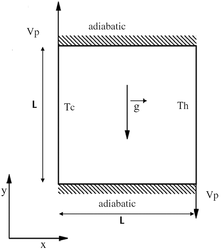
Figure 1: Configuration of the problem in the case of the mixed convection
Table 1: Thermophysical properties of nanoparticles
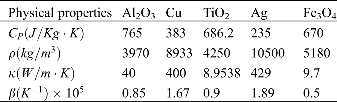
Table 2: Thermophysical properties of base fluids
The flow is considered incompressible, steady and laminar and governed by the laws of conservation of mass, momentum and energy. Taking into account these assumptions, these equations take the following form:
The density
where
In order to proceed to the numerical solution of the system Eqs. (1)–(4) the following dimensionless variables are introduced:
By substitution of Eqs. (5) into Eqs. (1)–(4), the following system of equation is derived:
The dimensionless parameters appeared in the problem under consideration are:
and the boundary conditions are:
To go from the pressure-velocity formulation (u, v, p) to the stream function-vorticity formulation (ψ, ω) where
the system of equations governing the dynamics of the physical problem is written in the following general form
where
For the first and second x-derivatives, the following discretizations with fourth order precision are considered:
where
Substituting the expressions (18) and (19) and their corresponding
while the general conservation equation becomes:
Considering the obtained form of the Eq. (20), one can remark that the fourth
And by using the standard form of second-order centered discretization, the Eqs. (22) and (23) can be written as:
Taking into account these expressions, we obtain finally the following finite difference form of the kinematic equation:
whose solution is a solution of the stream function Eq. (16) with a fourth-order spatial precision.
The same approach is applied to obtain the fourth-order approximation of the general conservation equations along the (
The final form of our fourth order compact formulation (FOCF) scheme of the equations governing the dynamics of the system is as follows:
with:
where
And
Note that if A, B, C, D, E and F vanishes, the Eqs. (29) and (30) are reduced to the second order formulation. These equations associated to the boundary conditions are solved numerically by the implicit scheme with alternating directions (ADI: Alternating directions Implicit) method established by Peaceman et al. [9] in 1955 which consists in advancing half a step of time following
Such iterative numerical algorithm requires pseudo time derivatives to be assigned to the equations presenting the physical system such as:
The solution of this system will not depend on the time derivative introduced by the numerical scheme since we are dealing with a steady flow configuration where the source of unsteadiness does not exist. Consequently, a first order (Δt) accurate which is an implicit Euler step is added to these pseudo time derivatives as well as to the non-linear terms in the general conservation equation. In this framework, the system of Eqs. (32) and (33) is rewritten as follows:
This approach has been used recently by Erturk et al. [10] where the solution of the Eqs. (34) and (35) converge always toward that of the steady Eqs. (16) and (17). For avoiding any kind of repetition in this paper, we will not present the different steps used by these authors and the reader should be referred to [10] for more details.
In order to check the convergence of the obtained results during the iterations, several residuals factors are calculated. We define the first residual expression related to the stream function and the general conservation function respectively as follows:
The value of RES1 is an indication related to the time derivatives introduced by the numerical procedure. It would generally vanish since the solution converges to the steady state.
A second residual parameter, RES2, is defined by the following expressions presenting the difference in absolute value between two successive iteration steps for the variables stream function, vorticity and energy:
RES2 gives an indication of the significant digit on which the code is iterated.
The third residual parameter, RES3, is similar to RES2 except that it is normalized by the representative value of the previous time step. This makes possible to get an indication later on the maximum percentage variation of change in ψ and Γ at each iteration step. RES3 is defined as follows:
In our calculations and for all Rayleigh numbers, we consider that convergence is obtained when both
3.1 Boundary Condition for the Vorticity
Dimensionless boundary conditions for ψ are:
For vorticity, Störtkuh et al. [11] have presented an analytical asymptotic solution near the corners of cavity and using finite element bilinear shape functions and they also have presented a singularity-removed boundary condition for vorticity at the corner points as well as at the wall points.
In this study, we follow Störtkuh et al. [11] for the boundary conditions and use the following expressions for calculating vorticity values at the walls:
and at the corner points:
where V is the velocity of the walls. In our case, this velocity equals 1 for the left vertical wall, –1 for the right vertical wall whereas 0 for the other horizontal walls.
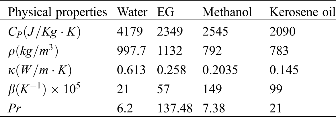
In explicit notation, for the wall points shown in Fig. 2a, the vorticity is calculated as following:
Figure 2: Grid points at the walls and at the corners: (a) wall points and (b) corner points
Similarly, for the corner points shown in Fig. 2b, the vorticity is calculated as the following:
The reader should be referred to Störtkuh et al. [11] for more details on the boundary conditions.
The averaged and the local heat transfer rates at the left cold wall of the cavity are presented in terms of the averaged Nusselt numbers,
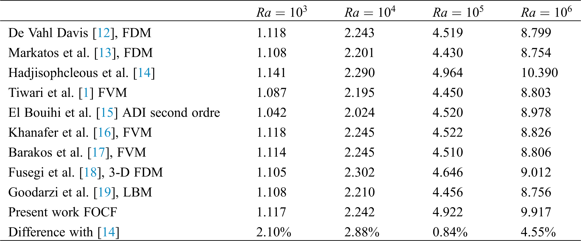
A good concordance is found by comparing the results obtained by our numerical code with those of de Vahl Davis [12], Markatos et al. [13], Hadjisophcleous et al. [14], Tiwari et al. [1], El Bouihi et al. [15], Khanafer et al. [16], Barakos et al. [17], Fusegi et al. [18] and Goodarzi et al. [19]. This comparison is performed on the problem of natural convection in a differentially heated square enclosure filled with air having the Prandlt number Pr = 0.71. In Tab. 3, we report the numerical values of the average Nusselt number obtained for different values of the Rayleigh number.
Table 3: Average Nusselt number comparison with previous works
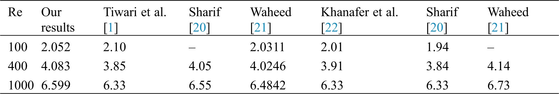
For giving more reliability to our code, we attempt to compare our numerical results with previous works concerned by mixed convection in differentially heated cavity containing air where the top wall is moving with a constant velocity and kept hot while the bottom wall is cooled. The two vertical walls are insulated. At Gr =⟬
Table 4: Comparison of the Nusselt number with previous works (C.V.M)
Computations with reasonable accuracy require an optimum choose of the mesh. For that, we start by shedding light on the influence of the size and nodes distribution on the average Nusselt number
Table 5: Values of the physical quantities and for different grid values
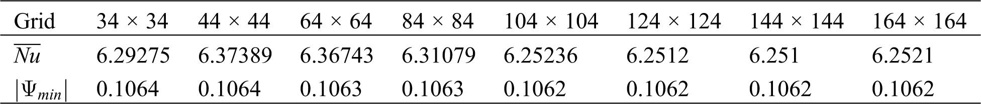
This grid test is performed on the framework of a mixed convection configuration using square cavity filled with air (Pr = 0.71) with a vertical thermal gradient and moving upper horizontal wall.
4.2 Heat Transfer and Pattern Formation in Ag-Water Nanofluid
Our attention is focused on the mixed convective regimes where both forced and natural convections coexist corresponding to a Richardson number range
The configuration we considered in this study is when the left vertical wall moves constantly upward while the right one moves downwards with the same velocity. Here, the buoyancy and shear forces are opposing each other. The Grashof number is fixed at
Fig. 3 illustrates the streamlines (left part) and the isotherms (right part) for Water and Water-Ag nanofluid when gradually increasing the volume fraction (χ = 0.04, 0.2) when Ri = 0.1. As one can see from the Figs. 3a–3c and 3e–3g, the flow pattern is not influenced by the presence of the nanoparticles where only one convective roll is formed in the whole cavity. The direction of rotation of this cell is clockwise as it can be deduced from the vertical velocity profile related to this case plotted at the mid-plane
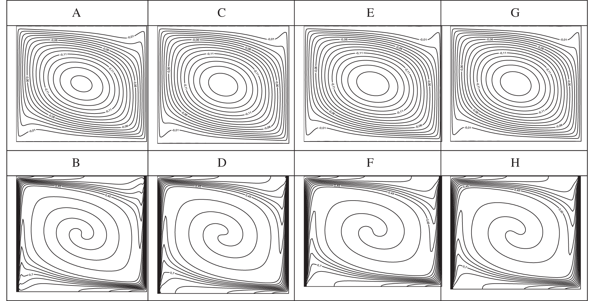
Figure 3: Streamlines (A, C, E, G) and isotherms (B, D, F, H) for
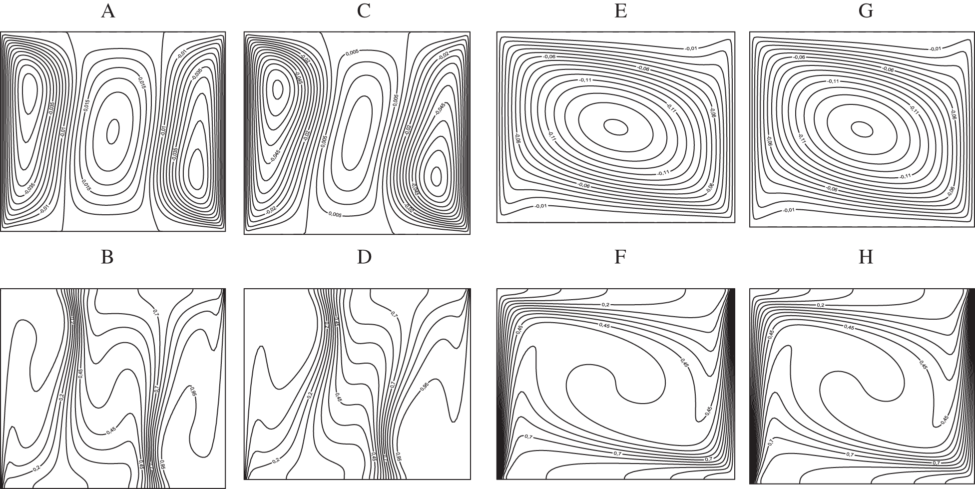
Figure 4: Streamlines (A, C, E, G) and isotherms (B, D, F, H) for
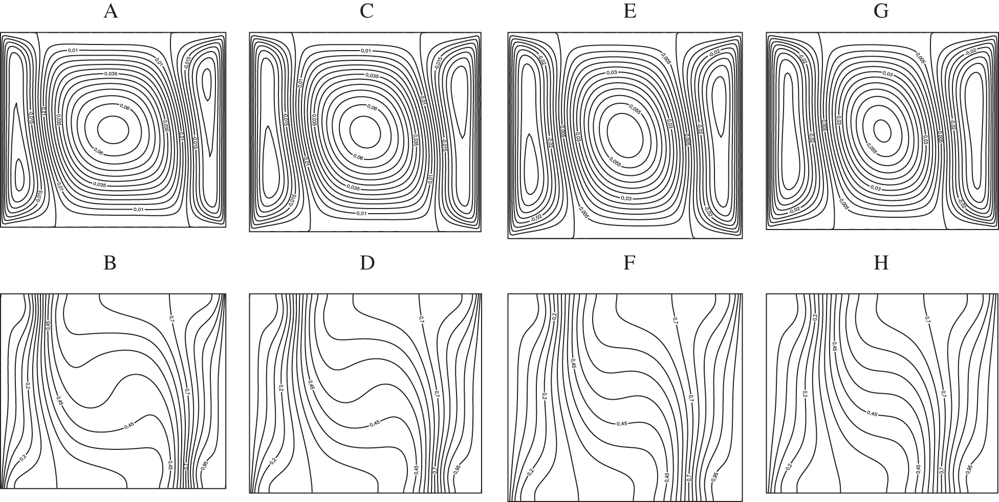
Figure 5: Streamlines (A, C, E, G) and isotherms (B, D, F, H) for
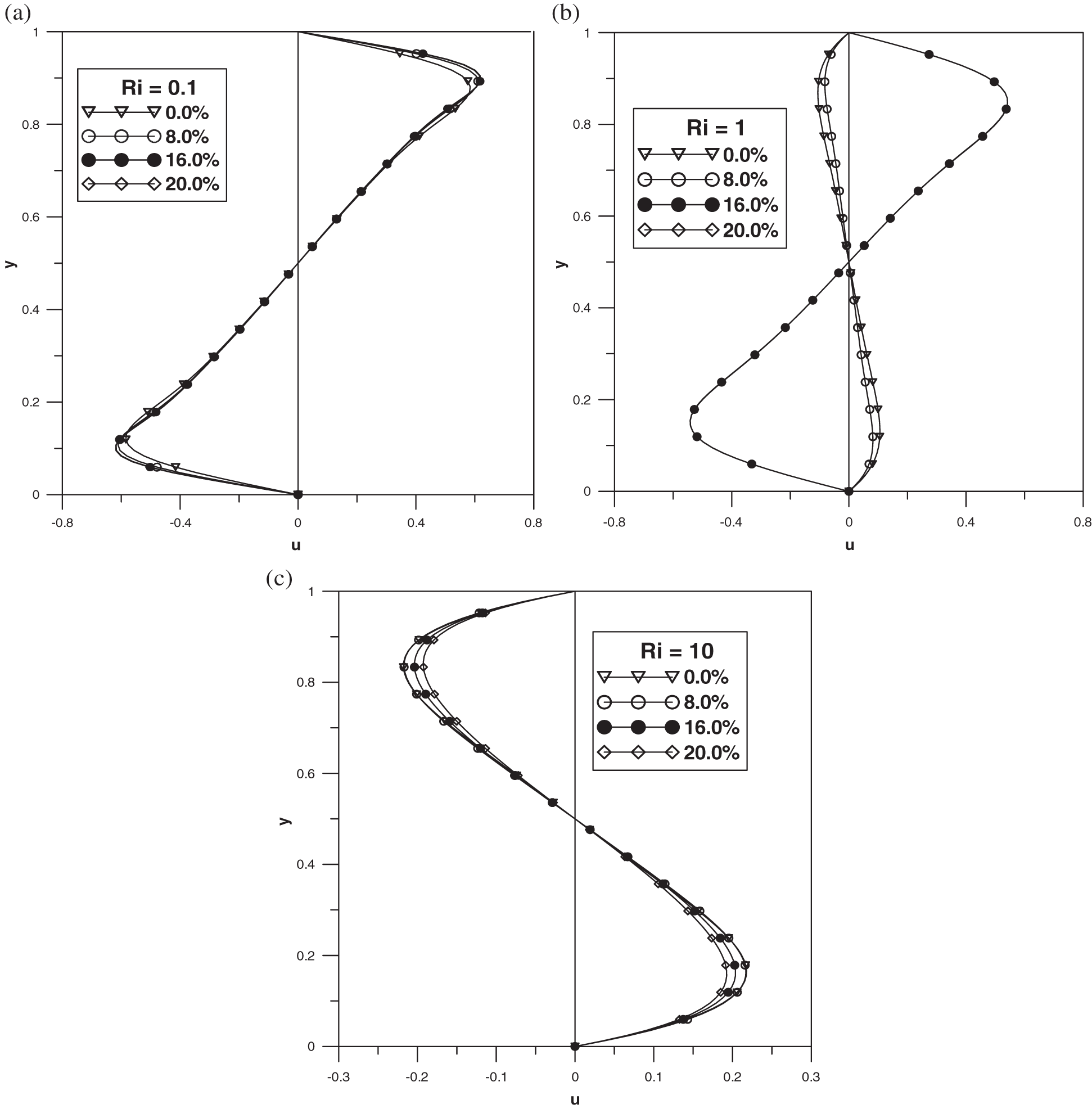
Figure 6: Vertical mid-plane u-velocity: (a)
This symmetry property means that the flow, at this mid-plan, changes its direction from the upper half of the cavity
The isotherms related to this configuration are depicted in Figs. 3b–3d and 3f–3h where a strong convection is noticed for all the values of the nanoparticle fractions. Similarly to the streamlines, the isotherms are present in the left-upper and right-lower corners ensuring heat transfer in these regions. The temperature at the horizontal mid-plane
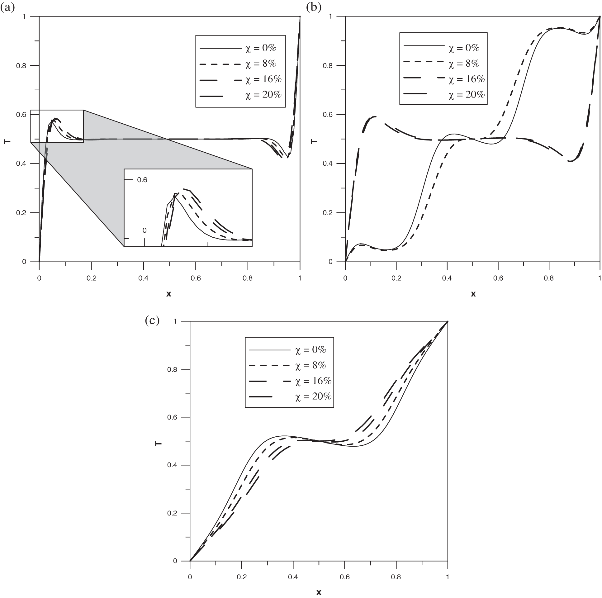
Figure 7: Horizontal mid-plane temperature profile: (a)
The interval
Decreasing the Reynolds number until Ri =1 is reached, the flow pattern and the heat transfer characteristics are changed as shown in Fig. 4. Indeed, secondary flow composed by three cells is observed for
Regarding the isotherms, two thermal boundary layers are formed when
The case where natural convection becomes much more important than forced convection corresponds to Ri = 10. Here, as it was mentioned by Tiwari et al. [1] it is expected that the nanoparticles do not affect neither the fluid dynamics nor the heat transfer since their brownian motion is not taken into account in the model. This feature can be clearly seen from Fig. 5 related to the streamlines and the isotherms. In fact, the flow structure is composed by three cells similarly to the case where the natural and the forced convections are with the same order of magnitude, Ri = 1, with weak amount of nanoparticles. One can also observe the same velocity profiles at the mid-plane
We will now discuss the heat transfer in our system by referring to the local Nusselt number Nu at the cold wall located at the left side of the cavity. Fig. 8 displays the evolution of Nu for different values of
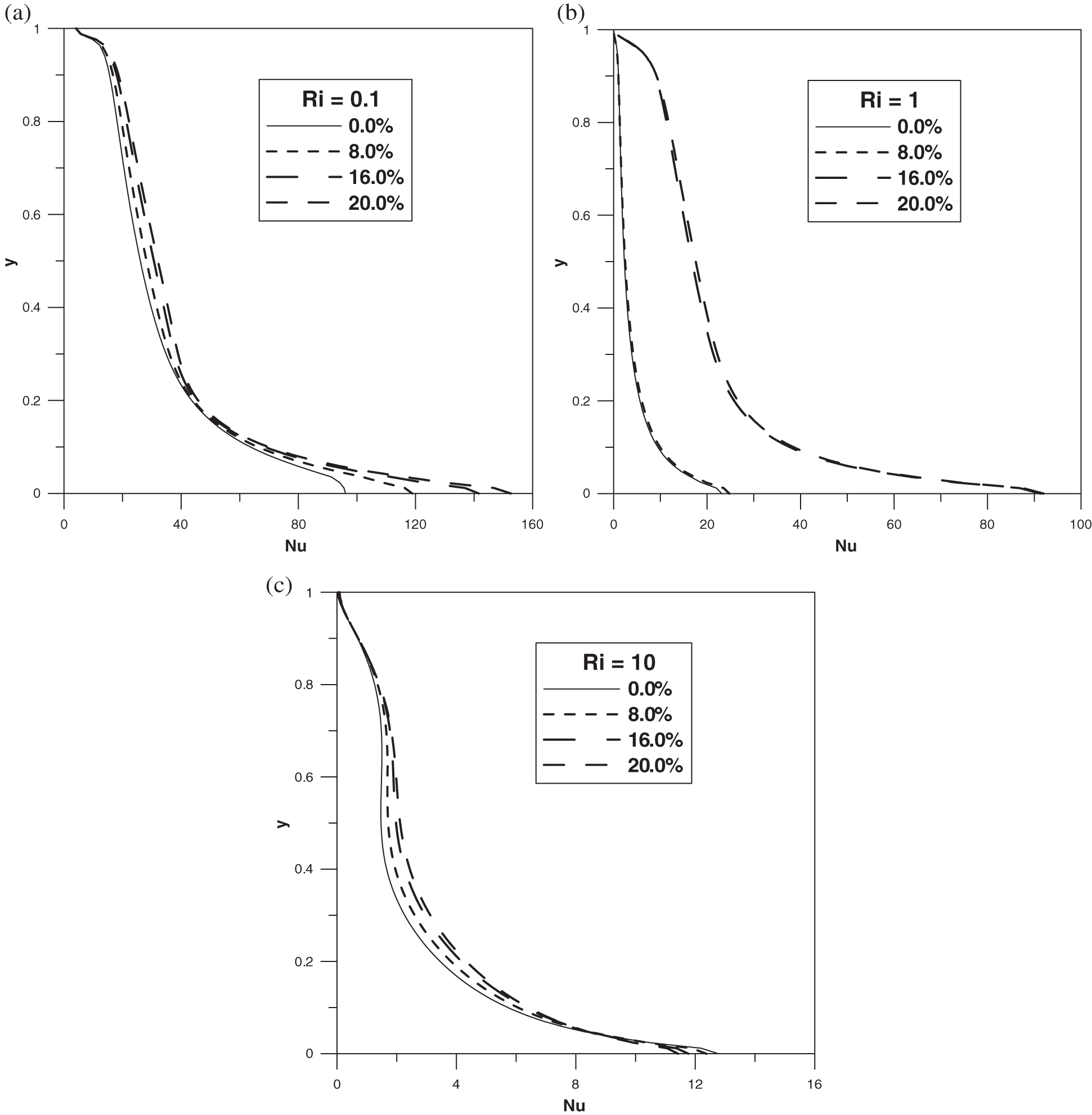
Figure 8: Local Nusselt number at the left wall: (a)
4.3 Effect of the Nanoparticles Type
In this subsection, we shall concentrate our attention on highlighting the effect of the type of nanoparticles on the pattern formation as well as in the heat transfer into the cavity. For that, five types of nanoparticles are taken into consideration such as: Ag, Cu, TiO2, Fe3O4 and Al2O3. The obtained results in this framework show that the fluid dynamics is not influenced by changing the type of the nanoparticles in the sense that we obtain the same streamlines and isotherms discussed above for the Ag nanoparticles. We will not here present these results for avoiding any kind of repetition in the paper. However, the type of nanoparticles affects the heat transfer in the cavity as shown in Fig. 9 where evolution of the average Nusselt number versus the volume fraction is displayed for the five types of nanoparticles and for the different values of Richardson. As one can see, we recover the classical observation claiming that the presence of nanoparticles enhances the heat transfer in the cavity in comparison to the pure base fluid independently on whether the natural convection is more or less dominant in comparison to the forced convection. This effect depends on the nature of the nanoparticles and becomes more pronounced in the high values of the volume fraction. Indeed, the parameter
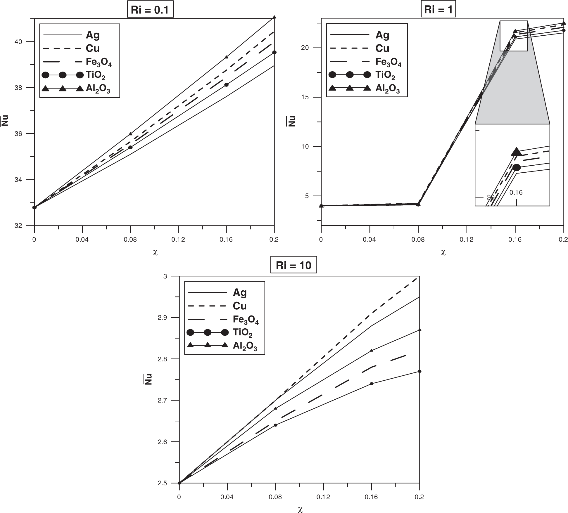
Figure 9: Average Nusselt number versus the volume fraction of the nanoparticles for different values of Richardson number
These features can be explained of the basis of the thermophysical properties of each substance and there implications depending on the mechanism driving the flow. Indeed, when Ri = 10 the flow is driven by natural convection and consequently the thermal properties of the nanoparticles especially the thermal conductivity, thermal expansion coefficient and heat capacity play a significant role and mainly contribute in the flow dynamics as well as in the heat transfer in comparison to the hydrodynamical quantities such as the dynamic viscosity and the mixture’s density. However, in the case of weak values of Ri the flow is driven mainly by the walls velocities and hence the hydrodynamic quantities are more involved than the thermal ones. In addition, the thermal behavior obtained in this study confirm that the nanofluids heat transfer depends not only on the thermal conductivity of the nanoparticles and the dynamic viscosity of the nanofluid as suggested by several studies in the literature but it depends on a combination of all the thermophysical properties of these substances. To confirm this statement, one can observe from the Tabs. 1 and 2 that
while for the average Nusselt number none of these orders is conserved.
One the other hand, the local Nusselt number at the left cold wall varies versus the vertical coordinate with the same shape meaning that it always decreases versus y. Also, this transfer parameter is not remarkably influenced by the type of the nanoparticles as shown in Fig. 10 at the volume fraction
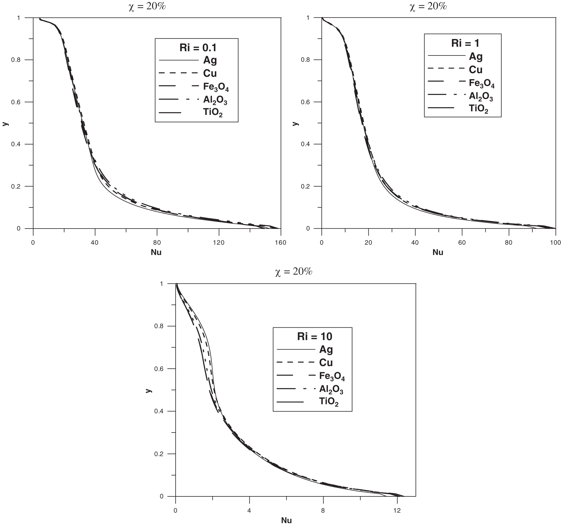
Figure 10: Local Nusselt number at the left wall: (a)
To conclude, the effect of the nature of the nanoparticles on the enhancement of the heat transfer observed in this system cannot be understood on the basis of the present study. However, one can confirm that this is a phenomenon that cannot be solely attributed to the higher thermal properties of the added nanoparticles especially when both natural and forced convection regimes are involved in the system. Consequently, much effort has to be deployed in this direction for a better understanding of the mechanism controlling the heat transfer in systems with nanofluids.
4.4 Heat Transfer and Pattern Formation in Ag-Ethylene-Glycol Nanofluid
Do the heat transfer and the fluid dynamics change when the water is substituted by Ethylene-glycol in this studied configuration? This is the question that we attempt to address in this subsection. For that we consider a nanofluid with Ag-Ethylene-glycol mixture. Streamlines and isotherms related to this solution is depicted in Figs. 11–13 for three different values of Richardson number, Ri = 0.1, 1, 10.
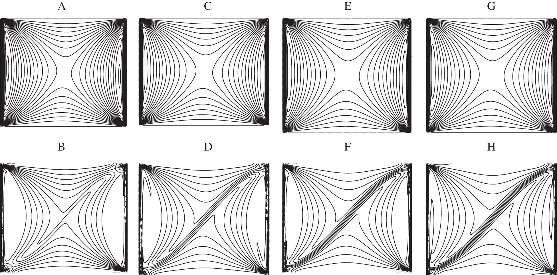
Figure 11: Streamlines (A, C, E, G) and isotherms (B, D, F, H) for
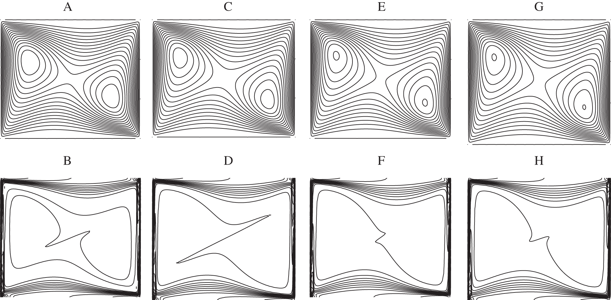
Figure 12: Streamlines (A, C, E, G) and isotherms (B, D, F, H) for
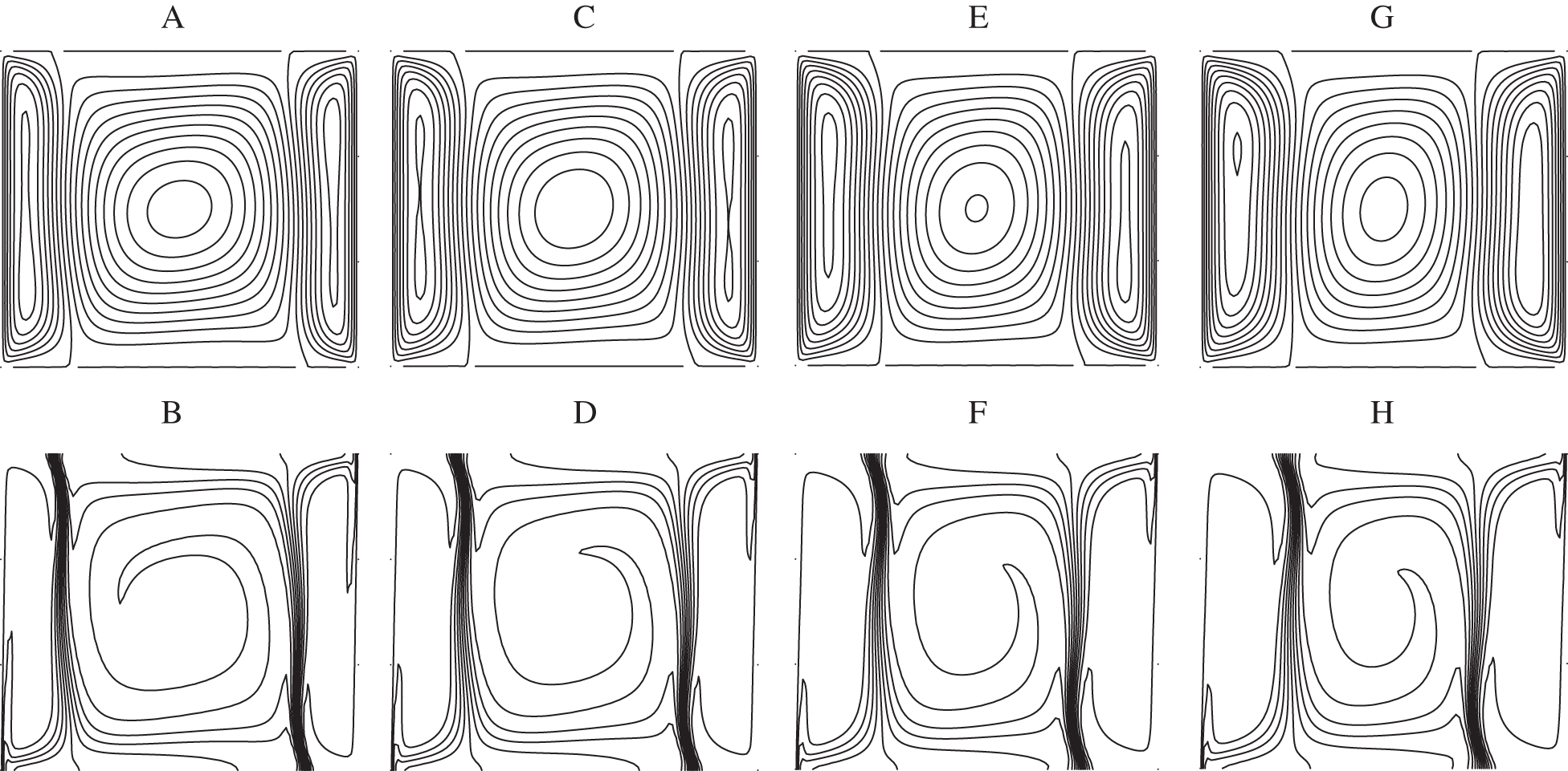
Figure 13: Streamlines (A, C, E, G) and isotherms (B, D, F, H) for
As one can see from Figs. 11a–11c and 11e–11g), when Ri = 0.1 weak vortices are appeared next to the moving walls whereas next to the horizontal upper/lower walls the streamlines exhibit minimums/maximums that become more accentuated when approaching towards the center of the cavity. The same behavior is observed for the isotherms as depicted in Figs. 11b–11d and 11f–11h. One can also look at the corners of the cavity that show a particular behavior in comparison to the Ag-Water nanofluid. Indeed, the four corners of the cavity are occupied by the nanofluid in contrast to the case of water based nanofluid where only the left-upper and right-lower corners that are occupied by the nanofluid. Therefore, the Ethylene-glycol ensures a good distribution of the velocity and the temperature as well as the heat transfer in the cavity in comparison to water. One should also shed light on the formation of a thermal boundary layer in a diagonal direction of the cavity which becomes more pronounced by increasing the nanoparticles volume fraction. This result confirms the increase in the strength of the convection under the effect of the nanoparticles. At Ri = 1 where the buoyancy and the shear forces are of the same order of magnitude, different streamlines and isotherms are obtained in comparison to Ag-water nanofluid as displayed in Fig. 12. In this case, the streamlines are characterized by a large central main eddy, occupying the whole of the cavity, breaking into two small ones at the core. This feature remains unchanged by increasing the volume fraction. In addition and regarding the isotherms, thermal boundary layer is spread out over the four walls of the cavity.
By crossing Ri = 10, the flow is characterized by three vortices similarly to the case of Ag-water nanofluid as shown in Fig. 13. The unique difference that should be noticed here is the thickness of the boundary layer formed at the junction of two counter rotating vortices that becomes thinner in comparaison to the case of Ag-water nanofluid. This results reveals the strength of the convection and the heat transfer in the cavity when the used base fluid is the Ethylene-glycol instead of water. The fluid velocity in the
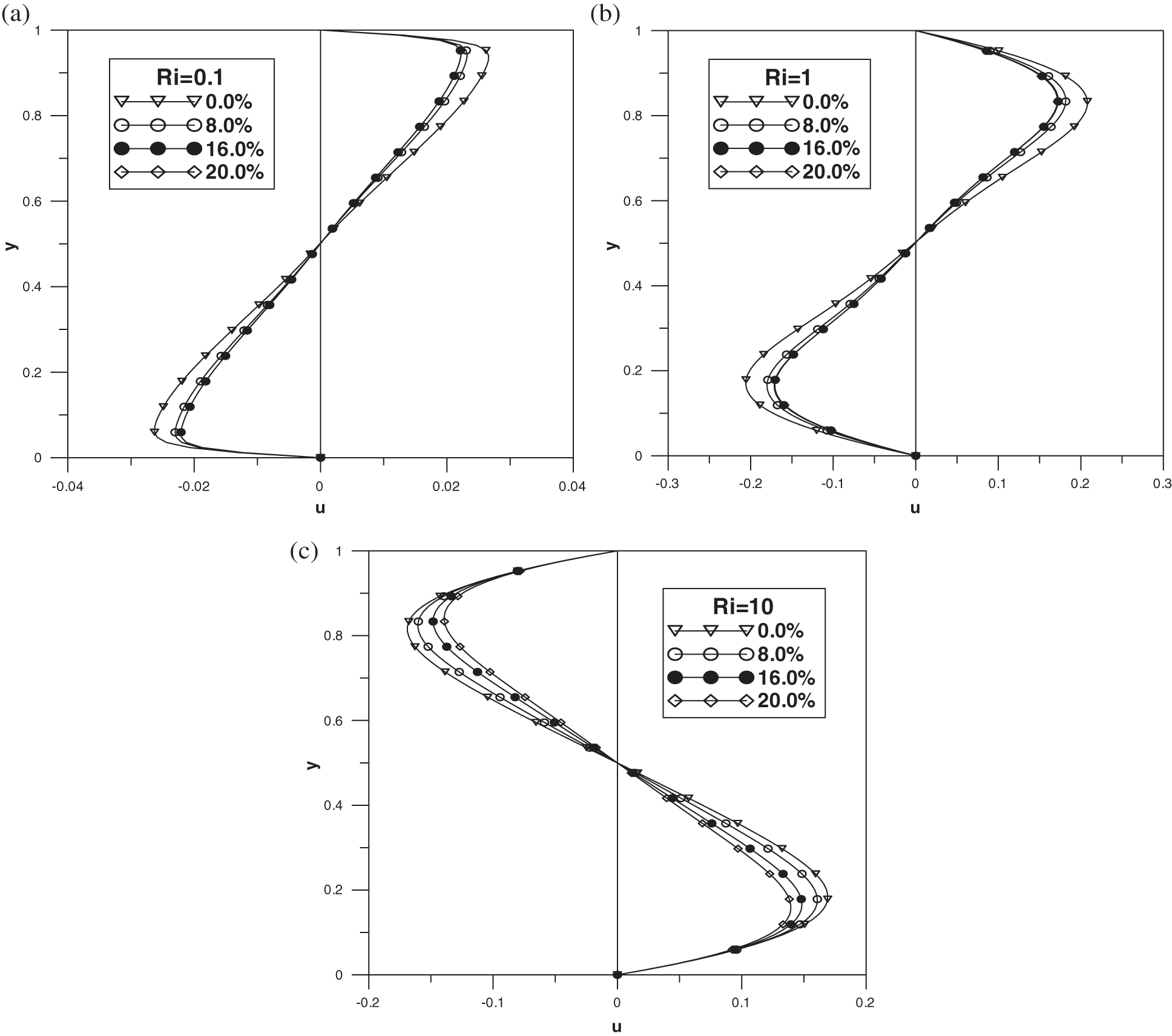
Figure 14: Vertical mid-plane u-velocity: (a)
The shape of this kinematic quantity is symmetric similarly to the Ag-Water nanofluid verifying the Eq. (50). In addition, it is not influenced by the nature of the base fluid in the case Ri = 0.1 except a remarkable change in its extrema values,
Temperature profile at the horizontal mid-plan related to this configuration is presented in Fig. 15 for different values of Ri. It is apparent that a strong horizontal temperature gradient is observed inside the cavity when Ri = 0.1. This feature can be explained on the basis of the nature of the isotherms observed in this case. In addition, this curve exhibits several extrema symmetric with respect to the centre of the cavity obeying the Eq. (51). By increasing the Richardson number to Ri = 1, the temperature reaches a constant average value between the temperature of the vertical walls. Near these latter, the nanofluid temperature exhibits two peaks owing to the formation of the thermal boundary layers as described from the isotherms in Fig. 12. Different thermal behavior is observed in the case Ri = 10 where the nanofluid temperature varies according to three different regions since the isotherms are composed by three eddies: two lateral eddies and central one. Indeed, near the left cold wall the temperature varies from
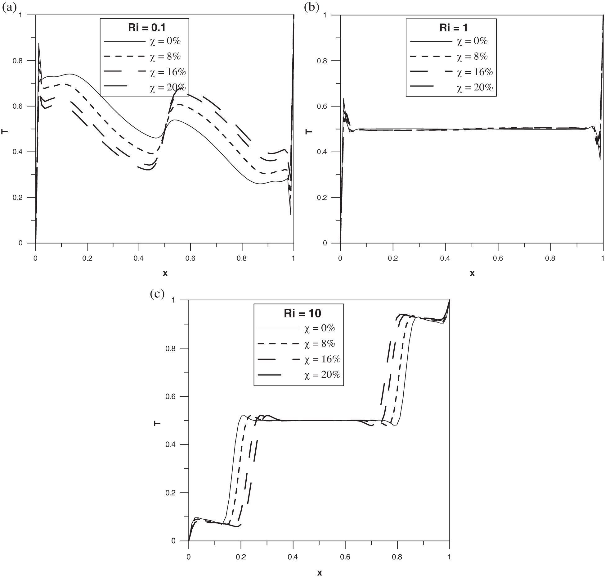
Figure 15: Horizontal mid-plane temperature profile: (a)
4.5 Effect of the Type of the Base Fluid
We shall now investigate the heat transfer inside the cavity under the conditions considered in this paper for different type of base fluids. For that, two additional base fluids are added to this study such as Methanol and Kerosene oil beside Water and Ethylene-glycol. Isotherms and streamline related to these fluids (Methanol and Kerosene) will not be presented since they are reminiscent to those obtained in the case of Water. However, drastic differences are obtained in terms of local and average Nusselt numbers. Figs. 16 and 17 show the evolution of the local Nusselt number on the left cold wall in the case of a pure fluid with no-nanoparticles and the case of a maximal nanoparticles volume fraction with
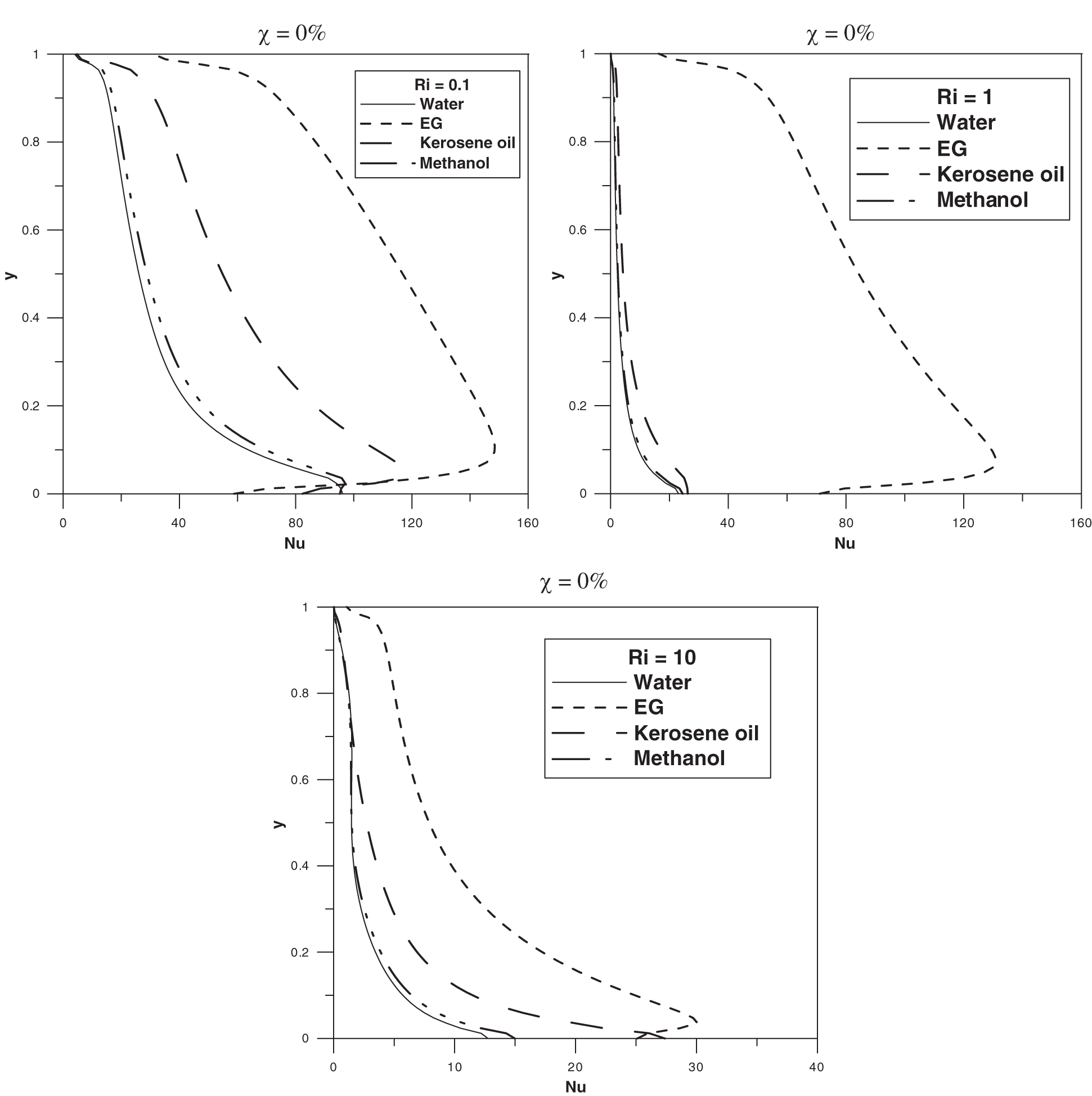
Figure 16: Local Nusselt number at the left wall for different values of Richardson number at
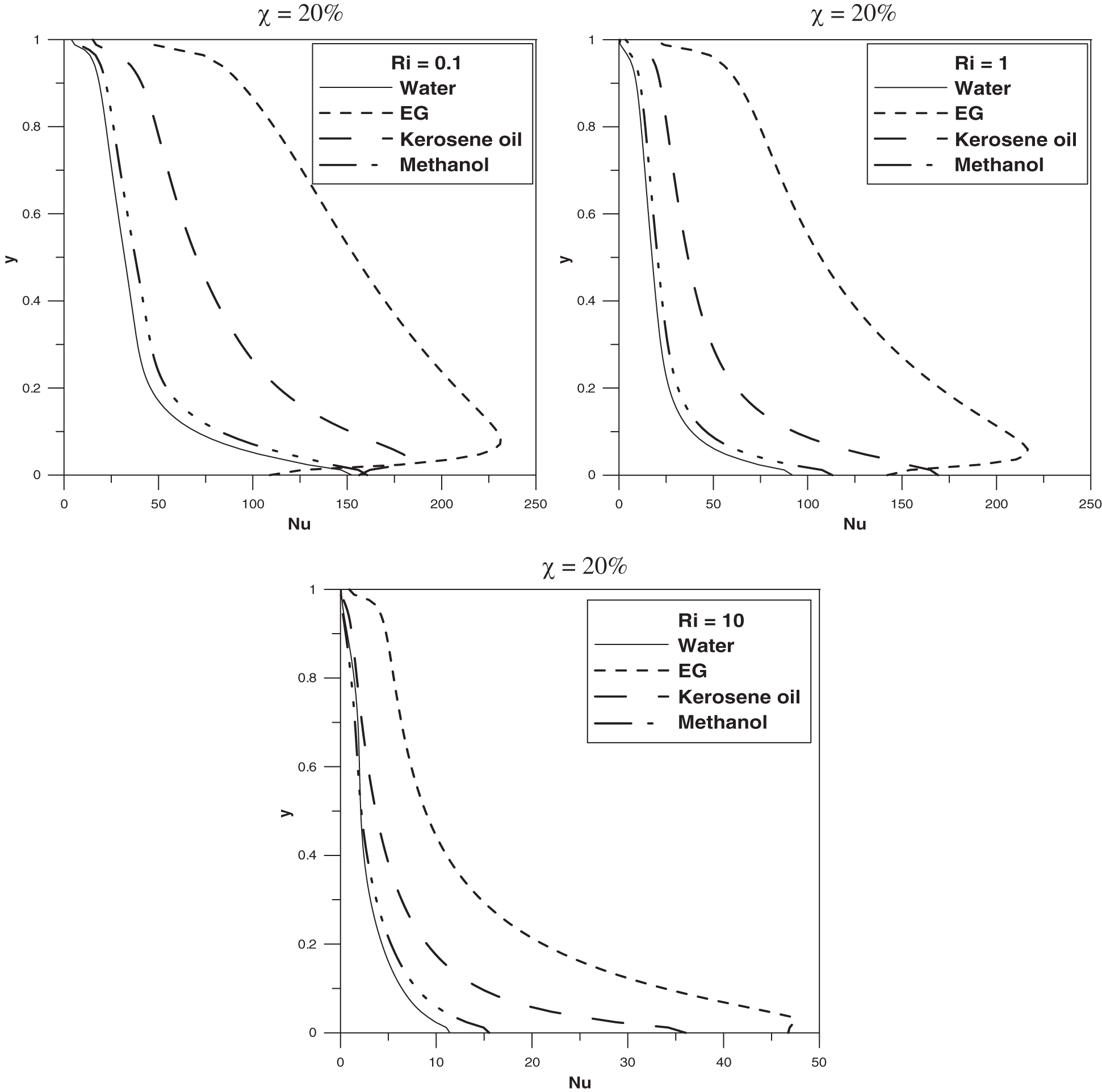
Figure 17: Local Nusselt number at the left wall for different values of Richardson number at
This maximum shifts gradually towards the top of the wall for the others fluids. In addition, it is apparent that the
In order to discern the effect of the Richardson number in the average Nusselt number,
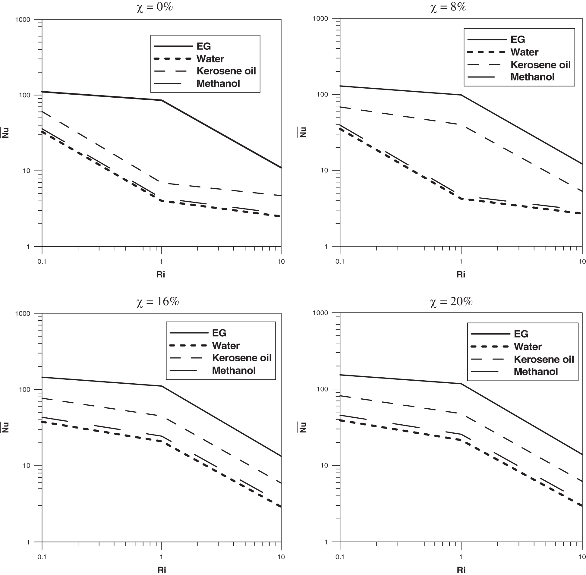
Figure 18: Average Nusselt number versus Richardson number for different volume fraction
Indeed, in the neighborhood of this value and in the case of Kerosene oil for example, an increase of the nanoparticles concentration to
4.6 Effect of the Nanoparticles Shape and Dynamic Viscosity Law
In this subsection, we attempt to shed light on the effect of the shape of the nanoparticles on the heat transfer using another thermal conductivity distribution involving cylindrical nanotubes particles given by the following expression:
In addition, a second dynamic viscosity model, that we term Model II, different to that described by Einstein expression (8) (Model I), is introduced. This model, stemmed from experimental characterizations and used by several authors in the literature [2], is given by
We consider the case of the Ag-water nanofluid with the volume fraction
In Fig. 19, we compare the average Nusselt number related to these shapes using these viscosity models. As one can notice, an enhancement of the heat transfer is observed using the spherical nanoparticles in comparison to the cylindrical ones. Also, a nearly constant decrease in the average Nusselt number vs. Ri is noticed using Model II. This is not the case when using Model I where this number,
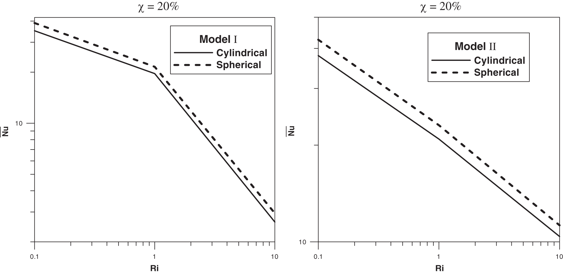
Figure 19: Average Nusselt number versus the Richardson number at
In this work, the mixed convection problem in a lid-driven square cavity filled with nanofluid is numerically investigated. The left and right vertical walls move up and down, respectively, and are held at two different temperatures while the horizontal walls are kept insulated. On the basis of the results presented in this paper, following findings may be summarized.
• The type of the nanoparticles does not affect the pattern formation in the system.
• Depending on the Richardson number range, the type of the nanoparticles has a significant role in the heat transfer in terms of both local and average Nusselt number.
• Different dynamics is observed when the Ethylene-glycol base fluid is used in comparison to water, methanol and kerosene oil.
• Ethylene glycol is the most convenient base fluid, ensuring maximum optimization of heat transfer in the cavity.
• The presence of nanoparticles always increases the heat transfer independently of neither the type of the nanoparticles nor the type of the base fluid.
• Increasing the Richardson number leads to a decrease in the heat transfer for the different mixtures.
• An improvement in heat transfer using spherical nanoparticles compared to cylindrical nanoparticles.
Funding Statement: The author received no specific funding for this study.
Conflicts of Interest: The authors declare that they have no conflicts of interest to report regarding the present study.
1. Tiwari, R. K., Das, M. K. (2007). Heat transfer augmentation in a two-sided lid-driven differentially heated square cavity utilizing nanofluids. International Journal of Heat and Mass Transfer, 50(9–10), 2002–2018. DOI 10.1016/j.ijheatmasstransfer.2006.09.034. [Google Scholar] [CrossRef]
2. Rana, P., Bhargava, R. (2011). Numerical study of heat transfer enhancement in mixed convection flow along a vertical plate with heat source/sink utilizing nanofluids. Communications in Nonlinear Science and Numerical Simulation, 16(11), 4318–4334. DOI 10.1016/j.cnsns.2011.03.014. [Google Scholar] [CrossRef]
3. Zeghbid, I., Bessaïh, R. (2017). Mixed convection in a lid-driven square cavity with heat sources using nanofluids. Fluid Dynamics & Materials Processing, 13(4), 251–273. [Google Scholar]
4. Bensouici, F., Boudebous, S. (2017). Mixed convection of nanofluids inside a lid-driven cavity heated by a central square heat source. Fluid Dynamics & Materials Processing, 13(3), 189–212. [Google Scholar]
5. Slama, S., Kahalerras, H., Fersadou, B. (2017). Mixed convection of a nanofluid in a vertical anisotropic porous channel with heated/cooled walls. Fluid Dynamics & Materials Processing, 13(3), 155–172. [Google Scholar]
6. Zaraki, A., Ghalambaz, M., Chamkha, A. J., Ghalambaz, M., de Rossi, D. (2015). Theoretical analysis of natural convection boundary layer heat and mass transfer of nanofluids: Effects of size, shape and type of nanoparticles, type of base fluid and working temperature. Advanced Powder Technology, 26(3), 935–946. DOI 10.1016/j.apt.2015.03.012. [Google Scholar] [CrossRef]
7. Raza, J., Farooq, M., Mebarek-Oudina, F., Mahanthesh, B. (2019). Multiple slip effects on MHD non-Newtonian nanofluid flow over a nonlinear permeable elongated sheet: Numerical and statistical analysis. Multidiscipline Modeling in Materials and Structures, 15(5), 913–931. DOI 10.1108/MMMS-11-2018-0190. [Google Scholar] [CrossRef]
8. Levin, M., Miller, M. (1981). Maxwell’s “treatise on electricity and magnetism.” Uspekhi Fizicheskikh Nauk, 135(11), 425–440. DOI 10.3367/UFNr.0135.198111d.0425. [Google Scholar] [CrossRef]
9. Peaceman, D. W., Rachford, J., Henry, H. (1955). The numerical solution of parabolic and elliptic differential equations. Journal of the Society for Industrial and Applied Mathematics, 3(1), 28–41. DOI 10.1137/0103003. [Google Scholar] [CrossRef]
10. Erturk, E., Gökçöl, C. (2006). Fourth-order compact formulation of Navier-Stokes equations and driven cavity flow at high Reynolds numbers. International Journal for Numerical Methods in Fluids, 50(4), 421–436. DOI 10.1002/fld.1061. [Google Scholar] [CrossRef]
11. Störtkuhl, T., Zenger, C., Zimmer, S. (1994). An asymptotic solution for the singularity at the angular point of the lid driven cavity. International Journal of Numerical Methods for Heat & Fluid Flow, 4(1), 47–59. DOI 10.1108/EUM0000000004030. [Google Scholar] [CrossRef]
12. de Vahl Davis, G. (1983). Natural convection of air in a square cavity: A bench mark numerical solution. International Journal for Numerical Methods In Fluids, 3(3), 249–264. DOI 10.1002/fld.1650030305. [Google Scholar] [CrossRef]
13. Markatos, N. C., Pericleous, K. (1984). Laminar and turbulent natural convection in an enclosed cavity. International Journal of Heat and Mass Transfer, 27(5), 755–772. DOI 10.1016/0017-9310(84)90145-5. [Google Scholar] [CrossRef]
14. Hadjisophocleous, G., Sousa, A., Venart, J. (1988). Prediction of transient natural convection in enclosures of arbitrary geometry using a nonorthogonal numerical model. Numerical Heat Transfer, Part A Applications, 13, 373–392. [Google Scholar]
15. El Bouihi, I., Sehaqui, R. (2012). Numerical study of natural convection in a two-dimensional enclosure with a sinusoidal boundary thermal condition utilizing nanofluid. Engineering, 4(08), 445–452. DOI 10.4236/eng.2012.48058. [Google Scholar] [CrossRef]
16. Khanafer, K., Vafai, K., Lightstone, M. (2003). Buoyancy-driven heat transfer enhancement in a two-dimensional enclosure utilizing nanofluids. International Journal of Heat and Mass Transfer, 46(19), 3639–3653. DOI 10.1016/S0017-9310(03)00156-X. [Google Scholar] [CrossRef]
17. Barakos, G., Mitsoulis, E., Assimacopoulos, D. (1994). Natural convection flow in a square cavity revisited: Laminar and turbulent models with wall functions. International Journal for Numerical Methods in Fluids, 18(7), 695–719. DOI 10.1002/fld.1650180705. [Google Scholar] [CrossRef]
18. Fusegi, T., Hyun, J., Kuwahara, K., Farouk, B. (1991). A numerical study of three-dimensional natural convection in a differentially heated cubical enclosure. International Journal of Heat and Mass Transfer, 34(6), 1543–1557. DOI 10.1016/0017-9310(91)90295-P. [Google Scholar] [CrossRef]
19. Goodarzi, M., Safaei, M., Karimipour, A., Hooman, K., Dahari, M. et al. (2014). Comparison of the finite volume and lattice Boltzmann methods for solving natural convection heat transfer problems inside cavities and enclosures. Abstract and Applied Analysis, 2014, 15. DOI 10.1155/2014/762184. [Google Scholar] [CrossRef]
20. Sharif, M. (2007). Laminar mixed convection in shallow inclined driven cavities with hot moving lid on top and cooled from bottom. Applied Thermal Engineering, 27(5–6), 1036–1042. DOI 10.1016/j.applthermaleng.2006.07.035. [Google Scholar] [CrossRef]
21. Waheed, M. (2009). Mixed convective heat transfer in rectangular enclosures driven by a continuously moving horizontal plate. International Journal of Heat and Mass Transfer, 52(21–22), 5055–5063. DOI 10.1016/j.ijheatmasstransfer.2009.05.011. [Google Scholar] [CrossRef]
22. Khanafer, K. M., Chamkha, A. J. (1999). Mixed convection flow in a lid-driven enclosure filled with a fluid-saturated porous medium. International Journal of Heat and Mass Transfer, 42(13), 2465–2481. DOI 10.1016/S0017-9310(98)00227-0. [Google Scholar] [CrossRef]
23. Iwatsu, R., Hyun, J. M., Kuwahara, K. (1993). Mixed convection in a driven cavity with a stable vertical temperature gradient. International Journal of Heat and Mass Transfer, 36(6), 1601–1608. DOI 10.1016/S0017-9310(05)80069-9. [Google Scholar] [CrossRef]
24. Cheng, T. (2011). Characteristics of mixed convection heat transfer in a lid-driven square cavity with various Richardson and Prandtl numbers. International Journal of Thermal Sciences, 50(2), 197–205. DOI 10.1016/j.ijthermalsci.2010.09.012. [Google Scholar] [CrossRef]
25. Riahi, M., Aniss, S., Ouazzani Touhami, M. (2019). Families of reversing and non-reversing Taylor vortex flows between two co-oscillating cylinders with different amplitudes. Physics of Fluids, 31(1), 014101. DOI 10.1063/1.5064656. [Google Scholar] [CrossRef]
26. Riahi, M., Aniss, S., Ouazzani Touhami, M., Skali Lami, S. (2016). Centrifugal instability of pulsed Taylor-Couette flow in a Maxwell fluid. European Physical Journal E, 39(8), 82. DOI 10.1140/epje/i2016-16082-9. [Google Scholar] [CrossRef]
27. Riahi, M., Aniss, S., Ouazzani Touhami, M., Skali Lami, S. (2015). Pulsed Taylor-Couette flow in a viscoelastic fluid under inner cylinder modulation. European Physical Journal Plus, 130(12), 253. DOI 10.1140/epjp/i2015-15253-7. [Google Scholar] [CrossRef]
28. Avila, M., Belisle, M. J., Lopez, J. M., Marques, F., Saric, W. S. (2008). Mode competition in modulated Taylor-Couette flow. Journal of Fluid Mechanics, 601, 381–406. DOI 10.1017/S0022112008000748. [Google Scholar] [CrossRef]
 | This work is licensed under a Creative Commons Attribution 4.0 International License, which permits unrestricted use, distribution, and reproduction in any medium, provided the original work is properly cited. |