| Fluid Dynamics & Materials Processing |
DOI: 10.32604/fdmp.2021.012108
ARTICLE
On Aircraft Lift and Drag Reduction Using V Shaped Riblets
1Aviation College of Northwestern Polytechnical University, Xi’an, 710072, China
2China Aerodynamic Research and Development Center, Mianyang, 621000
*Corresponding Author: Zihai Geng. Email: gzhlxqtt_11@163.com
Received: 15 June 2020; Accepted: 22 February 2021
Abstract: Reducing drag during take-off and nominal (cruise) conditions is a problem of fundamental importance in aeronautical engineering. Existing studies have demonstrated that v-shaped symmetrical riblets can effectively be used for turbulence control, with those with dimensionless depth h+ = 15 and dimensionless width s+ = 15 having the best drag reduction effect. In the present study, experimental tests have been conducted considering two models of the same size, one with smooth surface, the other with v-shaped riblets of the h+ = 15 and s+ = 15 type. The results show that for an angle of attack in the 8°~20° range (take-off stage), the maximum lift coefficient can be increased by 22%. For angle of attack between 8° and 14°, a drag reduction effect can be produced using riblets, which increases with the Reynolds number, leading to a decrease in the drag coefficient maximum of 36%. Flow visualization experiments have been carried out by means of Laser Induced fluorescence.
Keywords: Transport model; V-shaped riblet; lifting drag reduction; flow visualization
Since the 1970s, NASA Langely research centers discovered that tiny grooves in the flow direction of surfaces could effectively reduce wall friction, and researchers have carried out a lot of continuous research on drag reduction of riblets [1–3]. At present, according to the literature review, there is a conclusion: for the physical model of flat plate, the riblet of symmetrical V shape has the best drag reduction effect. When dimensionless sizes of the riblet are: the height h+ ≤ 25 and spacing s ≤ 30, drag reduction effect will occur. Moreover, when the range of the height of riblet, h+, is 8 to 15, the drag reduction effect was the best, which could reduce the turbulence frictional resistance by 3%~8% [4,5]. And there were many experiments that illustrated the phenomenon. For the Airbus plane with riblet surface, effect of 1%~2% fuel saving is achieved. Second, in the 1980s, German transport manufacturers applied an riblet surface to the plane which leading to 8% decrease in fuel cose [6–8]. Recently, Abdulbari et al. [9] studied the wall pressure fluctuations over the riblets using experiments. they found that spaced triangular riblets worked better than the triangular riblets.
Ho et al. investigated the stability of the laminar flow over streamwise riblets and oblique riblets experimentally [10]. Xie et al. [11] measured the drag acted on the van which was mounted with the riblet film, and drag-reducing effect can be observed.
In the actual flight of the transport, the take-off and climb stege focuses on lift augmentation, while the cruise phase concentrates on the drag-reducing effect. In recent years, the control of lift augmentation and drag reduction of riblet structure are also the research hotspots [12–14]. To quickly and effectively verify the lift augmentation and drag reduction effect of V-shaped flow riblet surface, the project team processed two 1:40 models in the systematic research on the aerodynamic characteristics of the conveyor model. In this work, the two models are tested. One is the transport with V-shaped symmetrical riblet on the surface including the body and wings. And the other is smooth surface. Under the same experimental conditions, the force measurement experiment was carried out to verify the lifting and drag reduction effect of the V-shaped symmetrical riblet surface, besides, the flow visualization experiment was carried out to demonstrated flow control effect of the riblets visually. And in the following parts, the force measurement experiments and the flow structure display experiments will be illustrated.
The experimental system consists of wind tunnel, water tunnel, transport model, force balance, data acquisition system, data analysis software, continuous laser and fluorescent agent, etc. The experimental test and data processing were carried out according to national industry standards. The force measurement experiments were carried out in the same wind tunnel whose size is 1.8 m (Width) × 1.4 m (Height). And the flow field visualization experiments were implemented in a 1 m × 1 m water tunnel. For a plane, the wing contributes to the lift mostly and the contribution of the part of body to the drag component is the most among all parts.
In this work, sizes and the configuration of the riblet are designed carefully, and under the experimental condition, the dimensionless height h+ is 15, besides which the dimensionless spacings of riblet is 15. In actual machining operation, there is a smooth transition between the riblet and the surface of the planes.
The current force measuring experiment was conducted in a 1.8 m × 1.4 m wind tunnel. The wind tunnel is a low-speed wind tunnel with open/close experimental section of backflow mode. The flow field indexes of the wind tunnel are shown in Tab. 1.
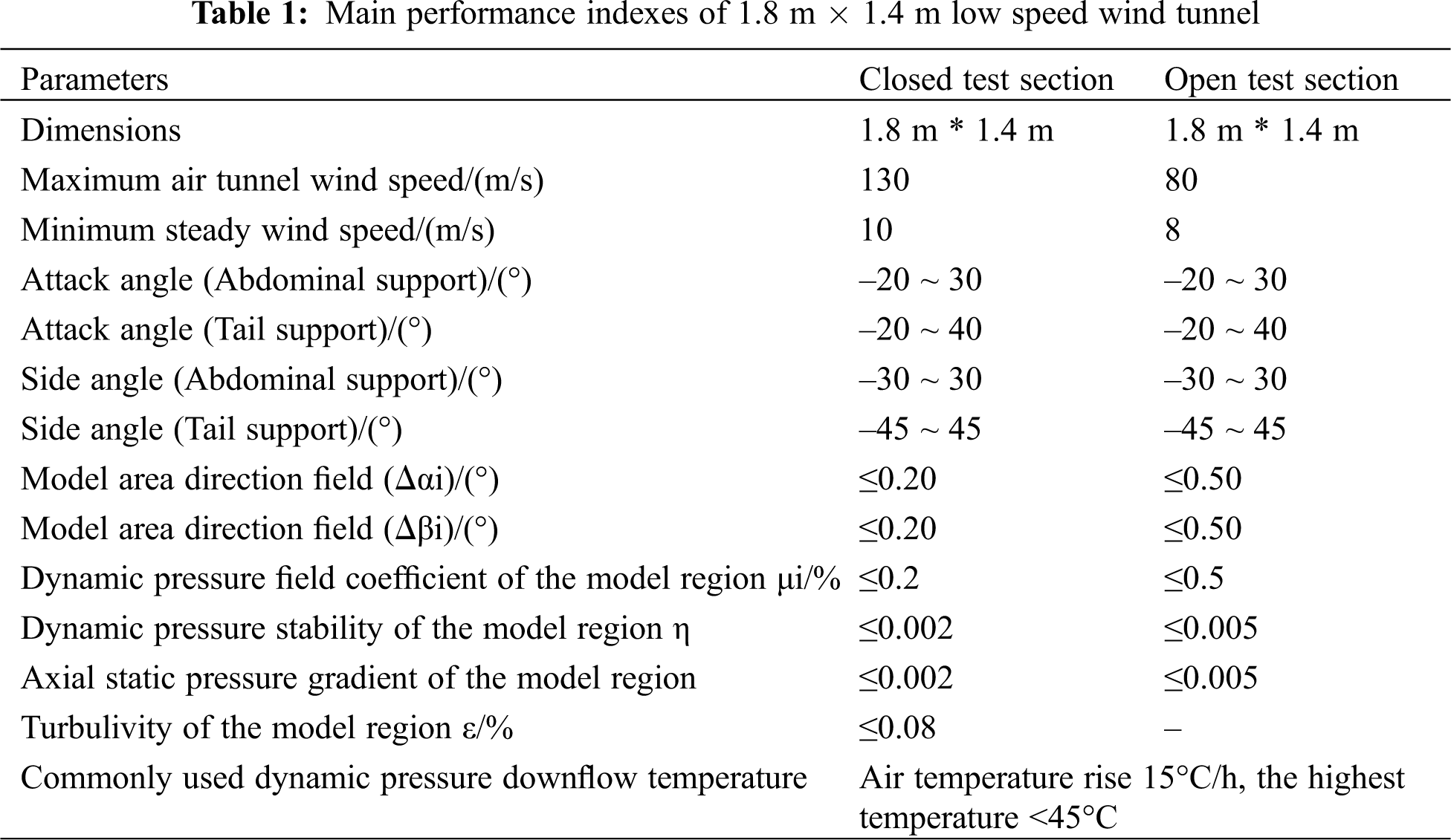
The model used in this experiment is the standard transport model with high-aspect ratio. The model was designed by the research team and processed by the First Transport Design and Research Institute of China Aviation Industry Corporation I. The scale of the model was 1:40 with whole metal structure. The profile drawing was shown in Fig. 1.
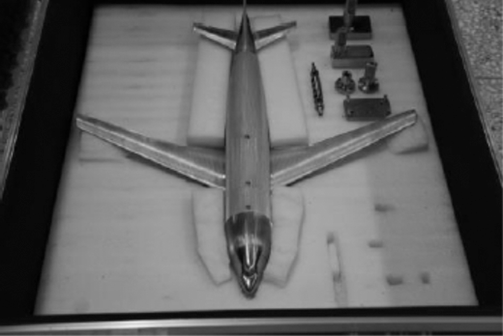
Figure 1: Full-transport mode
The model was supported by a belly strut in the 1.8 m × 1.4 m wind tunnel.
TG0201 bar structure force balance was used for force balance (as shown in Fig. 2), and the balance was installed in the model, as shown in Fig. 3.
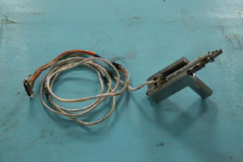
Figure 2: Bar structure force balance
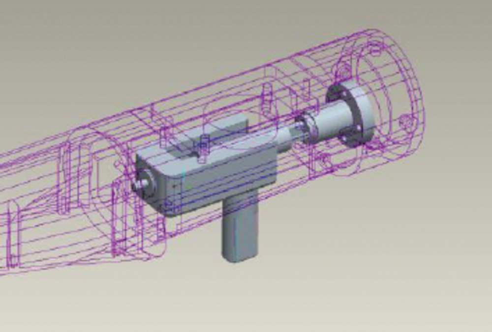
Figure 3: Balance installed in the model
2.4 Measurement and Control System
The 1.8 m × 1.4 m wind tunnel measurement and control system is based on computer network, mainly including data acquisition system, control system of angle of attack, velocity pressure control system, data processing system, experimental scheduling system and experimental analysis system. The data acquisition system was based on PXI data bus, which could be used for high-precision static data acquisition and high-precision and high-speed dynamic data acquisition. The wind tunnel had a velocity pressure control accuracy of less than 0.3% and an angle control accuracy of 0.05°.
The 1 m × 1 m low-speed water tunnel was a low-speed backflow water tunnel of which the test section has a completely open upper wall, as shown in Fig. 4. The water tunnel was horizontally arranged with the central axis of the loop of 18.71 m × 3.2 m and the contraction ratio is 9.3. The water tunnel consisted of an experimental section, an outlet sinking section, an axial flow pump power group, a reflux section (pipeline), a burst expansion energy dissipation section, a pre-contraction second-corner section, a steady flow and whole flow section, and a contraction section. A trailer with adjustable moving speed was arranged on the upper side of the experimental section. The whole loop of the tunnel is made of 3.4# stainless steel. And the lower wall and side wall of the experiment section were tempered glass of which the light transmittance is better than 0.9.
The range of the flow speed of water tunnel in the experiment section is 0.1 to 1 m/s. And the common flow velocity is 0.1 to 0.5 m /s, besides, the turbulivity in the model area was ε ≤ 0.1% (0.1~0.3 m/s), ε ≤ 0.2% (0.3~0.5 m/s) and ε < 0.5% (0.5~1 m/s).

Figure 4: Hydrodynamic outline of 1 m × 1 m water tunnel
3 Experiment Details and Methods
Two full transport models were used, including one smooth surface and one flow riblet surface, as shown in Fig. 5. The experiment was carried out with steady velocity pressure, and the calculation formula of dynamic pressure was q = 1/2ρv2. The Reynolds number was changed under the experimental state of wind speed of 20 m/s, 30 m/s, 40 m/s, 50 m/s, 60 m/s and 70 m/s. The corresponding dynamic pressures were 234 Pa, 527 Pa, 936 Pa, 1462.5 Pa, 2106 Pa and 2866.5 Pa, with an attack angle of 0°~20° with the interval of 2°.
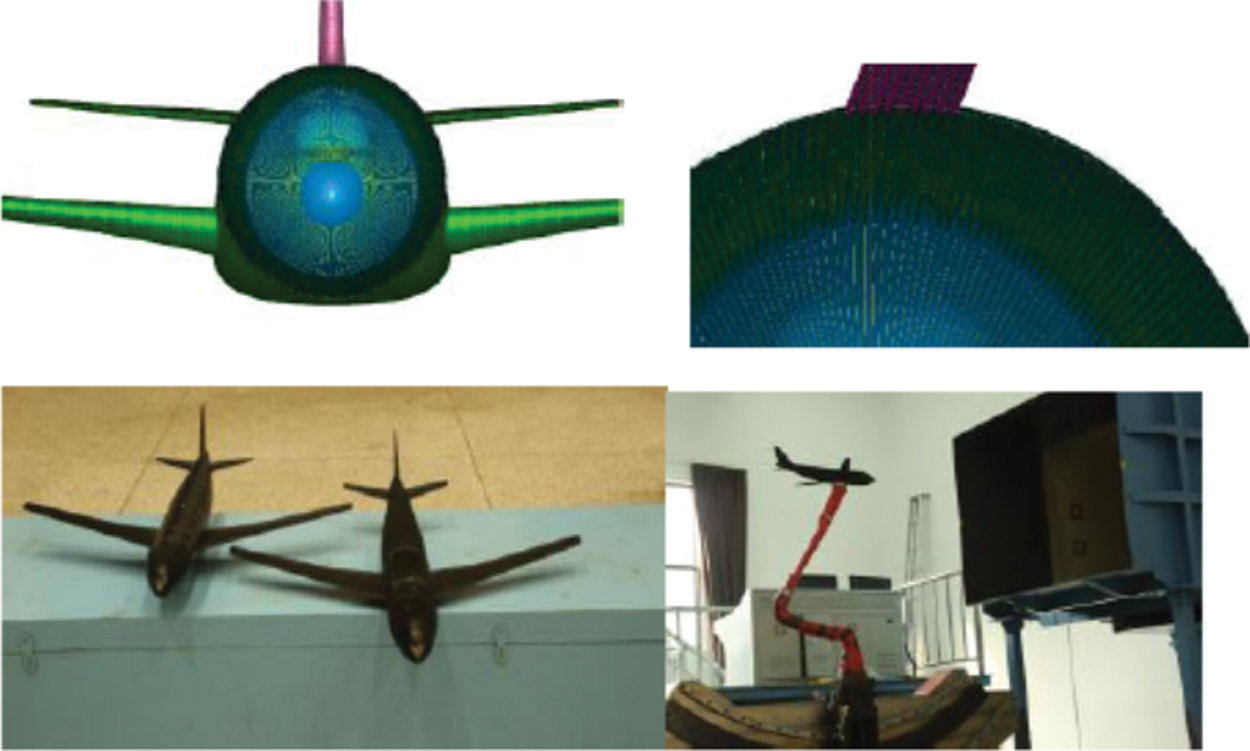
Figure 5: Whole transport models with smooth surface and riblet surface
3.2.1 Model Inspection and Installation
During the preparation of the experiment, the model should be assembled and tested on the platform, including the measurement of the installation position of each component of the model and the measurement of the installation position of the balance, etc. The measurement results will be recorded for subsequent verification.
Before experiment, the balance and the relative instruments need to be calibrated. If conditions permit, the balance should be installed on the ground for adaptability test. After the balance/model system is installed into the test section, necessary adaptability tests should also be conducted to ensure the system is installed in the proper position and correct the installation error.
The model is installed in the center of the 1.8 m × 1.4 m wind tunnel section with a belly strut system.
And the initial attitude angle error should be less than 3’. After the model is fixed and connected with the strut, the initial roll angle may be generated. If the roll angle was large, the test results should be corrected accordingly. The initial elastic angle of the support system in the direction of attack and roll should also be measured after the model is installed.
The experimental data were collected by PXI system. The test was completed by step method. The sampling method was tentatively set as: sampling delay of 5 s, sampling time of 8 s, sampling frequency of 500 Hz in each channel. The noise reduction method based on the wavelet analysis theory was used to process the original signal.
Experimental results shafting was defined as follows:
Model body shafting: the origin was at the model moment reference center, the X axis was parallel to the model axis, pointing in front direction. And the Z axis was inside the model symmetry plane, perpendicular to the X axis, pointing down, besides, the Y axis was perpendicular to the ZOX plane, pointing to the right.
Model wind shafting: the origin was the same as the model body shafting, the X-axis was opposite to the incoming flow direction, the Z-axis was in the symmetry plane of the model, perpendicular to the X-axis and pointing down, and the Y-axis was perpendicular to the ZOX plane and pointing to the right.
Balance coordinate system: the origin was in the center of the balance, the X-axis was parallel to the model axis, pointing in front direction, the Y-axis was inside the model symmetry plane, perpendicular to the X-axis, pointing up, and the Z-axis was perpendicular to the XOY plane, pointing to the right.
Three sets of experimental results were given as the form of the six-component data, one set in the form of model body shafting, one set in the form of model wind shafting, one set in mixed shafting, lift coefficient and drag coefficient in model wind shafting, and the other four quantities in model body shafting. The data storage format was stored in 8 columns according to the conventional data format of force measurement experiment:
The model body axis coefficients were arranged in the following order: CN, CA, Cm, CY, Cn, Cl, α and β where CN denotes the normal force coefficient, CA denotes the axial force coefficient, Cm denotes the pitching moment coefficient, CY denotes the transverse force coefficient, Cn denotes the yawing moment coefficient, Cr denotes the rolling moment coefficient, α denotes the angle of attack, and β denotes the sideslip angle.
The wind axis coefficients of the model were arranged in the following order: CL, CD, Cma, Cc, Cna, Cla, α and β. Where CL denotes the lift coefficient, CD denotes the resistance coefficient, Cma denotes the pitching moment coefficient, Cc denotes the lateral force coefficient, Cna denotes the yawing moment coefficient, Cla denotes the rolling moment coefficient, α denotes the angle of attack, and β denotes the sideslip angle.
The mixed axis coefficients were arranged in the following order: CL, CD, Cm, CY, Cn, Cl, α and β. Where CL denotes the lift coefficient, CD denotes the drag coefficient, Cm denotes the pitching moment coefficient, CY denotes the transverse force coefficient, Cn denotes the yawing moment coefficient, Cl denotes the rolling moment coefficient, α denotes the angle of attack, and β denotes the sideslip angle.
As for the final test data, the processing data should also be provided to correct the errors cause by the bracket and the hole in wall. Hence, the following data is needed, they are the results of unfastened bracket and the wall hole interference correction, the correction of the existence of fastened bracket, the results of only hole wall interference correction, and the data of hole wall interference correction and fastened bracket.
The experimental data processing was carried out according to the conventional method, including deducting the initial reading, balance load calculation and angle correction, balance shaft rotation axis, conversion coefficient, fastened bracket interference, body shaft rotation axis, hole wall interference correction and data shafting conversion. There were some differences between the two steps of deducting the initial reading as well as the shaft of the balance shafting turning model, and the standard procedures.
4.3.1 Number of Blows-Initial Reading
The blow number minus initial reading was substituted into the balance formula, and the measured load of the balance was calculated by iteration (generally seven times) according to the requirements, with the unit of N.
It should be noted that, since the model attack angle changed when the wind tunnel worked, the data needed to be compared with that when the wind tunnel stopped. And the difference could be found after interpolation of the data from the balance system and data analysis system. The outputs of the balance included NT (normal force), AT (axial force), mT (pitching moment), YT (transverse force), nT (yaw moment) and lT (roll moment).
The angle correction formula is:
α denotes the measured real-time angle of inclination sensor A1, β denotes the nominal side slipping angle of the model, Δαe and Δβe are the balance elastic angles determined by the balance load calculated from the blow number minus the initial reading, respectively. Δαp and Δβp represents the average flow deflection angles of the wind tunnel.
4.3.3 Rotary Axis of Balance Axis
Step 1: Coordinate translation. The origin of the balance shafting needs to be transformed to the origin of the model:
where FT = [AT NT YT]T, and it denotes the force measured by the balance; MT = [lT nT mT]T, the moment measured by the balance. F’T = [−AT NT YT]T, PT = [x0 y0 z0]T, where x0, y0 and z0 referred to the coordinates of the model moment reference point in the balance coordinate system By expanding the equation,
Step 2: Coordinate frame rotation. eliminated the influence of installation error and elastic deformation angle. It should be clear that the model body shafting did not coincide with the balance coordinate system after coordinate rotation. The order was converted to βR, αR and γR, i.e.,
where, Ft = [−At Nt Yt]T is the the force measured by the balance after deducting installation error and elastic deformation angle; FTm = [−Atm Ntm Ytm]T, mmT rep the coordinate rotation transformation matrix, which could be expressed as,
with
And this term is the representation of the moment measured by the balance after deducting the installation error and elastic deformation. By expanding the equation,
where, the subscript “t” represented the expression form of the load measured by the balance in the model coordinate system. αtotation, βtotation and γtotation referred to the included angle between the model coordinate axis and the calibration axis of the balance (the fixed end of the balance), which could be decomposed into three parts, namely,
Under the condition of no load, for αA, βA and γA, the three initial installation angles of the model is measured [4]. And Δα0, Δβ0, and Δγ0 denotethe elastic deformation angle caused by gravity of the model, which was calculated according to the initial condition and the state with model. The initial condition is representing that the model is installed in the wind tunnel at zero αA. And the zero reading is that the model is at an attack angle of 0° on the platform.
Δαelasticity, Δβelasticity and Δγelasticity denotes the extra angle of attack caused by deformation. When the data of attitude angle of the model and the change of the aerodynamic load of the model is obtained, the elastic deformation angle can be generated, which is as the following:
When the ground test is finished, the zero position of the balance should be recorded. Before the measurement, the model should be installed on the platform.
4.3.5 Model Wind Shafting to Model Body Shafting Conversion
The calculation formula of the coefficient was as follows:
Figs. 6 and 7 show that the lift and drag of different scaled models in different wind tunnels. The results suggest that the experimental results of different scaled standard models in different wind tunnels are in accordance with the theory. CLmax and αcr increase with the experimental Re number, and CDmin shows a decreasing trend, because the maximum lift coefficient and the minimum drag coefficient were closely related to Reynolds number.
Figs. 8 to 15 showed the lift and drag characteristics of smooth and riblet-surface model under different experimental wind speed conditions. It could be observed from Fig. 8 that under the incoming flow wind speed of 30 m/s, the smooth surface and the riblet surface had the same trend in lift coefficient. Under a small attack angle, the riblet surface had lift-augmentation effect, with a 6% increase in maximum lift coefficient. It could be identified from Fig. 8 that under the condition where the wind speed was 30 m/s, the flow channel had no obvious drag reduction effect.
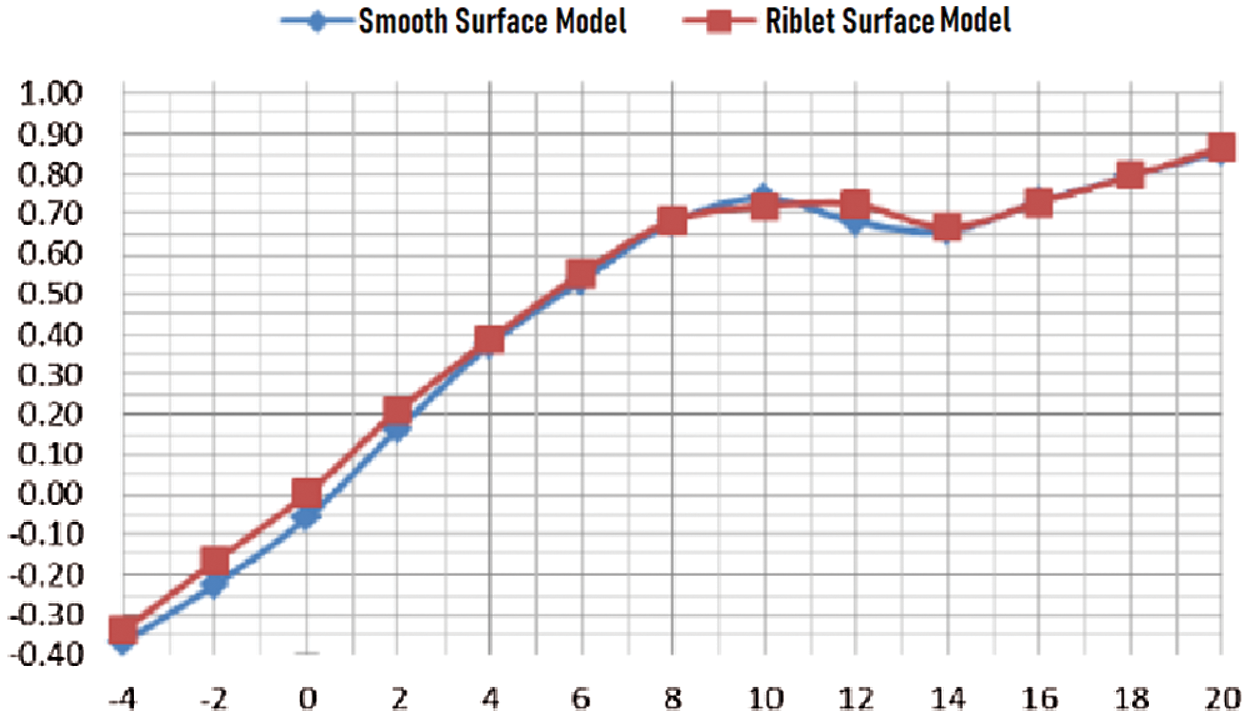
Figure 6: Lift coefficient curve under wind speed of 30 m/s
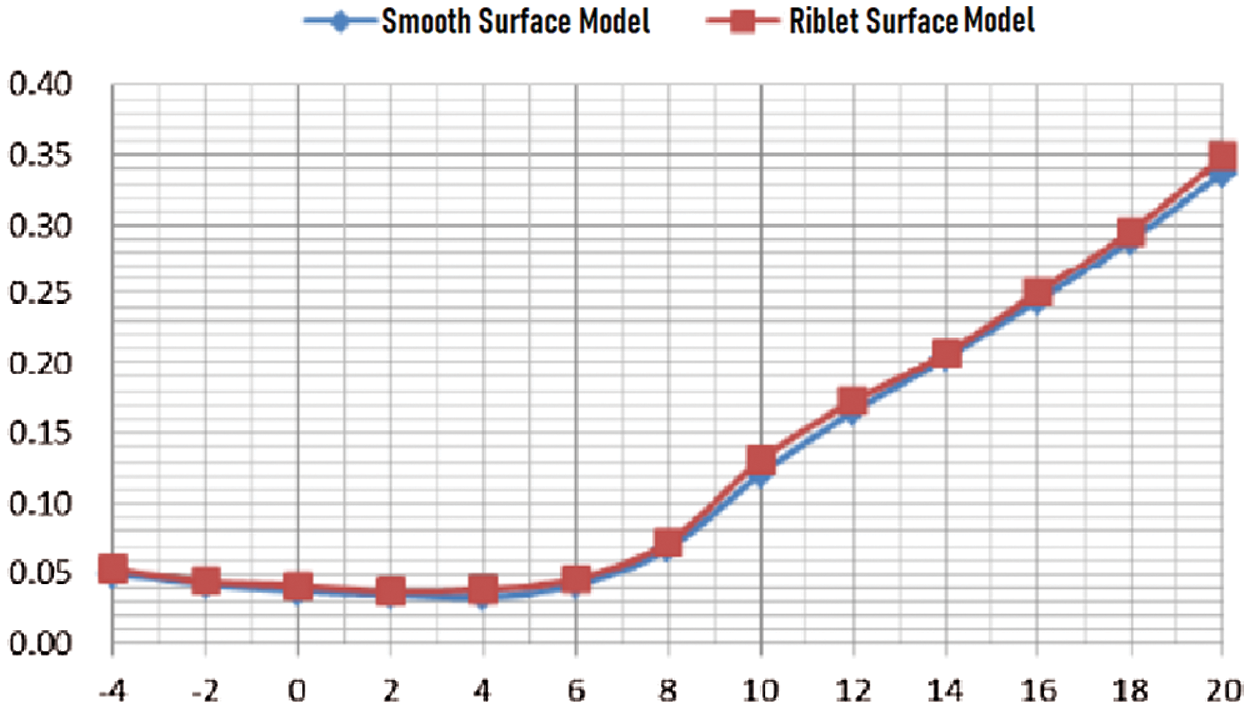
Figure 7: Drag coefficient curve under wind speed of 30 m/s
It could be identified from Fig. 8 that under the flow speed of 40 m/s, the smooth surface and the riblet surface had the same trend in lift coefficient. Under the attack angle of 6°~16°, the riblet surface had obvious lift-augmentation effect, with a 6% increase in maximum lift coefficient. It can be seen from Fig. 9 that at an attack angle of 8°~10°, the flow riblet had a drag reduction effect, with a 7% decrease in drag.
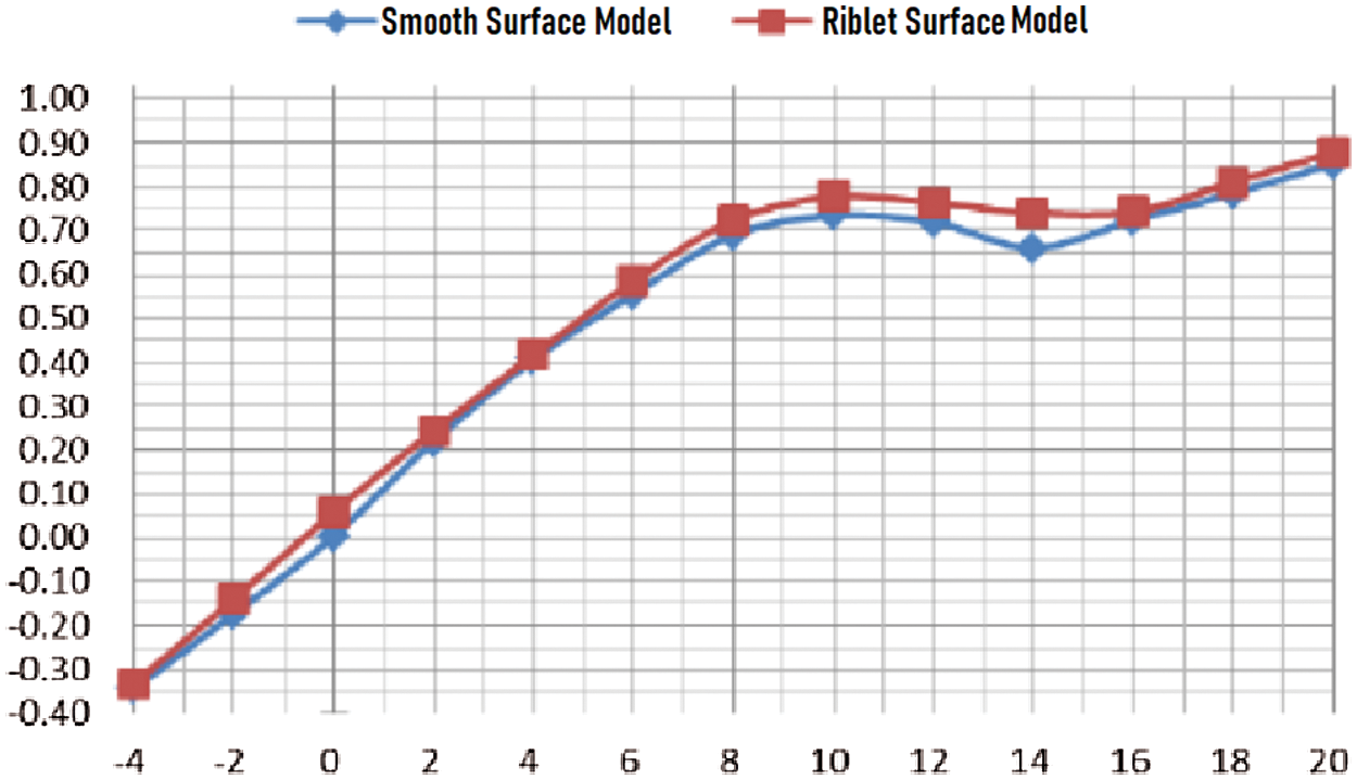
Figure 8: Lift coefficient curve under wind speed of 40 m/s
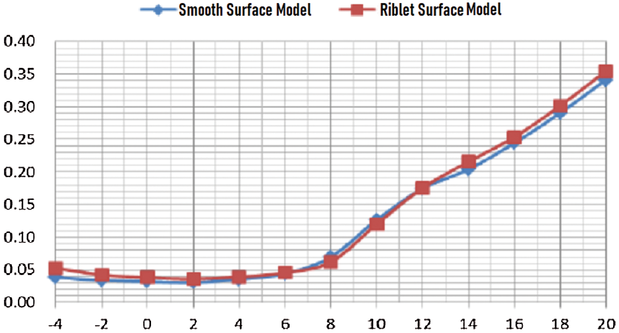
Figure 9: Drag coefficient curve under wind speed of 40 m/s
It could be identified from Fig. 10 that under the incoming flow wind speed of 50 m/s, the smooth surface and the riblet surface had the same law of lift coefficient curve. Under the attack angle of 6°~18°, the riblet surface had obvious lift-augmentation effect, with a 9% increase in maximum lift coefficient. It can be seen from Fig. 11 that at an attack angle of 8°~12°, the flow riblet had a significant drag-reduction effect, with a 7% decrease in drag.
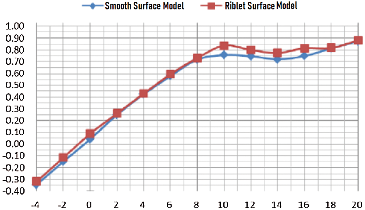
Figure 10: Lift coefficient curve under wind speed of 50 m/s
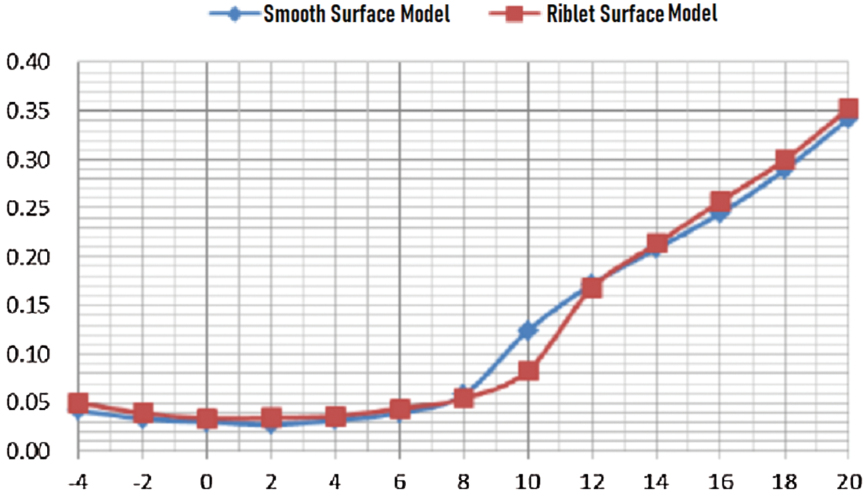
Figure 11: Drag coefficient curve under wind speed of 50 m/s
It could be identified from Fig. 12 that under the incoming flow wind speed of 60 m/s and the attack angle of 6°~18°, the riblet surface had obvious lift-augmentation effect, with a 12% increase in maximum lift coefficient. It can be seen from Fig. 13 that at an attack angle of 8°~12°, the flow riblet had a significant drag-reduction effect, with a 33% decrease in drag.
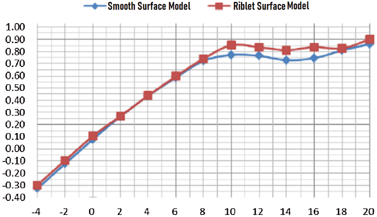
Figure 12: Lift coefficient curve under wind speed of 60 m/s
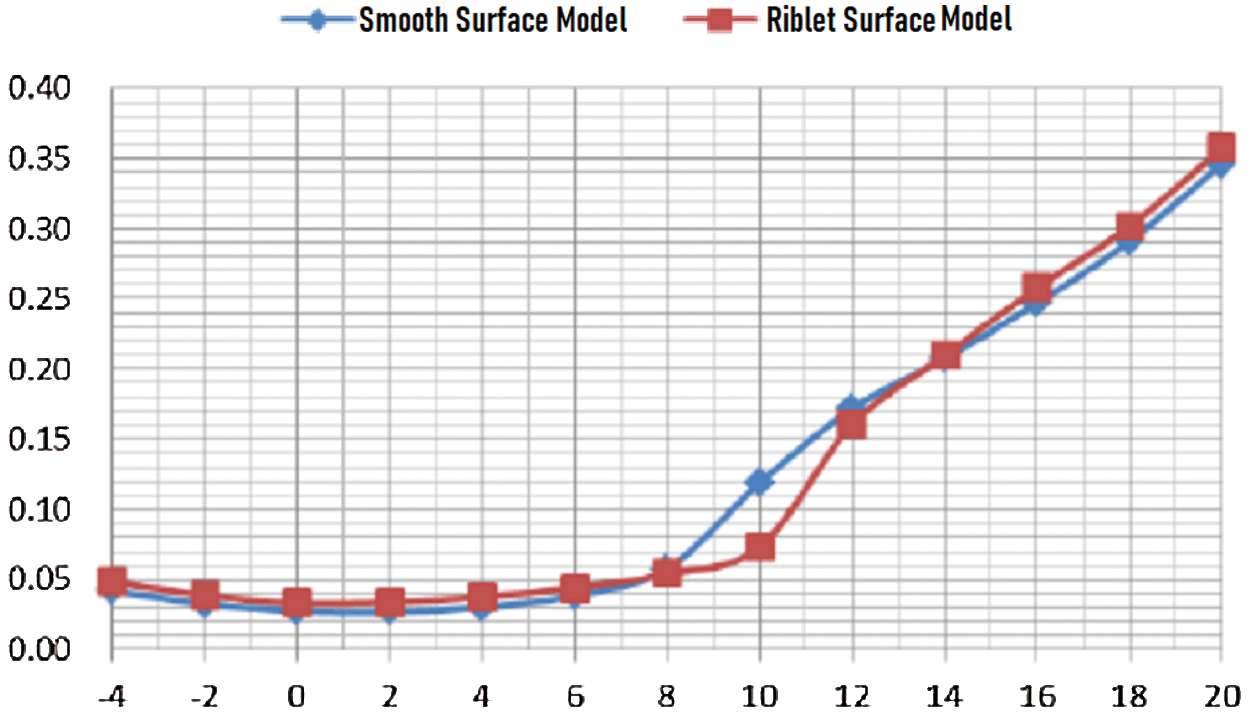
Figure 13: Drag coefficient curve under wind speed of 60 m/s
It could be observed from Fig. 14 that under the condition of flow speed of 70 m/s and the attack angle of 8°~20°, the riblet surface had obvious lift-augmentation effect with a 22% increase in maximum lift coefficient. It can be seen from Fig. 15 that at an attack angle of 8°~14°, the flow riblet had a significant drag reduction effect, with a maximum drag coefficient reduction of 36%.
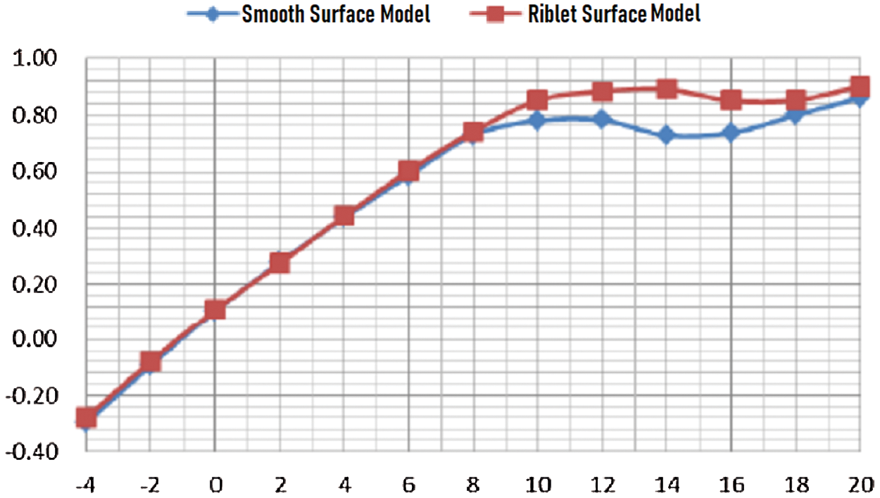
Figure 14: Lift coefficient curve under wind speed of 70 m/s
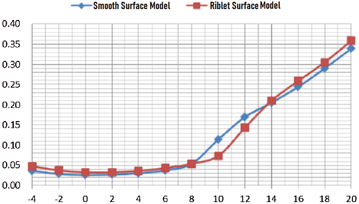
Figure 15: Drag coefficient curve under wind speed of 70 m/s
According to the analysis of lift coefficient curve, at the attack angle of 8°~20°, the V-shaped riblet wing surface has the lift-augmentation effect under the experimental condition that the flow speed are 30 m/s, 40 m/s, 50 m/s, 60 m/s and 70 m/s. The lift-augmentation effect increases with the increase of Reynolds number. Under the condition of flow speed of 70 m/s and the attack angle of 14°, the lift coefficient increases by 22%, making a large contribution to take-off and climb.
According to the analysis of the drag coefficient curve, under the condition offlow speed of 30 m/s, the V-shaped riblet wing surface had little drag reduction effect. When theflow speed are 40 m/s, 50 m/s, 60 m/s and 70 m/s, the model’s attack angle ranges from 8° to 14°, and the drag reduction effect of riblets appears, which increased with the Reynolds number. Under the incoming flow wind speed of 70 m/s and the attack angle of 10°, the drag coefficient is reduced by 36%, making a large contribution to take-off and climb.
Figs. 16 to 20 showed the experimental results of flow structure around smooth wing surface and riblet wing surface at the same experimental velocity and different attack angles. It could be observed from Fig. 18 that there was a classical flow instability structure in the wake field of smooth wing surface at the attack angle of 0°. In the same experimental condition, the flow instability was inhibited on the riblet wing surface and in the wake field structure.
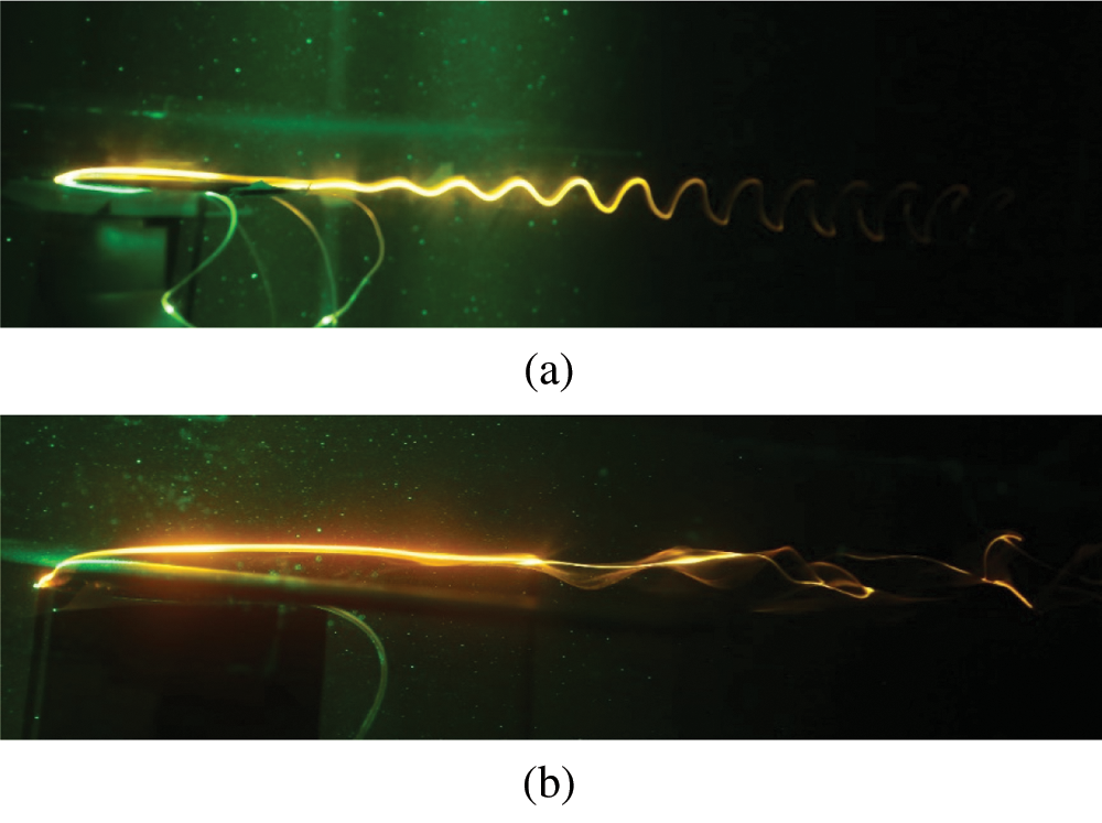
Figure 16: Wing surface and wake structure under α = 0° (a) Smooth surface (b) Riblet surface
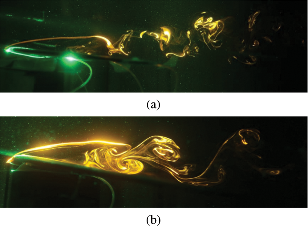
Figure 17: Wing surface and wake structure under α = 8° (a) Smooth surface (b) Riblet surface
By comparing the different flow structures on the smooth wing surface and the riblet wing surface, it was clear that the riblet wing surface had an obvious inhibitory effect on the flow separation under the model’s attack angle of 8°.
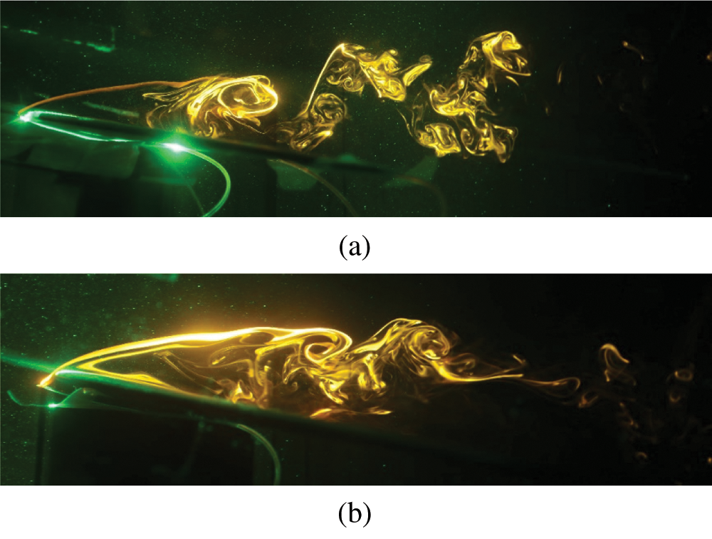
Figure 18: Wing surface and wake structure under α = 10° (a) Smooth surface (b) Riblet surface
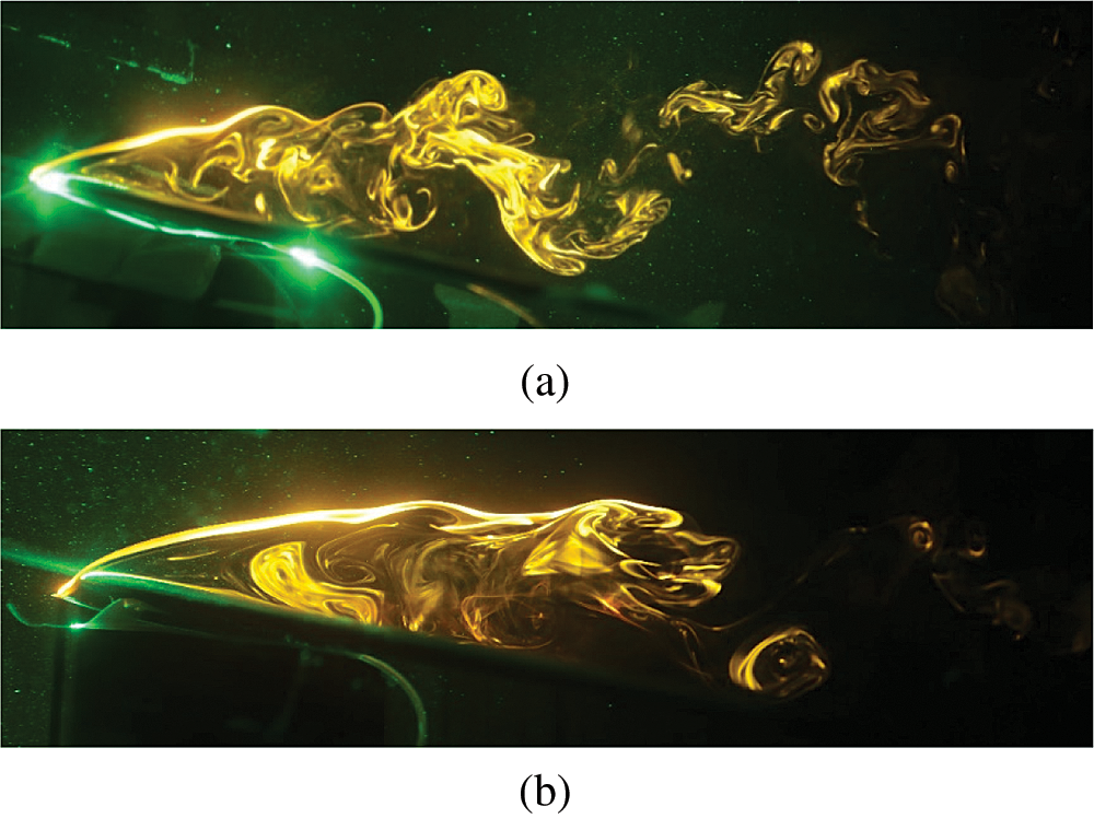
Figure 19: Wing surface and wake structure under α = 12° (a) Smooth surface (b) Riblet surface
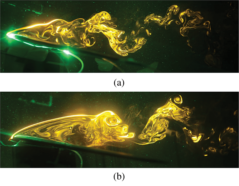
Figure 20: Wing surface and wake structure under α = 14° (a) Smooth surface (b) Riblet surface
It could be observed from Fig. 17 that under the attack angle of 8°, the flow structure around the smooth wing surface was clear, the flow was separated from the leading edge of the wing, and the vortex structure in the wake field was clear. In the same experimental condition, the reattachment structure appeared in the leading edge separation line of the riblet wing surface, and the vortex structure in the wake field was stable.
Fig. 18 shows the comparison results of flow around structures of the two wing surfaces at the attack angle of 10°. It could be observed that the leading edge separation line on the smooth wing surface continued to develop in the direction away from the wing surface. The vortex shedding structure in the wake field caused vortex rupture area to expand in the far field and approach to the trailing edge of the wing. The attached flow area on the flow channel surface of the wing decreased, and the multi-scale vortex structure was stable.
Fig. 19 indicated that under the model’s attack angle of 12°, the vortex rupture position in the wake field of the smooth wing reached the trailing edge of the wing. The vortex breakdown position in the wake field of the flow riblet wing was far from the trailing edge.
Fig. 20 indicates that under the model’s attack angle of 14°, in the wake field of a smooth wing, the vortex rupture was advanced from the trailing edge to the leading edge of the wing. The vortex breakdown position in the wake field of the flow channel wing approach to the trailing edge of the wing.
1) The force measurement experimental results illustrate that the lift-drag characteristics of different models and different wind tunnel transport models were consistent, and the experimental results were reliable.
2) Under the condition of flow speed of 30 m/s, 40 m/s, 50 m/s, 60 m/s and 70 m/s and within the attack angle of 8°~20°, the V-shaped flow riblet wing had an obvious lift-augmentation effect, which increased with Reynolds number. When the flow speed is 70 m/s, the increase of lift coefficient was largest with a 22% increase in maximum lift coefficient, and the angle of attack was in the phase of take-off climb.
3) Under the condition of flow speed of 40 m/s, 50 m/s, 60 m/s and 70 m/s, the model’s attack angle ranged from 8° to 14°, and the drag reduction effect existed for the riblet model. Under the incoming flow wind speed of 70 m/s and the attack angle of 10°, the drag coefficient is reduced by 36%, making a large contribution to take-off and climb.
4) In the range of attack angle during take-off climb, the V-shaped symmetrical flow riblet surface had obvious inhibitory effect on the wing surface separation and the vortex breakage in the wake field.
Funding Statement: The authors received no specific funding for this study.
Conflicts of Interest: The authors declare that they have no conflicts of interest to report regarding the present study.
1. Wang, J. J., Chen, G. (2001). Experimental studies on the near wall turbulent coherent structures over riblets surfaces. Journal of Aviation, 5(22), 400–405. [Google Scholar]
2. Wang, J. (1998). A review of studies on turbulent drag reduction of riblet surface. Journal of Beijing University of Aeronautics and Astronautics, 24(1), 31–34. [Google Scholar]
3. Li, Y., Qiao, Z., Wang, Z. (1995). An experimental research of drag reduction using riblets for the y-7 airplane. Journal of Experiments in Fluid Mechanics, 9(3), 21–26. [Google Scholar]
4. Sasamori, M., Mamori, H., Iwamoto, K., Murata, A. (2014). Experimental study on drag-reduction effect due to sinusoidal riblets in turbulent channel flow. Experiments in Fluids, 55, 1828. [Google Scholar]
5. Sundaram, S., Viswanath, P. R., Rudrakumar, S. (1996). Viscous drag reduction using riblets on a NACA0012 airfoil to moderate incidence. AIAA Journal, 34(4), 676–682. [Google Scholar]
6. Viswanath, P. R. (2002). Aircraft viscous drag reduction using riblets. Progress in Aerospace Sciences, 38(6–7), 571–600. [Google Scholar]
7. Wang, X. (2002). Experiment of low speed wind tunnel. Beijing: National Defense Industry Press. [Google Scholar]
8. Khar, M. I., Ahasan, K., Ali, M. (2018). Numerical investigation of drag reduction using moving surface boundary layer control (MSBC) on NACA, 0012 airfoil. AIP Conference Proceedings, 1980(1), 040011. [Google Scholar]
9. Abdulbari, H. A., Mahammed, H. D., Hassan, Z. (2016). Wall-pressure fluctuations of modified turbulent boundary layer with riblets. Fluid Dynamics & Materials Processing, 12(2), 86–101. [Google Scholar]
10. Ho, H. Q., Asai, M. (2018). Experimental study on the stability of laminar flow in a channel with streamwise and oblique riblets. Physics of Fluids, 30, 024106. [Google Scholar]
11. Xie, X., Cao, L., Huang, H. (2018). Thickened boundary layer theory for air film drag reduction on a van body surface. AIP Advances, 8, 055129. [Google Scholar]
12. Bilinsky, H. C., Wilson, R. N. (2018). Maturation of direct contactless microfabrication for application of drag reducing riblets. 2018 AIAA Aerospace Sciences Meeting. [Google Scholar]
13. Takahashi, H., Iijima, H., Kurita, M., Koga, S. (2018). Evaluation of skin friction drag reduction in turbulent boundary layer using riblets. Applied Sciences, 9(23), 5119. [Google Scholar]
14. Catalano, P., Donato, D. D., Mele, B., Tognaccini, R., Moens, F. (2018). Effects of riblets on the performances of a regional aircraft configuration in NLF conditions. AIAA Aerospace Sciences Meeting, pp. 1–16. Kissimmee, USA. [Google Scholar]
 | This work is licensed under a Creative Commons Attribution 4.0 International License, which permits unrestricted use, distribution, and reproduction in any medium, provided the original work is properly cited. |