Fluid Dynamics & Materials Processing

DOI: 10.32604/fdmp.2021.016081

ARTICLE

An Experimental Study on the Void Fraction for Gas-Liquid Two-Phase Flows in a Horizontal Pipe

Li Lei1, Jun An1, Fushun Liang1, Cheng Cheng1, Naixiang Zhou2, Yanhong Ning3 and Jingzhi Zhang1,4,*

1School of Energy and Power Engineering, Shandong University, Jinan, 250061, China
2Shandong Urban and Rural Planning and Design Institute, Jinan, China
3China National Petroleum Corporation Jichai Power Co., Ltd., Jinan, China
4Shenzhen Research Institute of Shandong University, Shenzhen, China
*Corresponding Author: Jingzhi Zhang. Email: zhangjz@sdu.edu.cn
Received: 04 February 2021; Accepted: 26 May 2021

1  Introduction

With the development of science and technology, industrial equipment has gradually shown a trend of miniaturization. Micro-chemical technology [1,2] has become an emerging interdisciplinary, and the corresponding gas-liquid two-phase flow in small channels has also attracted more and more attention.

The flow pattern is the basis of studying two-phase flow. In the past few decades, many scholars [3–5] have conducted a lot of experimental research and observed some flow patterns, such as bubbly flow, dispersed bubbly flow, slug flow, stratified flow, annular flow and mist flow. Some researchers have proposed flow regime maps based on experimental data. Compared with conventional channels, the area/volume ratio of small channels is greatly increased, and the influence of surface tension and viscous force is significantly enhanced, which means that some flow characteristics and parameter change laws shown in small channels are different from those of conventional channels. The flow pattern transition boundary of the small channel has also changed. Barnea et al. [3] used a horizontal tube with a diameter of 4–12.3 mm to observe seven flow patterns: smooth stratified flow, wave stratified flow, elongated bubbly flow, slug flow, annular flow, wave annular flow, and dispersed bubbly flow. Ong et al. [6] measured the two-phase flow pattern in a horizontal circular tube with an inner diameter of 1–3 mm, and classified it into isolated bubbles, coalesced bubbles, wave annular flow and smooth annular flow. Sudarja et al. [7] found five flow patterns in a circular tube with an inner diameter of 1.6 mm, namely slug flow, plug flow, slug-annular flow, annular flow and agitated flow. Compared with conventional tubes, the proportion of annular flow on the flow pattern map is higher for small channels. On the contrary, the proportion of stratified flow decreases with decreasing channel sizes because of the low gravity effect.

As one of the important parameters of two-phase flow, the void fraction directly affects the pressure drop, heat transfer coefficient and the flow pattern of gas-liquid two-phase flow. Accurate calculation and prediction of the void fraction of gas-liquid two-phase flow are of great significance to the design of engineering systems. Compared with the traditional quick closing valves method [8], the acoustic method [9], the gamma-ray method [10], etc., to measure the void fraction, the high-speed camera digital imaging technology [11–13] has visualization and non-invasive nature has been widely adopted. The void fraction prediction model mainly includes slip rate structure [14,15], KαH structure [16,17], drift flux structure [18,19], empirical formula structure model [20,21], etc., Because the gas-liquid two-phase flow in the small channel exhibits some different flow characteristics, the model established for the conventional channel cannot be directly applied to the small channel. In order to fill this research gap, this paper uses image processing technology [12] to calculate the cross-sectional void fraction and volumetric void fraction of four typical flow patterns and compares them with the data measured by the quick closing valve. The error between the two is within 8%. The predictability of four typical void fraction models is evaluated, and the Gregory-Scott model is improved and a new void fraction prediction formula is proposed.

2  Experimental Setup

This experiment is carried out under normal temperature and pressure conditions. Experimental working fluids are air and DI water. The main parameters are shown in Tab. 1.

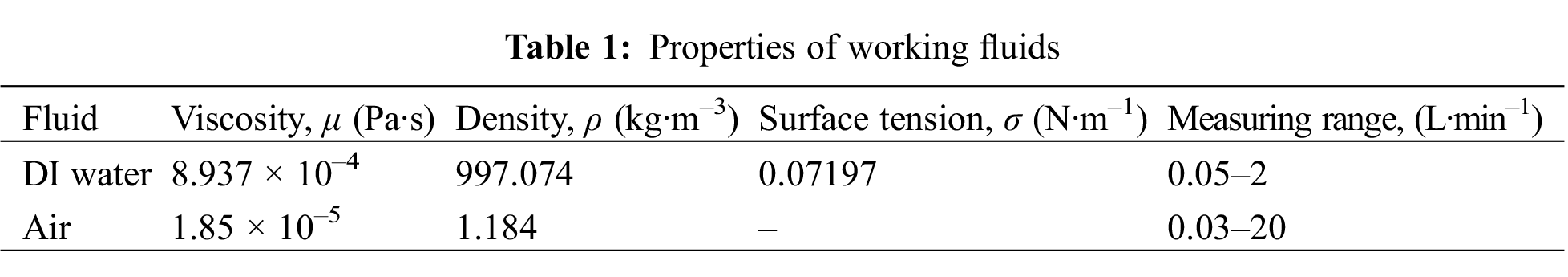
Fig. 1 is a schematic diagram of the experimental facility. The experimental apparatus mainly includes four parts: water supply system, gas supply system, experimental section and data acquisition system. The circulating power of the water circuit is supplied by a gear pump. After the continuous phase (DI water) flows through the gear pump, it enters the mass flow meter, flows into the visualization experiment section, and finally flows into the water tank to complete the water circulation. The power of the gas circuit is supplied by an air compressor and stored by a fixed large gas storage tank. The gas passes through an air filter and a pressure reducing valve, and gas flow meters of different ranges are selected according to the experimental conditions, and then enters the experimental section through a one-way valve to complete the gas circuit cycle. Water circulation power is provided by two types of miniature magnetic pumps. The range of the MG204XK miniature magnetic pump is 20–1000 ml/min, and the range of the MG209XK model is 100–2500 ml/min. The liquid flowmeter adopts the CX-CMFI Coriolis flowmeter of model DN6, the maximum measuring range is 700 kg/h, and the accuracy grade is ±0.2%. The power of the gas path is supplied by an Outstanding air compressor, with a maximum working pressure of 30 MPA. The air compressor has a power of 4500 W, a displacement of 420 L/min, and a tank capacity of 100 L. To reduce the experimental error caused by the unstable air pressure during the experiment, a 300 L fixed large gas storage tank is connected behind the air compressor to provide power for the experimental section. The rated pressure of the air storage tank is 0.7 MPA. When the compressed air in the air storage tank is less than 0.4 MPA during the experiment, the air compressor will automatically start to increase the air pressure in the air storage tank to 0.7 MPA to ensure the stability of gas flow rate and pressure before entering the experimental section.

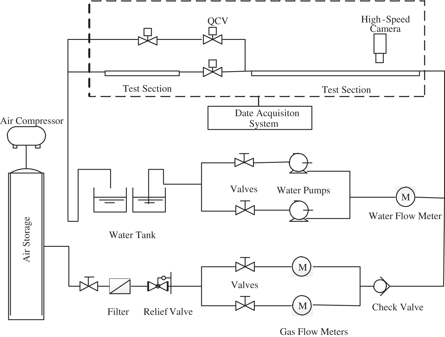
Figure 1: Schematic diagram of the experimental facility

To obtain more accurate experimental data, the filtered air enters the experimental section through two Sevenstar gas mass flow controllers with different ranges. Two types of gas mass flow controller models are D07-9E (range 0–50 L/min) and D07-19B (range 0–2 L/min).

The experimental section uses a quartz glass tube with good light transmission, and the length of the experimental section is 2000 mm in total. As shown in Fig. 2, the experimental section is divided into two parts, namely the flow pattern capture unit and the void fraction calibration unit.

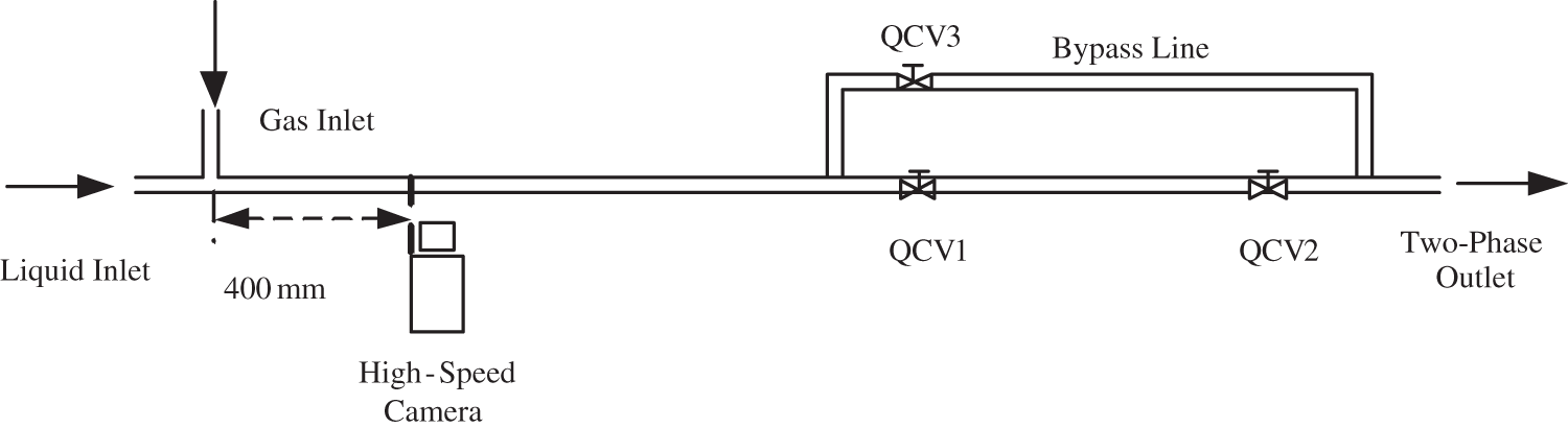
Figure 2: Schematic diagram of the test section

The front part of the experimental section is a flow pattern capture unit. The camera model used in this paper is Photron nova s6. In the experimental test, the recording rate of the high-speed camera is 1000 frames per second and the resolution is 2560 × 1920 pixels. All digital data has been stored in the computer. To distribute the light source evenly and improve the image quality, the light source of the experimental section uses two identical LED backlighting and uses green sulfuric acid paper to evenly cover the lamp body. The void fraction calibration unit is composed of three synchronous solenoid valves, a calibration tube and a high-precision electronic scale. The three synchronous solenoid valves are two normally closed solenoid valves with two-position and two-way and one normally open solenoid valve with two-position and two-way. The high-precision electronic scale has a range of 0–1000 g and an accuracy of 0.01 g.

Normally closed solenoid valves are installed at the front and rear ends of the calibration tube. Meanwhile, a branch is installed at the front end of the calibration tube and a normally open solenoid valve is installed on the branch. The flow pattern runs stably under a certain working condition, the power supply and the normally closed solenoid valve are opened, and the two-phase fluid passes through the calibration tube. When the flow pattern in the calibration tube is stable, the power is cut off, the normally open solenoid valve is opened, and the two-phase fluid flows back into the water tank from the branch. The instantaneous volume parameters of the two-phase fluid are retained in the calibration tube. In previous studies, the liquid in the calibration tube is generally poured out for weighing, but the inner diameter of the small pipe is small, and the liquid volume is small. If the liquid in the calibration tube is directly calibrated, the slight remaining liquid in the calibration tube has a greater impact on the void fraction, so this paper adopts the method of directly weighing the calibration tube.

It is necessary to weigh the calibration tube before the calibration experiment. The mass of the calibration tube is M1, and the calibration tube is M2 when it is filled with DI water. Therefore, the quality (Mfull) of water when the entire calibration tube is filled with water can be determined:

Mfull=M2−M1 (1)

To obtain a more accurate void fraction under a certain working condition, at least five calibration experiments need to be repeated for each working condition. Assuming that the mass of the calibration tube is Mti during calibration, the mass of the calibration tube under a certain working condition is Mt:

Mt=∑i=15Mti (2)

Ignore the air quality, the quality of water in the calibration tube Mw:

Mw=Mt−M1 (3)

The volume of the calibration tube is set to V, the volume of the gas and liquid phases are respectively Vg and Vl, and the density of the liquid phase is ρl, then the volumetric void fraction in the calibration tube under a certain working condition is α:

α=VgV=1−VlV=1−MwρlρlMfull=1−MwMfull (4)

3  Results and Discussion

3.1 Flow Regime Maps

Fig. 3 shows the flow regime maps and the transition boundary curves between different flow patterns. The flow patterns in horizontal tubes have been recognized as bubble flow, slug flow, annular flow, stratified flow, etc. Compared with the 6 mm horizontal circular pipe flow pattern transition boundary researched by Barnea and the theoretical transition boundary of Taitel & Dukler, the flow pattern transition boundary curves of stratified flow and annular flow are in good agreement with the Barnea curve. As the pipe diameter decreases, the transition boundary between bubbly flow and slug flow occurs at a slightly higher gas phase velocity. The Taitel & Dukler theoretical model does not consider the influence of surface tension on the transition boundary between stratified flow and slug flow. Therefore, the boundary line of Taitel & Dukler slug flow and stratified flow appears at a higher liquid phase conversion velocity than in this paper.

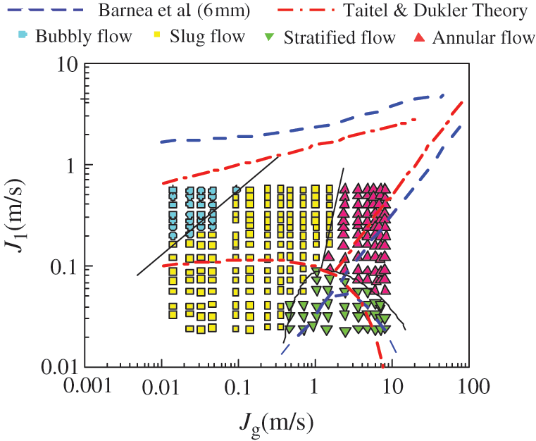
Figure 3: Flow regime map in gas-liquid two-phase flow

3.2 Void Fraction

To verify the accuracy of the image processing and calculation of the void fraction, the quick closing valve (QCV) is used to measure the void fraction. Fig. 4 shows that the error between the experimental and calculated volumetric void fraction is less than 10%, which shows that the calculation of void fraction t based on image processing is feasible.

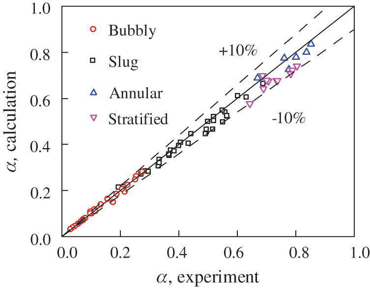
Figure 4: Comparison of volumetric void fraction between experimental and calculated results

Fig. 5 shows the instantaneous cross-sectional void fraction images of four different flow patterns with time in a 6.68 mm pipe diameter. The cross-section void fraction γ refers to the percentage of the area occupied by the gas phase on a certain cross-section in an instantaneous state. Fig. 5(a) is a schematic diagram of the void fraction of the bubbly flow section changing with time. The front and back of the bubble in the bubbly flow are more uniform, the cross-sectional void fraction peak is in the middle of the bubble, and the cross-sectional void fraction before and after the bubble decreases uniformly. From the figure, the length ratio between the bubble and the liquid slug and the frequency of bubble appearance is observed. Fig. 5(b) is a schematic diagram of the void fraction of the slug flow section changing with time. It can be seen that the distribution of the gas slug is not uniform, and the cross-sectional void fraction peak is shifted to the tail of the gas slug, but a clear peak can still be seen. Compared with the bubbly flow, the peak of slug flow is higher, and its waist is wider. Fig. 5(c) is a schematic diagram of the void fraction of a typical annular flow section changing with time. Because the annular flow is continuous, the cross-sectional void fraction image does not have obvious peaks like intermittent flows (bubbly flow and slug flow), instead, it keeps fluctuating at a higher cross-sectional gas content, and its fluctuation amplitude is larger. Under normal circumstances, as the gas flow rate increases, the degree of chaos in the cross-section of the annular flow gas-liquid phase increases, and the fluctuation range of the cross-section void fraction will be more severe. Fig. 5(d) is a schematic diagram of the change of the void fraction of the stratified flow section with time. Compared with the annular flow, the void fraction of the stratified flow section fluctuates more gently, and the fluctuation range is mostly maintained at γ = 0.6. With the increase or decrease of the gas flow rate, the cross-section void fraction image will also show a trend of increased and smoother fluctuations.

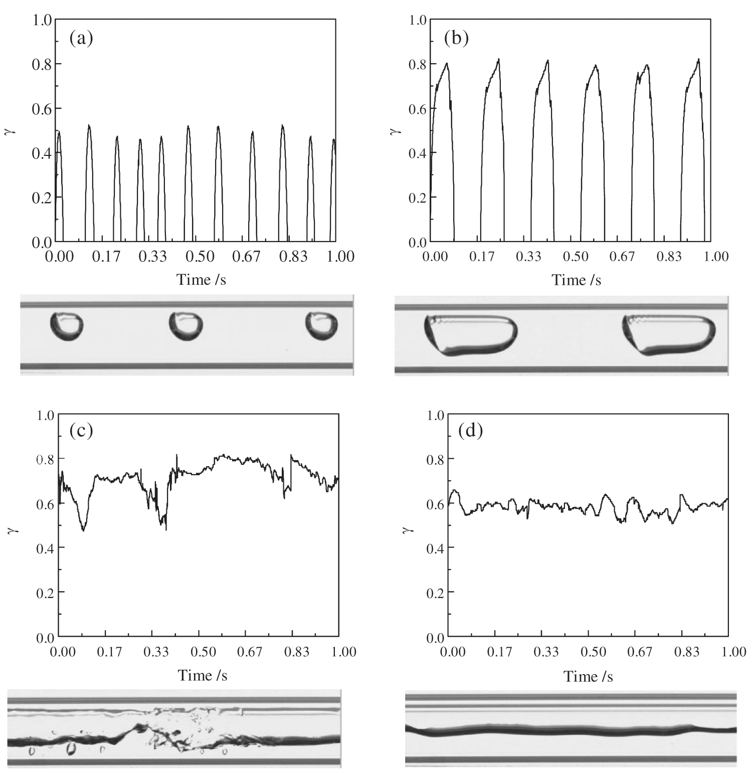
Figure 5: The cross-sectional void fraction of different flow patterns. (a) Bubbly flow, (b) Slug flow, (c) Annular flow, (d) Stratified flow

Probability distribution function (PDF) is a statistical function that describes all the possible values and likelihoods that a random variable can take within a given range. Fig. 6 is a PDF image of the cross-sectional void fraction of different flow patterns. Bubbly flow and slug flow are intermittent flow, and gas-liquid phases appear alternately. Therefore, the PDF images of slug and bubbly flow have a bimodal structure. The peak at the zero point represents the total time domain of the entire liquid phase (called the liquid phase peak), and the other peak represents the total time domain of the bubble flowing through a certain section (called the gas phase peak). In the bubbly flow, because the bubbles occupy less section of the pipe and the liquid slug occupies the main area of the pipe, the peak value of the liquid phase of the bubbly flow in the three pipe diameters is higher, instead, the gas phase peak is relatively flat and the peak value is extremely low. As the gas flow rate increases, the gas phase occupying the pipeline area increases, the gas phase peak rises and forms an obvious peak, while the liquid phase peak value drops, and the flow pattern changes to slug flow at a certain moment. Since the continuous gas-liquid flow is not intermittent, annular flow and stratified flow are unimodal. The gas-liquid velocity of the stratified flow is relatively low, the phase interface is relatively flat, and the fluctuation range of the cross-sectional void fraction is small. Therefore, the single peak of the cross-sectional void fraction PDF image of the stratified flow is more prominent, while the single peak of the annular flow is lower. The peak waist is also wider than the stratified flow.

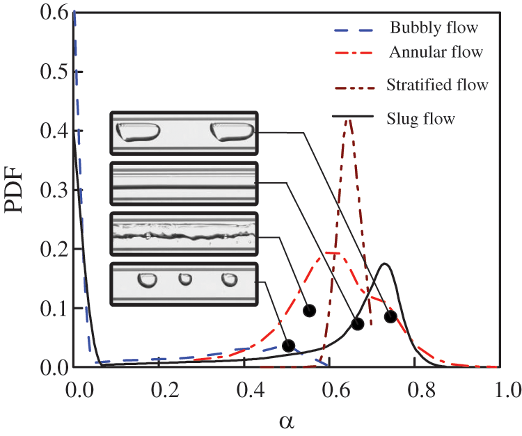
Figure 6: Probability distribution function (PDF) of void fraction data for different flow patterns

3.3 Evaluation of the Void Fraction Model

As described earlier, the accurate prediction of the void fraction is also crucial. This paper selects four different prediction models: slip rate structure model (Smith model); KαH structure model (Chisholm model); drift flux structure model (Gregory-Scott model) and a set of empirical formula structure models (Huq-Loth model). In order to evaluate the correlation of the four groups of void fractions, this paper introduces the absolute error (MAD, mean absolute relative deviation), root mean square error (RMSE) and cut-off parameter (NUM) to evaluate the void fraction model, which is used to predict the accuracy of the void fraction data in this paper. The absolute error (MAD) is the evaluation of the fluctuation amplitude of the error distribution, and the root mean square error (RMSE) is the evaluation of the dispersion of the prediction error of the void fraction model. Combining the two can comprehensively evaluate the predictive ability of a certain void fraction model to the experimental data points, and then can initially screen out the void fraction model that can more accurately predict the void fraction data in this paper. In order to better evaluate the ability of the void fraction model to predict the experimental data of the void fraction in this paper, the most accurate prediction model is selected. In this paper, cut-off parameters (NUM) are used to judge the evaluation ability of the model within a certain cut-off range to determine whether the model is good. Two cut-off errors of 10% and 25% are used as the evaluation parameters in this paper. The cut-off parameter (NUM) is defined as the ratio of the number of void fraction less than the cut-off error in the model prediction to the total predicted void fraction.

MAD=1M∑λ=1M|y(λ)pred−y(λ)expy(λ)exp|×100% (5)

RMSE=1M∑λ=1M(y(λ)pred−y(λ)expy(λ)exp)2×100% (6)

NUM1=1Msumif(|y(λ)pred−y(λ)expy(λ)exp|≤0.10)×100% (7)

NUM2=1Msumif(|y(λ)pred−y(λ)expy(λ)exp|≤0.25)×100% (8)

sumif is a function to solve the total number of parameters that meet the conditions. y(λ)pred and y(λ)exp are the predicted and experimental values of the λth data point, respectively, and M is the number of experimental data points.

Tab. 2 is the evaluation parameter table of the four groups of prediction models. As shown in Fig. 7, from the MAD and RMSE evaluation parameters alone, the four void fraction formulas can above predict the void fraction well. When the cut-off error is 10%, all the prediction effects of the void fraction model are lower than 55%. But when the cut-off error is 25%, the prediction effect of all models is significantly improved to about 95%.

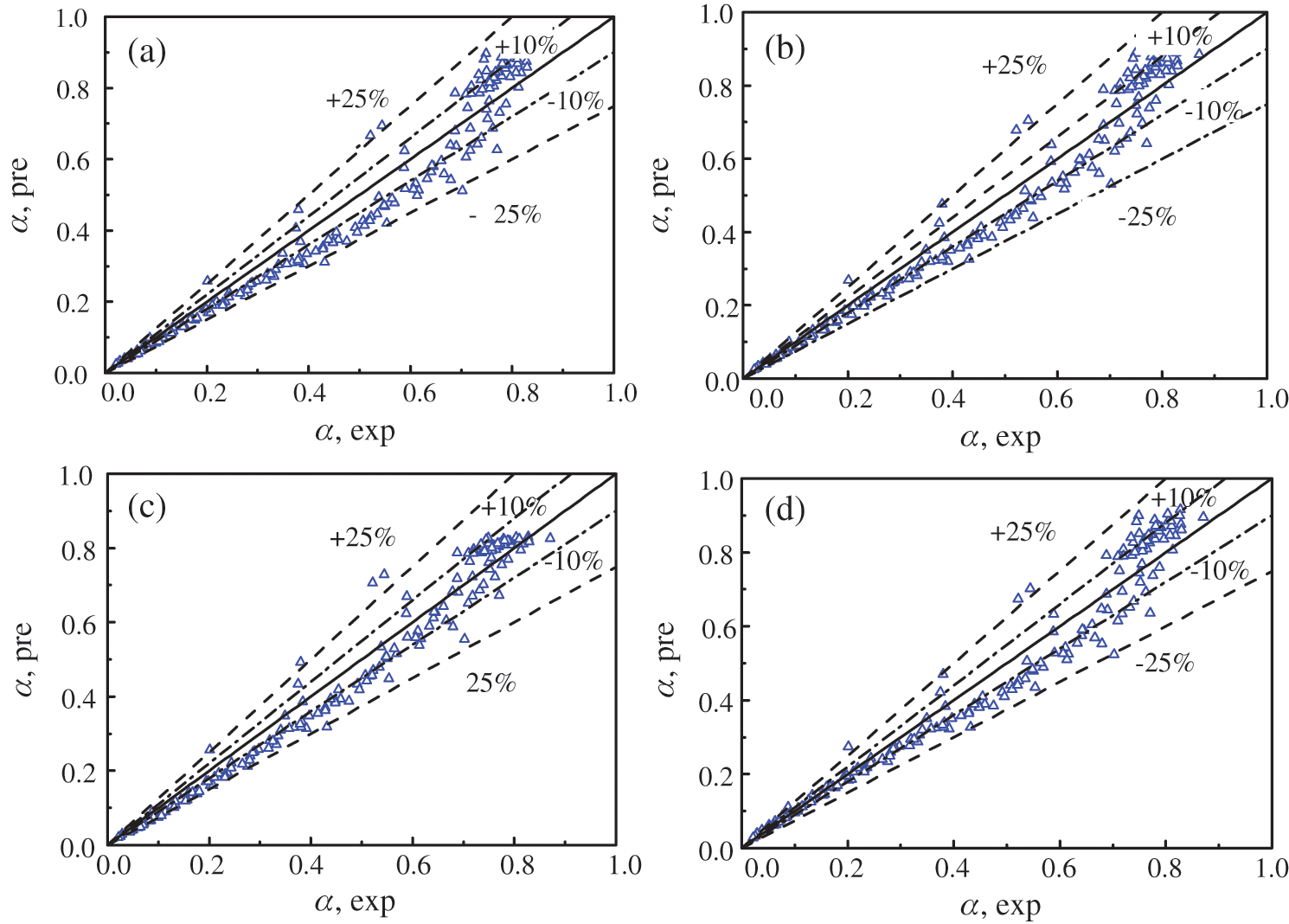
Figure 7: Comparison of the experimental results and predicted data. (a) Smith model, (b) Chishlom model, (c) Gregory-Scott model, (d) Huq-Loth model

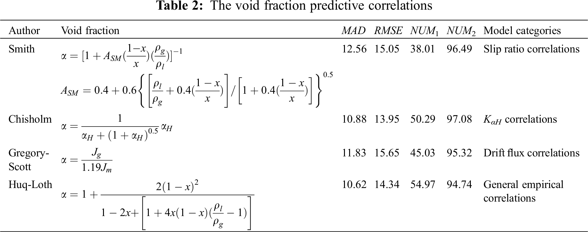
It can be seen from the table that the Chisholm void fraction prediction model has better fitting results than other models. From the table, it can be found that the Gregory-Scott void fraction prediction model has a small data gap with the Chisholm void fraction prediction model. At the same time, considering that the drift flux structure is more advanced than other structures, it is considered based on the drift flux structure to improve the void fraction prediction model. In order to simplify the complexity of the prediction model, the local relative flow between phases is ignored when the void fraction prediction model is fitted. The experimental results prove that this method has little effect on the void fraction prediction performance. Fig. 8 shows the trend curve of β/α with the change of dryness. β is the ratio of the gas-phase volume flow rate to the total gas-liquid two-phase volume flow rate. It can be seen from the figure that when the dryness is at a small level (x < 0.01), the value of β/α almost all falls in the area less than 1.19, which is located below the curve of the Gregory-Scott model. As the dryness increases, the value of β/α gradually increases, and the number of positions falling on β/α > 1.19 gradually increases. Therefore, the relationship between β/α and the void fraction should be a curve with a smaller slope. It can be explained that as the void fraction increases, the velocity of the void fraction increases, and the liquid phase is affected by friction and virtual mass force during the movement. Compared with the rate of β increase, the rate of increase of the void fraction α will slow down. In summary, this paper is based on the Gregory-Scott model to improve, and defines the void fraction as one of the influencing factors of C0. Considering that the dryness affects the cross-section void fraction, a correction factor (x1−x)k is added to the C0 position of the prediction model. Jg is the converted velocity of the gas phase, and Jm is the converted velocity difference between the liquid phase and the gas phase. α is the volumetric void fraction of the calibration tube. x is the mass void fraction (the dryness) measured in the calibration tube. At the same time, considering the effect of surface tension, the surface tension coefficient σ is introduced. After many experiments, the above experimental parameters are brought into the fitting formula, and through numerical fitting, the revised Gregory model is finally obtained:

α=Jg1.4(x1−x)σ1.852Jm (9)

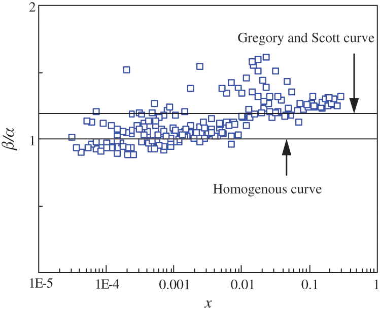
Figure 8: Variation of β/α with change in x

The modified Gregory-Scott model was used to fit the void fraction data, and the results are shown in Fig. 9. Tab. 3 is the performance evaluation table of the improved model. In order to compare the optimization degree of the improved formula relative to the Gregory prediction model, the optimization degree ψ is introduced to evaluate the optimization degree as a whole. The optimization degree ψ is defined as the ratio of the difference between the predicted parameter k of the Gregory-Scott model (including MAD, RMSE, NUM1, NUM2, etc.) and the predicted parameter k’ of the improved model to the predicted parameter k of the Gregory-Scott model.

ψ=k′−kk (10)

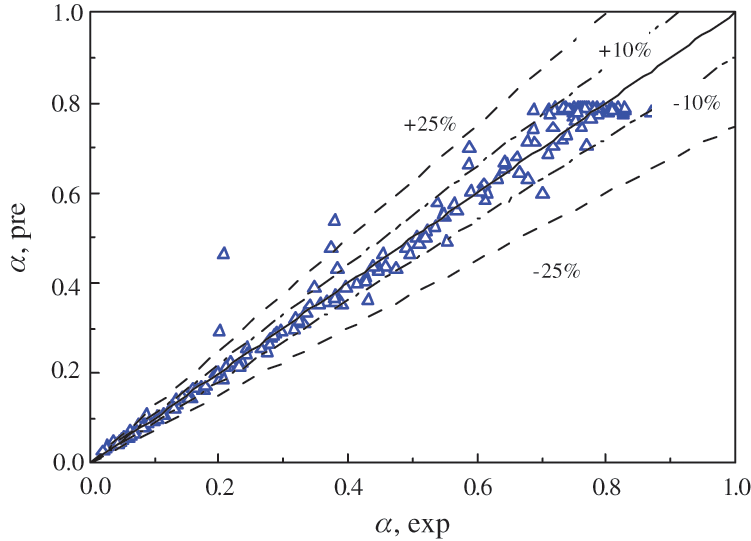
Figure 9: Comparison of the improved void fraction correlation with experimental data

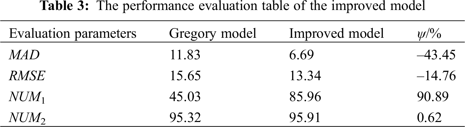
It can be seen from the table that compared with the Gregory-Scott model, the improved model has significantly improved the predictive ability of the void fraction in this paper. This improvement is reflected in the decrease of 43.45% in absolute error optimization and 14.76% in root mean square error. This shows that the fluctuation amplitude of the error distribution is greatly reduced, and the prediction errors of the void fraction model are more concentrated. The optimization degree of the cut-off parameters under the cut-off error NUM1 is 90.89%, and the optimization effect is obvious. In summary, the improved model proposed in this paper is feasible and effective.

4  Conclusion

This paper studies the gas-liquid two-phase flow in a horizontal circular tube with an inner diameter of 6.68 mm. The flow pattern is captured by a high-speed camera. The void fraction of the four flow patterns is calculated using image processing technology and verified by a quick closing valve. Analyzed the characteristics of the cross-section void fraction of various flow patterns, and evaluated four typical void fraction prediction models, and obtained the following main conclusions:

1.    The experiment observed that the main flow patterns in the horizontal circular channel are bubbly flow, slug flow, annular flow and stratified flow. Compared with conventional channels, the gravity effect in the small channel is weakened, the surface tension is strengthened, the annular flow occupies a relatively large proportion on the flow regime map, and the stratified flow occupies a small proportion.

2.    It is found that the intermittent flow (bubbly flow, slug flow) has a knife-edge cross-sectional void fraction, and the PDF image of the cross-sectional void fraction is a bimodal structure; The cross-sectional void fraction of continuous flow (annular flow, stratified flow) is a fluctuating continuous curve, and the PDF image of the cross-sectional void fraction is a unimodal structure.

3.    The experiment also compares the volumetric void fraction with the four sets of void fraction formulas. The results show that the four model structures can predict the void fraction data in this paper very well. The void fraction prediction model is improved for the Gregory and Scott model, which significantly improves the prediction accuracy.

Funding Statement: This work was supported by the Guangdong Basic and Applied Basic Research Foundation (2019A1515111116), Key R&D Program of Shandong Province (Nos. 2019GSF109051, 2019GGX101030), Shandong Provincial Postdoctoral Innovation Project (No. 201902002), and Foundation of Shandong University for Young Scholar’s Future Plans.

Conflicts of Interest: The authors declare that they have no conflicts of interest to report regarding the present study.

This work is licensed under a Creative Commons Attribution 4.0 International License, which permits unrestricted use, distribution, and reproduction in any medium, provided the original work is properly cited.