Fluid Dynamics & Materials Processing

DOI: 10.32604/fdmp.2022.017869

ARTICLE

Numerical Simulation of Wake Vortices Generated by an A330-200 Aircraft in the Nearfield Phase

Xuan Wang and Weijun Pan*

College of Air Traffic Management, Civil Aviation Flight University of China, Deyang, China
*Corresponding Author: Weijun Pan. Email: atcxaun@cafuc.edu.cn
Received: 13 June 2021; Accepted: 18 September 2021

1  Introduction

Lift causes strong, steady and spatially extensive wake vortices to be generated by an aircraft. An aircraft is accident-prone in the approach phase due to strong long-lasting wake vortices of the preceding aircraft [1,2]. To deal with this issue, the aircraft wake separations during the takeoff and landing phases are specified by the International Civil Aviation Organization (ICAO) and the Civil Aviation Administration of China (CACC) [3]. However, the wake separation cannot be defined rigorously because different types of aircraft have different wake vortex intensities generated by themselves and in their capacity to withstand those exerted by the preceding aircraft. A large margin is given in current wake separation standards in order to ensure safety. However, an excessively large wake separation may affect the takeoff and landing efficiency. Therefore, accurate prediction of the aircraft wake structure in the approach phase has always been a key focus in the civil aviation sector [4,5].

Along with the development in computer technologies, local and international researchers have extensively studied wake vortices by using the computational fluid dynamics (CFD) approach since the 1970s. Crow [6] studied the optimal instability mode of a mutually-induced vortex pair based on the first-order model of the Biot-Savart Law. The author pointed out that the long-wave instability was one of the reasons for rapid decay of wake vortices. Corjon et al. [7] optimized the wake vortex estimation model by including the near-surface wind and crosswind effects. Stephan et al. [8] simplified the model for wake vortices in the approach phase and neglected the effects of wake vortices generated at different altitudes and during landing. Nybelen et al. [9] simulated the merging process of wake vortex systems and their instability via direct numerical simulations and large eddy simulations (LES).

Misaka et al. [10] studied the dynamic process from generation to dissipation of wake vortexes under turbulence, thermal stability, wind shear, and other atmospheric conditions based on the LES. As the hybrid RANS/LES model developed in recent years, Holzäpfel et al. [11,12] studied the effects of the crosswind and ground obstacle on the dissipation of wake vortices based on the simulations of realistic complex wake structures in the nearfield phase. In 2016, Stuart et al. [13] established a numerical model for a separate trailing vortex and wall surface, and further studied its linear optimal initial perturbation. Paramasivam et al. [14] used the LES to explore the effects of crosswind and atmospheric turbulence on the dissipation of wake vortices. Misaka et al. [15] numerically simulated the jet-wake vortex interaction in the nearfield and extended nearfield phases. scholars such as Lin et al. [16] also studied wake vortices based on numerical simulations. A method of producing wake vortices on the lift surface was proposed to study the evolution characteristics of aircraft wake vortices in the atmosphere, and a fast wake prediction system was established based on the method.

Computational fluid dynamics is a new interdisciplinary subject that integrates fluid mechanics and computer science. It is applied in several fields such as medical care, aviation, and high-speed rail [17–20]. Currently, most numerical simulations of aircraft wake vortices are based on a simplified rectangular wing. The effects of wake vortices on the fuselage structure, sweepback angle and cross-sectional variation of wings, and horizontal and vertical tails are rarely verified, and wake vortices under crosswind conditions are infrequently simulated. For all these reasons, we select the A330-200 aircraft as the study object, which is an internationally used aircraft. We use Pointwise for grid meshing of this aircraft, and utilize the ANSYS FLUENT to numerically simulate the flow field of the whole aircraft in the final approach segment and the flow field under crosswind conditions. We obtain the evolution characteristics of wake vortices of the A330-200 aircraft in the final approach phase by using Tecplot for post-processing of simulated flow field structure, which provide theoretical support for reduced wake separation of this type of aircraft.

2  Computational Model and Numerical Simulation-Based Research of Aircraft Wake Vortices in Nearfield Phase

The fluid motion abides by the three major conservation laws in physics: law of conservation of mass, law of conservation of momentum, and law of conservation of energy. The mathematical description of the fluid motion process constrained and restricted by these three laws constitutes the Navier-Stokes equations. In this paper, the governing equation, spatial discrete method, turbulence model and limiter used in numerical simulation have been extensively verified.

Regardless of the volume force and the external heat source, the differential form of the three-dimensional unsteady compressible Navier-Stokes equation with respect to the conserved variable in the Cartesian coordinate system can be written as:

∂Q∂t+∂F∂x+∂G∂y+∂H∂z=∂Fν∂x+∂Gν∂y+∂Hν∂z (1)

where F, G and H are the inviscid vector flux of the convection term, Fv, Gv and Hv are the viscous vector flux, the specific form is:

Q=(ρρuρvρwρe),F=(ρuρu2+pρuvρuw(ρe+p)u),G=(ρvρuvρv2+pρvw(ρe+p)v),H=(ρwρuwρvwρw2+p(ρe+p)w)Fν=(0τxxτxyτxzφx),Gν=(0τyxτyyτyzφy),Hν=(0τzxτzyτzzφz) (2)

In the above formula,

φx=uτxx+vτxy+wτxz−qxφy=uτyx+vτyy+wτyz−qyφz=uτzx+vτzy+wτzz−qz (3)

where, ρ is the fluid density, u,v,w is the velocity component in Cartesian coordinate system, p is the fluid pressure, and e is the total energy per unit mass of gas. The specific formula is as follows:

e=1γ−1pρ+12(u2+v2+w2) (4)

In the formula, the viscous stress term is:

τxx=23μ(2∂u∂x−∂v∂y−∂w∂z);τxy=τyx=μ(∂u∂y+∂v∂x)τyy=23μ(2∂v∂y−∂u∂x−∂w∂z);τyz=τzy=μ(∂v∂z+∂w∂y)τzz=23μ(2∂w∂z−∂u∂x−∂v∂y);τzx=τxz=μ(∂w∂x+∂u∂z) (5)

Heat flux is:

qx=−μ(γ−1)Pr∂T∂xqy=−μ(γ−1)Pr∂T∂yqz=−μ(γ−1)Pr∂T∂z (6)

The discretized calculation of viscosity terms involved in the solution of the Navier-Stokes equations is usually complicated, resulting in a long calculation time and low efficiency. In the actual flow, compared with the viscosity terms perpendicular to the main flow direction, the viscous terms in the main flow direction and the interaction between them are mostly very weak.

Several studies show that the viscous effect is significant only near the solid walls for high Reynolds number flows without a large separation. Compared with the viscous terms along the normal direction of the object surface, those along its tangential direction are very small, which, therefore, appear unimportant. The dimensional analysis shows that the viscous terms in the tangential direction of the object surface can be ignored. Therefore, a thin-layer approximation hypothesis is proposed based on the two perspectives of physics and computations. According to the hypothesis, only the viscous terms along the normal direction of the object surface in the governing equation are retained. The thin-layer hypothesis is the simplification of Navier-Stokes equations, which is widely applied and coincides well with experimental data. At present, compressible thin-layer Navier-Stokes equations are widely applied in most three-dimensional viscous flow calculations, which can significantly improve computational efficiency and simplify the program composition.

In this way, the viscous flux term in the Navier-Stokes equations with the thin-layer hypothesis can be simplified as

F^ν=μJ(0ϕ1uξ+ξxϕ2ϕ1vξ+ξyϕ2ϕ1wξ+ξzϕ2ϕ1(ϕ3+εTξ)+ϕ2(U−ξt));{ϕ1=ξx2+ξy2+ξz2ϕ2=13(uξξx+vξξy+wξξz)ϕ3=uuξ+vvξ+wwξG^ν=μJ(0θ1uη+ηxθ2θ1vη+ηyθ2θ1wη+ηzθ2θ1(θ3+εTη)+θ2(V−ηt));{θ1=ηx2+ηy2+ηz2θ2=13(uηηx+vηηy+wηηz)θ3=uuη+vvη+wwηH^ν=μJ(0φ1uζ+ζxφ2φ1vζ+ζyφ2φ1wζ+ζzφ2φ1(φ3+εTζ)+φ2(W−ζt));{φ1=ζx2+ζy2+ζz2φ2=13(uζζx+vζζy+wζζz)φ3=uuζ+vvζ+wwζ (7)

In this paper, the most widely applied two-equation vortex-viscosity Wilcox k−ω model is selected as the turbulence model. This model is a two-equation vortex-viscosity model for incompressible and compressible turbulence integrated to the wall surface, which is mainly used to solve the convey-diffuse equation for turbulent kinetic energy k and its specific dissipation rate.

The vortex-viscosity model of Reynolds stress is:

τtij=2μt(Sij−Snnδij/3)−2ρkδij/3 (8)

In the formula, μt is the vortex-viscosity, Sij is the average velocity strain rate tensor, ρ is the fluid density, k is the turbulent kinetic energy, and δij is the Kronecker operator. Vortex-viscosity is defined as a function of turbulent kinetic energy k and specific dissipation rate ω , i.e.,

μt=ρk/ω (9)

The transport equation of k and ω are:

∂ρk∂t+∂∂xj[ρujk−(μ+σ∗μt)∂k∂xj]=τtijSij−β∗ρωk (10)

∂ρω∂t+∂∂xj[ρujω−(μ+σμt)∂ω∂xj]=αωkτtijSij−βρω2 (11)

2.1 Aircraft and Environmental Parameters

In this paper, the approach speed of the selected A330-200 aircraft assumed in this paper for numerical simulation of aircraft wake vortices in the approach phase is 100 m/s. As this speed is lower than 0.3 Mach, the fluid medium in the flow field is thus considered incompressible,Therefore, this paper selects the pressure-based solver for low-speed and incompressible fluid , rather than a density-based solver. The model used herein is drawn at a scale of 1:1 with respect to the A330-200 aircraft, which has a total length of 58.82 m, a wingspan of 60.30 m, and a maximum landing weight of 182,000 kg. The model only simplifies the engine profile, the engine jet, and the openings at flaps. Additionally, it includes the fuselage structure, sweepback angle and cross-sectional variation of wings, and horizontal and vertical tails compared with the conventional half-wing model. To describe typical takeoff and landing configurations, the angle of attack is considered as 7°. Table 1 provides the relevant parameters.

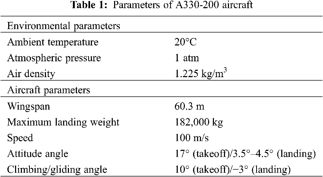
The computational model is established based on the wind tunnel flow field. The nose is considered as the origin of coordinates, 75 m extended up and down, 150 m left and right, 50 m in front and 500 m behind from the original. The overall dimensions are 550 m × 300 m× 150 m (L× W× H). The coordinate system is right-handed, with the x, y and z denoting the streamwise, spanwise and vertical directions, respectively. The aircraft wake structure within four times the wingspan can be simulated based on the length of the flow field.

Pointwise is used to draw grids of three parts. Fig. 1 shows the grid distribution and three-dimensional flow field structure. The area near the aircraft is partially encrypted. According to the calculation principle used in large vortex simulation, the vortex smaller than the smallest grid unit in the computation domain will be filtered out. Therefore, the grid size in the wake vortex region significantly influences the accuracy of the calculation results. Eight groups of grid cells with varying numbers are calculated to complete the grid independence test. Table 2 shows all the computational grids and computation results.

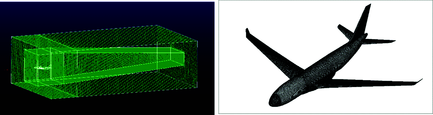
Figure 1: 3D flow field structure (left) and unstructured grids on wing surface (right)

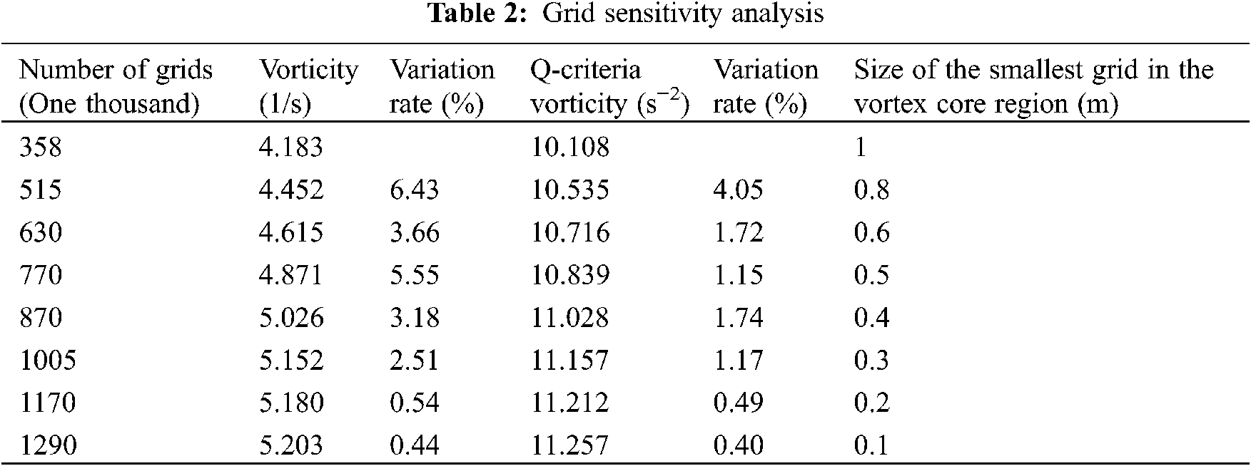
The selected vorticity and Q-criteria vorticity here are the maximum vorticity at the exit of the flow field, i.e., 500 m behind the wing unit. As the results show, once the number of grids reaches 12.9 million, the Q-criteria vorticity would change less as the number of grids increases. Furthermore, considering the computational time and resources, the first-layer grid is finally selected to be 1 cm high with a growth rate of 1.2, and the full-aircraft grids are obtained by filling after 25 times of growth. The number of grid nodes in the full aircraft is about 12.9 million, the flow field near the wake vortex is 100 W, and the ambient flow field is 450 W.

ANSYS Fluent is used for computational purpose, with the wall and inlet boundary set as the velocity inlet, approach speed of A330-200 aircraft as 100 m/s, and the outlet boundary as the pressure outlet. Furthermore, the average static pressure is considered as the standard atmospheric pressure of 1013.25 hPa, and the no-slip adiabatic solid wall-boundary is selected for the aircraft wall boundary. Based on the typical Reynolds number of 105 in the aviation sector and the inlet turbulence coefficient of 0.15%, the turbulivity of the flow field is suppressed in the rigid rotation region of the vortex core to improve the calculation of the average field in turbulent field.

2.2 Computational Model and Numerical Simulation Scheme of Aircraft Wake Vortices

To verify the effectiveness of the numerical simulation scheme, first, the semi-mode wing model of 1997 Chow’s near-field wingtip vortex was reduced by wing configuration of 1:1, with the half-width length being 3 feet, and the chord length being 4 feet. The wing configuration is NACA0012, and the angle of attack is 10°. Pointwise is used to draw the O-H flow field structure grids. Fig. 2 shows the flow field structure. The flow field height is 6 m with the trailing edge of the wing root taken as the coordinate origin, the front of the wing is 3 m, and the rear flow field is 4 m. Three times the chord length can be observed, with the marked as c. It is guaranteed that y + value is 1 to ensure the accuracy of the calculation results, and the height of the first layer grid is selected as 5e−7 m.

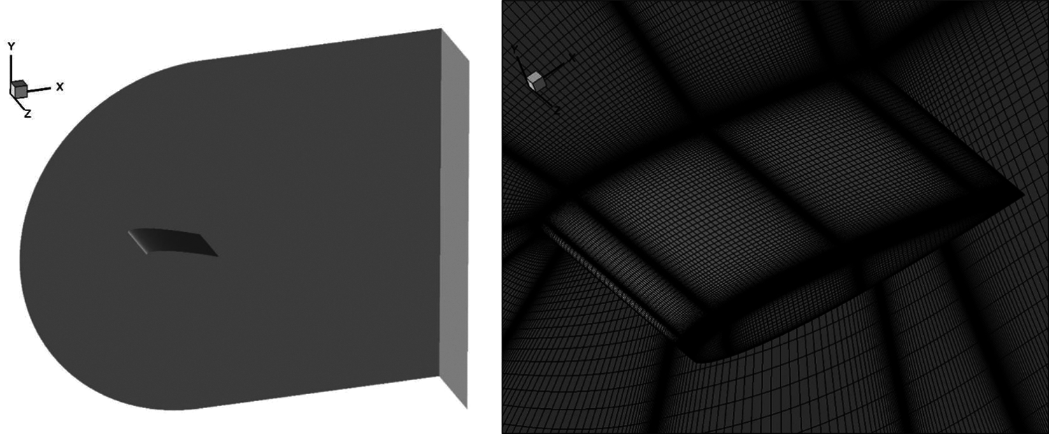
Figure 2: Smooth structure and division of grids near the wing

In numerical simulations, the incoming flow is selected as 170 ft/s, Reynolds number as 4.6 * 106, and turbulence coefficient as 0.15%. The results are all based on steady-state computation.

The accuracy of the numerical simulation model is verified by selecting the NASA’s standard calculation example for measuring the near-field wingtip vortex. In this paper, the verified SST-RC model [21] is used. This model is a modified version of the SST model with an empirical correction function added to limit the generation of turbulence energy. It is expressed in [22] as follows:

frotation=(1+cr1)2r∗1+r∗[1−cr3tan−1⁡(cr2r∼)]−cr1 (12)

where r∗ is the second-order gradient of velocity, r~ is the rotation of the system, cr1, cr2, cr3 represent empirical constants based on practical engineering applications, and frotation is limited between 0 and 1.25.

The steady flow is calculated using the pressure model-based scheme. The finite volume method (FVM) is used for discretization. Considering that the wake vortex are mostly rotating and swirling fluids, the accuracy of the results obtained by using the first-order scheme is poor. The second-order upwind scheme is used for pressure, momentum and energy equations as well as the turbulent dispersion. Fig. 3 compares the calculation results.

Figure 3: (a) Pressure coefficient distribution at 72.5% of wingtip (b) Experimental value for Chow pressure coefficient (c) Simulation value for Chow pressure coefficient

Fig. 3 compares the pressure coefficient distribution at 72.5% of wingspan and that in the flow field, respectively. It can be observed that the numerical simulation results accurately reflect the pressure distribution near the wing in the flow field. The error is controlled at 20%, and the error in multiple calculations is not more than 2%. The flow field structure is consistent with the actual case, indicating that the numerical simulation method can be used to predict the flow field near the wing.

Fig. 4 shows the flow chart used for numerical simulation of aircraft wake vortices, which can be implemented using the computational model and platform of wake vortices.

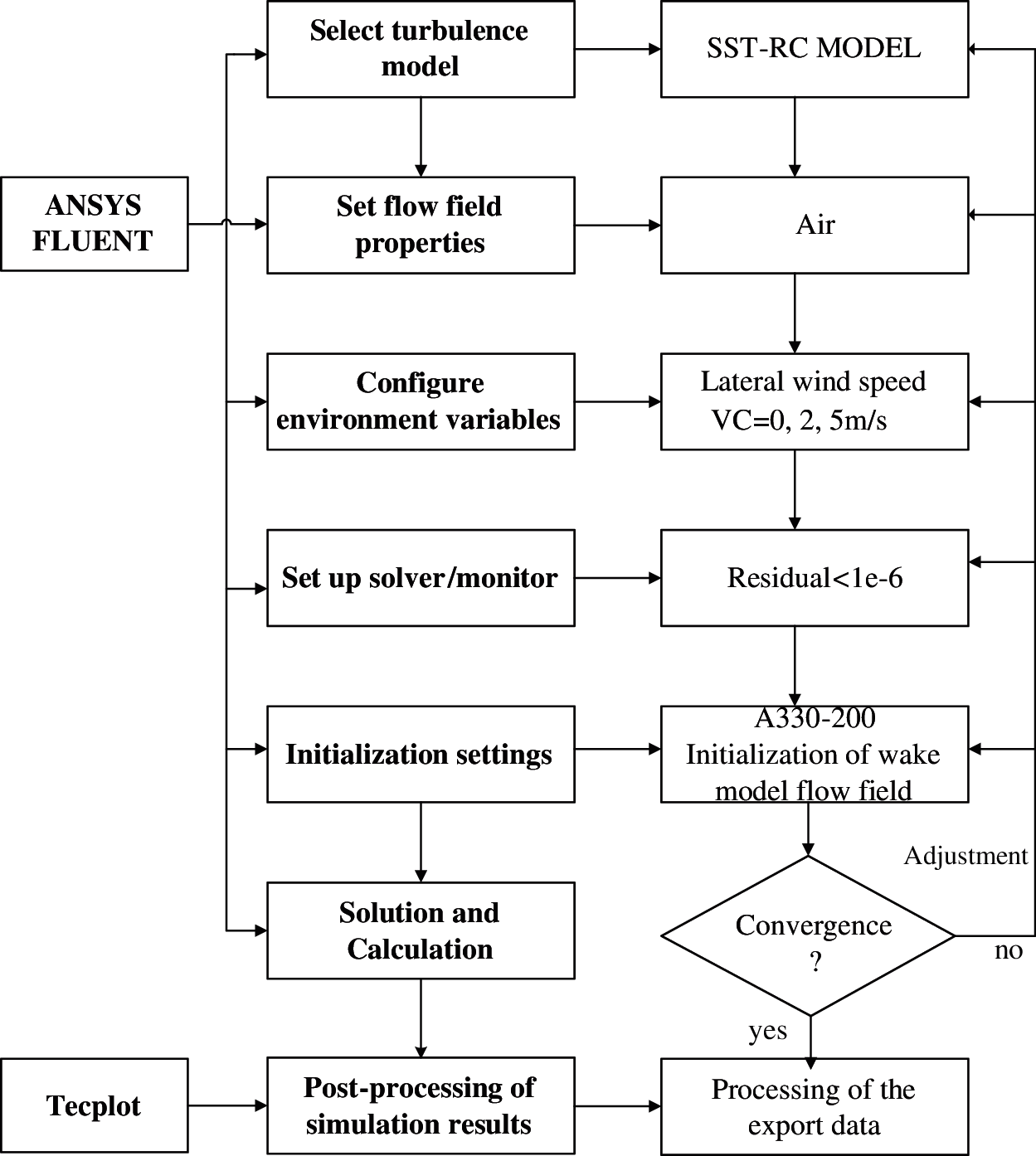
Figure 4: Flow chart for numerical simulation of aircraft wake vortices

3  Analysis of Evolution Characteristics of Aircraft Wake Vortices in Approach Phase under Calm Conditions

3.1 Wake Vortex Structure of Wing Flow Field

Fig. 5 shows the flow field structure on the upper surface of the leading edge for an A330-200 aircraft in a typical approach state. It can be observed that this structure differs significantly from the two-point structure in a traditional point vortex model. Four vortices in two symmetrically distributed pairs are formed after the air flows through the wing. Combined with the overall downwash effect, irregular turbulent vortex systems are finally generated in 3D space [23,24].

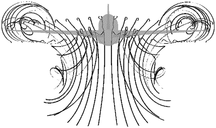
Figure 5: Streamline of upper surface of leading edge in a typical approach state

Fig. 6 shows the velocity contours in the XoZ plane at 20%, 40%, 60% and 80% of the wingspan. It can be observed that there is no flow separation in the flow field structure of 2D slices. In each section, the air flows through the upper and lower surfaces at higher and lower rates. The pressure difference between the two surfaces provides the necessary lift force. The velocity contours at 20% of the wingspan show that the horizontal tail also provides lift at this angle.

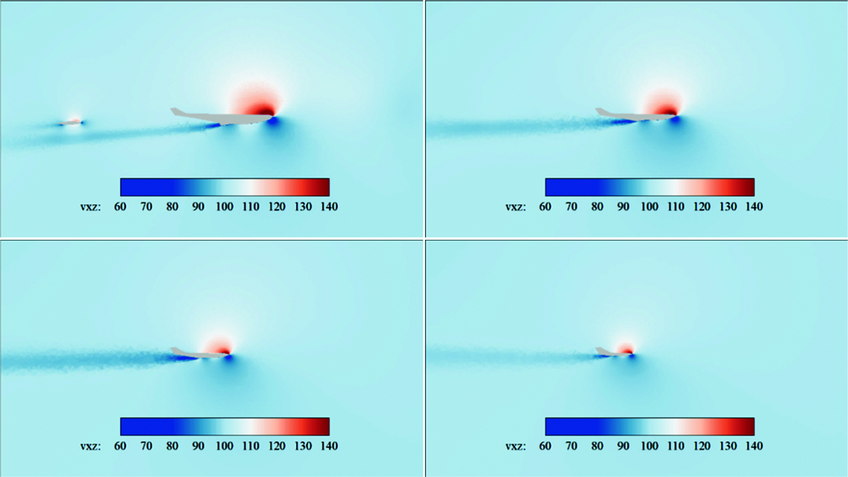
Figure 6: Velocity contours in XoZ plane at 20%, 40%, 60% and 80% of the wingspan

Fig. 7 shows the static pressure coefficient distribution over each wing section. It can be noted that due to significant pressure difference between the upper and lower surfaces of the wing tail, the rate of air on the upper wing surface increases when the air flows through the section tail, and the negative pressure increases. Due to the sweepback angle at a different wingspan section, the air on the lower surface close to the inner side rolls up towards the outer side while flowing backward. Consequently, some of the air flows in the plane perpendicular to the original flow direction. Superimposed with the stream wise velocity, spiral flow is eventually generated at the trailing edge [12,13].

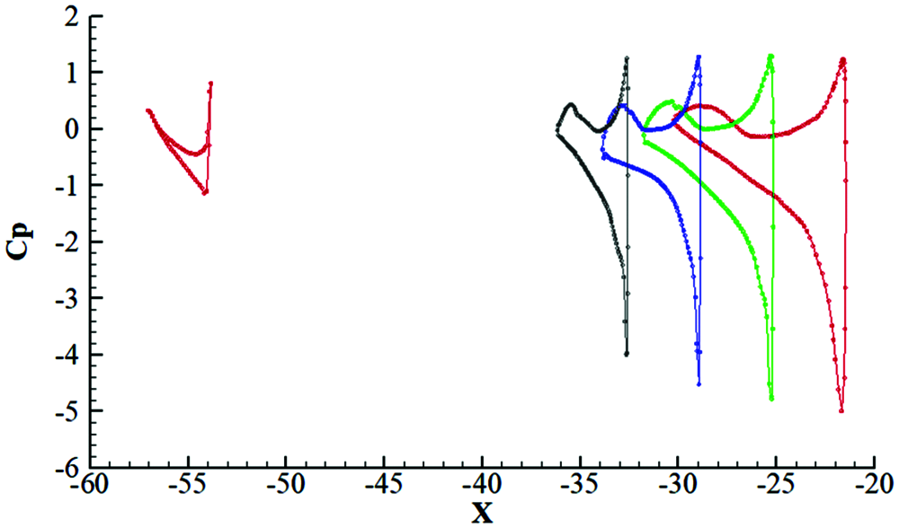
Figure 7: Cp distribution curve at 20%, 40%, 60% and 80% of the wingspan

3.2 Description of Wingtip Vortex Generation and Evolution Process

The slices at wingtip from X = −35 m to X = −39 m are selected. Fig. 8 shows the simulated contour of pressure distribution gradient. Sections are spaced 0.5 m apart. It can be observed from the figure that for the winglet structure of an A330-200 aircraft, the pressure transfers backward from the low-pressure area in the leading edge of the wingtip and splits into two directions when the air flows through the wing edge: one part of such pressure transfers obliquely backwards along the wingtip and the other part transfers obliquely upwards and backwards along the inner side of the winglet close to the outer edge. The pressure in the center of the low-pressure area is minimal at the leading edge. During the pressure transfer, the pressure in the center increases while the size of the center area gradually decreases. Two split streams of wingtip vortices are finally formed.

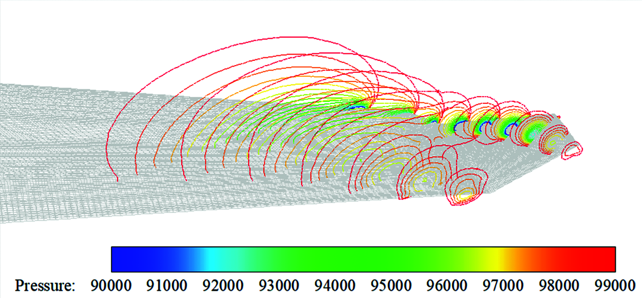
Figure 8: Contour of pressure distribution gradient for slices at wingtip from X = −35 m to X = −39 m

Fig. 9 shows the vorticity contour developed according to the Q criterion (Q = 7). It can be noted from the figure that there are separately-developed two streams of vortices: one at the physically bent structure of the wingtip, and the other at the inner outer edge of the winglet. The vortex core area gradually gets larger when wake vortices leave the wing structure. When sweeping backwards, wake vortices become increasingly closer and merge about 5 m behind the wingtip, forming a larger vortex core area. This is finally visualized as the two-part vortex system structure at the outer side in the four-vortex system, as shown in Fig. 10.

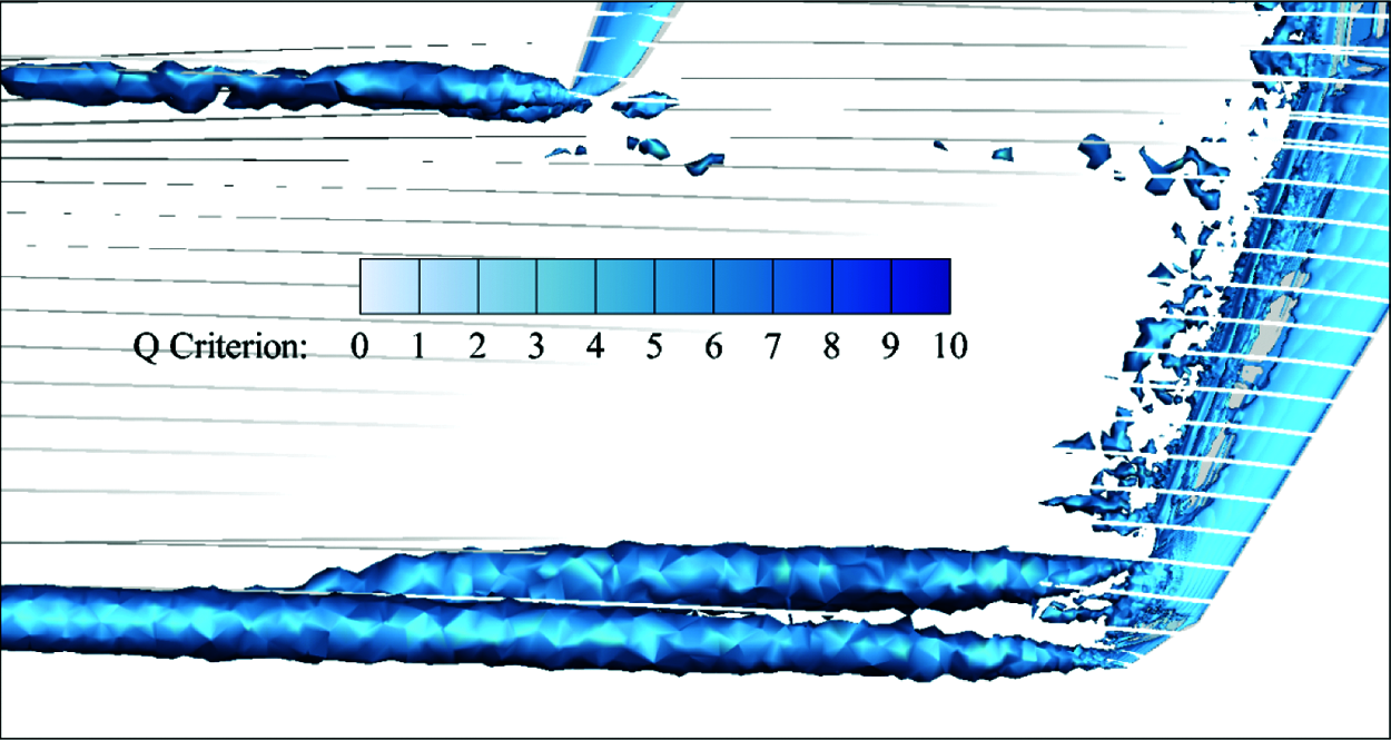
Figure 9: Vorticity contour (Q = 7)

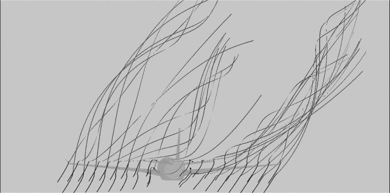
Figure 10: Streamline distribution over upper and lower wing surfaces

Fig. 11 shows the absolute vorticity in the X-axis direction at one to five times the wingspan, where the separation is 0.5 times the wingspan. It can be observed that as the flow field develops in its flow direction, the vorticity extremum in the X-axis direction slowly decreases, and the four-vortex system structure gradually rolls up inwards. The two vortex cores of the upper-half vortex system gradually move up and get closer to each other, while those of the lower-half vortex system gradually move down and get separated from each other. Finally, a point vortex mutually coupled by four parts is produced at a position corresponding to a distance of five times the wingspan.

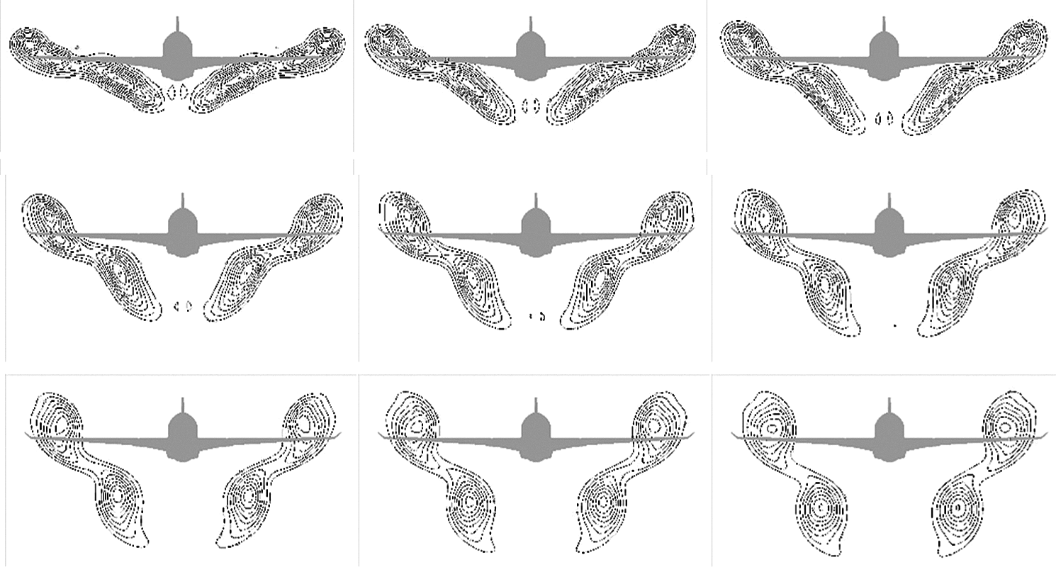
Figure 11: Absolute vorticity in X-axis direction at one to five times the wingspan

4  Analysis of Evolution Characteristics of Aircraft Wake Vortices in Approach Phase under Crosswind Conditions

The flow fields in the wind tunnel are simulated additionally under 2 m/s and 5 m/s crosswinds. The crosswinds are from the left side and vertical to the fuselage. The CFD simulations mainly emphasize the movement trend and the vorticity curve of the wing vortex system in the YOZ plane. Fig. 12 shows the vorticity curves of the wing wake vortices obtained under different crosswind conditions.

Figure 12: Vorticity curves of wake vortices under different crosswind conditions (Q criterion) (a) Vorticity comparison of wingtip vortices under Q criterion (b) Vorticity comparison of wing root vortices under Q criterion

The numbers marked horizontally in Fig. 10 indicate the wingspan length while those along the longitudinal axis represent the vorticity. The following points can be observed from the figure:

The wing wake vortices gradually dissipate over time to a lower level in the flow field.

The vorticity in the upstream of the crosswind is generally higher than that in the downstream.

The variations in vorticity of left and right wingtips show opposite trends due to crosswind effects as the wingtip vortices are eudipleural. These opposite trends mean that the vorticity increases at one side while that of the vortex system decreases on the other side.

At positions corresponding to a distance not less than 3.5 times the wingspan, the vorticity of both wingtips under 2 m/s crosswind decreases to below the level under calm conditions. This indicates that crosswinds at a lower velocity can accelerate the dissipation of the four-vortex system, but crosswinds at a higher velocity always increase the vorticity of two vortices in the four-vortex system. Thus, it is not advisable to shorten the wake separation due to safety considerations.

Fig. 13 shows vorticity contours under Q criterion at twice to 3.5 times the wingspan, where the separation is 0.5 times the wingspan. It can be observed from the figure that under the crosswind conditions, the vortex systems at the root and in the middle collide with each other during their backward motion, resulting in the rapid decrease of vorticity in the core of the vortex system at the root. After collision, these two vortex systems roll up and twist, and subsequently there is a slight increase in vorticity. The vortex core as a whole moves rapidly towards the downstream of the crosswind.

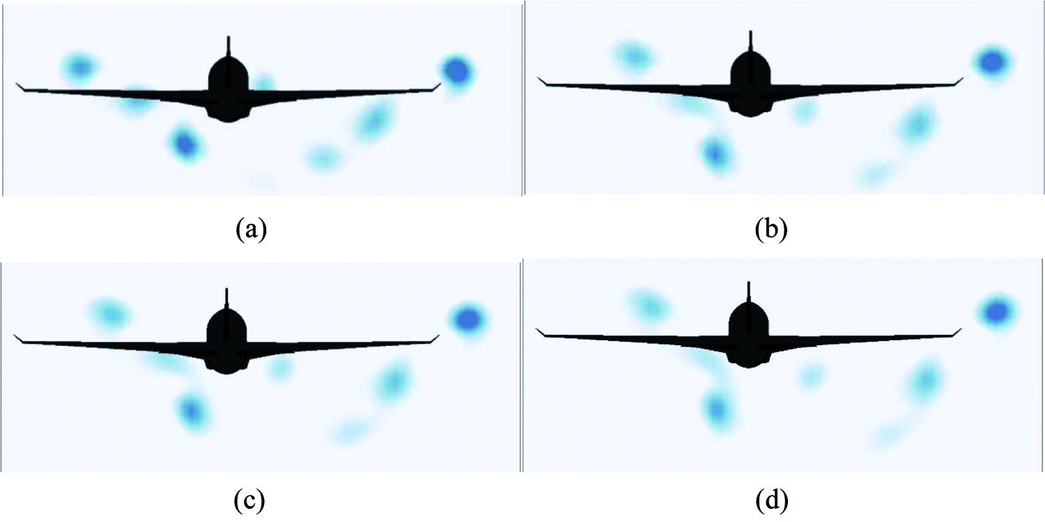
Figure 13: Contours at different positions under 5 m/s crosswind (Q criterion) (a) Twice the Wingspan (b) 2.5 Times the Wingspan (c) 3.0 Times the Wingspan (d) 3.5 Times the Wingspan

Horizontal motion is an important feature of wake vortices. These vortices can be blown out of the glideslope by accelerating their lateral motion in the approach phase. This can effectively reduce the safe approach separation between the preceding and following aircrafts, and improve the operation efficiency. Fig. 14 shows the variations of the four-vortex system in the YOZ plane under crosswind conditions. It can be noted that the wake vortices descend at a slower rate in the YOZ plane due to the energy input from crosswinds. It is found from comparison that due to effects from a left crosswind, the four-vortex system moves leeward as a whole and rotates and twists anticlockwise. As expected, a higher crosswind velocity causes the wingtip vortices to be blown faster out of the flight path. When the crosswind is equal to 5 m/s, the wake vortices at positions corresponding to a distance of 7.5 times the wingspan can be blown away from the runway for 20 m. Based on calculations for a runway width of 60 m in a single-runway airport, it can be gathered that wake vortices at positions greater than 1.4 km behind the fuselage can be completely blown away from the runway. Therefore, the effects on the following aircraft in the approach phase are small, and the takeoff separation can be significantly reduced compared with the current value of 5.6 km.

Figure 14: Vertex core distribution of four-vortex system in YOZ plane under different crosswind conditions (a) Movement trend of vortex system in YOZ plane under calm conditions (b) Movement trend of vortex system in YOZ plane under a 2 m/s crosswind (c) Movement trend of vortex system in YOZ plane under a 5 m/s crosswind

5  Conclusions

In this paper, numerical simulations of the A330-200 aircraft were carried out using the SST-RC model. The following conclusions are obtained based on the flow field analysis:

In the flow field of the whole aircraft, wake vortices had a complete four-vortex system structure, which was in two symmetrically distributed pairs. The two-vortex system at the outer side in the four-vortex system was formed due to the pressure difference between the upper and lower surfaces of the wingtip. The two-vortex system at the lower side was formed due to two reasons: 1) the pressure difference between the upper and lower surfaces of the wing root, 2) collision of the vortex resulting from the sweepback angle with the wingtip vortex of the horizontal tail when the former flowed through the horizontal tail.

The winglet could reduce wingtip vortices as it could split the wingtip vortices at the wingtip into two smaller streams of vortices. The streams initially developed separately and then merged into one vortex system at a position of 5 m behind the wingtip. The vortex system experienced energy dissipation during the merging process.

The dissipation of wake vortices was not perfectly positively correlated to crosswinds. Compared with the calm conditions, a 2 m/s crosswind could accelerate the dissipation of wake vortices at positions corresponding to a distance greater than 3.5 times the wingspan. Due to energy input from the crosswind in the case of a 5 m/s crosswind, both wingtip vortices downstream of the crosswind and wing root vortices upstream of the crosswind in the four-vortex system had a vorticity increase of about 68%. This created unfavorable conditions for reducing wake separation.

Crosswinds at a higher velocity could blow the aircraft wake vortices away from the flight path. Consequently, wake vortices at positions corresponding to a distance of 7.5 times the wingspan could be blown away from the runway centerline for 20 m, and the wake separation could be significantly reduced when only a runway width of 60 m was considered.

Acknowledgement: The authors would like to express their gratitude to Professor Weijun Pan of Civil Aviation Flight University of China for providing guidance and numerical simulation platform for this paper.

Funding Statement: This work was supported by the National Natural Science Foundation of China (Grant No. U1733203), and the Civil Aviation Administration of China’s Safety Capability Construction Program (Grant Nos. TM2018-9-1/3 and TM2019-16-1/3).

Conflicts of Interest: The authors declare that they have no conflicts of interest to report regarding the present study.

References

 1.  Hallock, J. N., Holzäpfel, F. (2018). A review of recent wake vortex research for increasing airport capacity. Progress in Aerospace Sciences, 98, 27–36. DOI 10.1016/j.paerosci.2018.03.003. [Google Scholar] [CrossRef]

 2.  Gerz, T., Holzäpfel, F., Darracq, D. (2002). Commercial aircraft wake vortices. Progress in Aerospace Sciences, 38(3), 181–208. DOI 10.1016/S0376-0421(02)00004-0. [Google Scholar] [CrossRef]

 3.  Hallock, J., Soares, M. (2007). Is the b757 really a “heavy” aircraft? 45th AIAA Aerospace Sciences Meeting and Exhibit. DOI 10.2514/6.2007-288. [Google Scholar] [CrossRef]

 4.  Liu, Z. R., Zhu, R. (2013). Dual wingtips vortexes Rayleigh-ludwieg instability experimrntal research. Journal of Experiments in Fluid Mechanics, 27(2), 24–30. DOI 10.3969/j.issn.1672-9897.2013.02.005. [Google Scholar] [CrossRef]

 5.  Gu, Y. S., Cheng, K. M., Zheng, X. J. (2008). Flow field characteristics of wing tips vortex and its control. Kongqi Donglixue Xuebao/Acta Aerodynamica Sinica, 26(4), 446–451. DOI 10.3969/j.issn.0258-1825.2008.04.006. [Google Scholar] [CrossRef]

 6.  Crow, S. C. (1969). Stability theory for a pair of trailing vortices. AIAA Journal, 8(12), 2172–2179. DOI 10.2514/3.6083. [Google Scholar] [CrossRef]

 7.  Corjon, A., Poinsot, T. (1996). Vortex model to define safe aircraft separation distances. Journal of Aircraft, 33(3), 547–553. DOI 10.2514/3.46979. [Google Scholar] [CrossRef]

 8.  Stephan, A., Holzäpfel, F., Misaka, T. (2013). Aircraft wake-vortex decay in ground proximity—Physical mechanisms and artificial enhancement. Journal of Aircraft, 50(4), 1250–1260. DOI 10.2514/1.C032179. [Google Scholar] [CrossRef]

 9.  Nybelen, L., Paoli, R. (2009). Direct and large-eddy simulations of merging in corotating vortex system. AIAA Journal, 47(1), 157–167. DOI 10.2514/1.38026. [Google Scholar] [CrossRef]

10. Misaka, T., Holzapfel, F., Gerz, T. (2013). Wake evolution of high-lift configuration from roll-up to vortex decay. 51st AIAA Aerospace Sciences Meeting Including the New Horizons Forum and Aerospace Exposition, pp. 1–11. Grapevine, Texas. [Google Scholar]

11. Holzäpfel, F., Stephan, A., Körner, S., Misaka, T. (2014). Wake vortex evolution during approach and landing with and without plate lines. 52nd Aerospace Sciences Meeting, Grapevine, Texas. [Google Scholar]

12. Holzäpfel, F., Stephan, A., Tchipev, N., Heel, T., Körner, S. et al. (2013). Impact of wind and obstacles on wake vortex evolution in ground proximity. Transactions of Japanese Society for Medical and Biological Engineering, 51, 2470. DOI 10.2514/6.2014-2407. [Google Scholar] [CrossRef]

13. Stuart, T. A., Mao, X., Gan, L. (2016). Transient growth associated with secondary vortices in ground/Vortex interactions. AIAA Journal, 54(6), 1901–1906. DOI 10.2514/1.J054484. [Google Scholar] [CrossRef]

14. Paramasivam, S., Skote, M., Zhao, D., Schlüter, J. U. (2016). Detailed study of effects of crosswind and turbulence intensity on aircraft wake-vortex in ground proximity. 34th AIAA Applied Aerodynamics Conference, Grapevine, Texas. [Google Scholar]

15. Misaka, T., Obayashi, S. (2017). Numerical study on jet-wake vortex interaction of aircraft configuration. Aerospace Science and Technology, 70, 615–625. DOI 10.1016/j.ast.2017.08.038. [Google Scholar] [CrossRef]

16. Lin, M. D., Cui, G. X., Zhang, Z. S., Xu, C. X., Huang, W. X. (2017). Large eddy simulation on the evolution and the fast-time prediction of aircraft wake vortices. Lixue Xuebao/Chinese Journal of Theoretical and Applied Mechanics, 49(6), 1185–1200. DOI 10.6052/0459-1879-17-198. [Google Scholar] [CrossRef]

17. Li, G. Z., Cao, Y. H. (2021). Numerical simulation of the wake generated by a helicopter rotor in icing conditions. Fluid Dynamics & Materials Processing, 17(2), 235–252. DOI 10.32604/fdmp.2021.014814. [Google Scholar] [CrossRef]

18. Ce, L., Pan, Y. C. (2020). Shear flows in the near-turbulent wake region of high speed trains. Fluid Dynamics & Materials Processing, 16(6), 1115–1128. DOI 10.32604/fdmp.2020.010829. [Google Scholar] [CrossRef]

19. Wu, W. M., Zhou, C. D. (2020). A numerical study of the tip wake of a wind turbine impeller using extended proper orthogonal decomposition. Fluid Dynamics & Materials Processing, 16(5), 883–901. DOI 10.32604/fdmp.2020.010407. [Google Scholar] [CrossRef]

20. Fourie, L. F., Square, L. (2020). Determination of a safe distance for atomic hydrogen depositions in hot-wire chemical vapour deposition by means of CFD heat transfer simulations. Fluid Dynamics & Materials Processing, 16(2), 225–235. DOI 10.32604/fdmp.2020.08771. [Google Scholar] [CrossRef]

21. Liang, Y. M., Yao, C. H., He, F. (2012). CFD-Based study of several geometrical parameters of winglet. Chinese Journal of Applied Mechanics, 29(5), 548–552+628. DOI 10.11776/cjam.29.05.A051. [Google Scholar] [CrossRef]

22. ANSYS Inc. (2010). ANSYS CFX-Solver theory guide. Pittsburgh: ANSYS Inc. [Google Scholar]

23. Qian, Y., Jiang, H. (2020). Numerical analysis of evolution process of vortex wake based on k-ω turbulent model. Science Technology and Engineering, 20(35), 14708–14713. DOI 10.3969/j.issn.1671-1815.2020.35.053. [Google Scholar] [CrossRef]

24. Yu, Y., Wei, Q. (1999). The structure of wingtip vortex and investigation for the model of wingtip vortex control. Acta Aerodynamica Sinica, 1999(4), 405–412. DOI 10.3969/j.issn.0258-1825.1999.04.007. [Google Scholar] [CrossRef]

This work is licensed under a Creative Commons Attribution 4.0 International License, which permits unrestricted use, distribution, and reproduction in any medium, provided the original work is properly cited.