Fluid Dynamics & Materials Processing

DOI: 10.32604/fdmp.2022.017737

ARTICLE

Application of the Navier-Stokes Equations to the Analysis of the Landslide Sediments Permeability and Related Seepage Effects

Meng Song1,*, Yuncai Liu2 and Zhen Wang1

1Huanghe Science and Technology College, Zhengzhou, 450063, China
2Gaoda Construction Engineering Co., Ltd. of Henan, Zhengzhou, 450063, China
*Corresponding Author: Meng Song. Email: wwz17z@163.com
Received: 02 June 2021; Accepted: 18 September 2021

1  Introduction

A landslide is a common geological disaster in many countries. It usually makes rocks or soil slide down from slopes, which is caused by gravity. Landslides often occur in mountain areas because tunnels are not constructed and the preventive measures are not carried out there. For example, when the water in the reservoir drops, the seepage of the slopes on both sides of the reservoir changes [1], and the permeability also changes, causing landslides. This demonstrates that the permeability of landslide sediments affects the structural stability of the reservoir. Therefore, it is valuable to study the characteristics of the seepage of landslide sediments and the hysteresis of water-borne landslide sediments, which has practical significance for the prevention and control of geological disasters in the area with a reservoir.

However, the research on the characteristics of the seepage of landslide sediments is complex because its characteristics are affected by many factors, such as the geology, the fluid, and the mechanical properties of rocks. Therefore, an experiment is carried out to simulate the research on the pressure of landslide sediment seepage with a computer. Fluid simulation is conducted with a computer, and Fluid-Structure/solid Interaction (FSI) simulation is most complex. The solid of the slope is affected by the vibration and deformation of fluids during landslides, and the flow velocity is changed, which is called fluid-solid coupling. However, most of the studies on fluid-solid coupling are focused on the boundary between the fluid and solid, and their simulation algorithms are too simple [2]. In fact, fluid-solid coupling happens between the sections of the solid and fluid and the influence of the properties between the two substances, which may change the physical properties of the two. In the previous studies, the flow velocity of fluids are calculated by Navier-Stokes equations [3].

Since the permeability has a great influence on the stability of slopes, the model of landslide sediments is implemented by using MATLAB to reconstruct its microstructure, and the change of the flow velocity of the landslide sediment seepage is simulated through built-in Navier-Stokes equations. After the change of the flow velocity caused by the concentration is analyzed, the post-processing software is used to process the calculated data so that the characteristics and influencing factors of the permeability of landslide sediments can be explored. Combined with the relationship between the cross-sectional velocity and the conditions of pressure, the seepage of landslide sediments is evaluated, and the rationality of the seepage law obtained by the simulation is verified.

Based on the previous studies and influencing factors of the permeability of landslide sediments, a microstructural model with pores of the landslide sediment is implemented by using three-dimensional modeling, the structure of the landslide sediment under pressure is analyzed, and the flow velocity is calculated according to the Navier-Stokes equation to study the characteristics of landslide sediments during seepage. After the simulation experiment, the fluid model implemented by the physical equation is discussed by analyzing its effectiveness and validity. The study provides a reference for the study of the pressure damage of landslide sediment seepage. The innovation of this study is to implement a model of the landslide sediment based on Navier Stokes equations to study the characteristics and mechanism of the permeability change of landslide sediments when the flow velocity changes.

2  Implementation of the Model of Landslide Sediments Based on Navier-Stokes Equations

2.1 Literature Review on Landslide Sediments

With rapid development of computer technology, there appear many new research means and methods to study landslide sediments. Zheng et al. [4] used different methods based on machine learning to identify potential landslides in the buffer zones of river basins. They also showed the morphology and texture characteristics of landslides according to the SAR deformation monitoring data, high resolution optical remote sensing data, and 17 influencing factors of landslides. They confirmed 83 areas, in which the landslide will happen, and 54 areas in which the landslide will not happen, and 64 areas in which there are potential landslides by analyzing the spatial superposition. Besides, they trained and tested Naive Bayes (NB), DT (Decision Tree), SVM (Support Vector Machine), and RF (Random Forest) algorithms through selecting attributes and optimizing parameters. Xiong et al. [5] studied the movement of landslides and their modes in valleys, as well as their gradient and particle size. They adopted PFC to carry out the experiment and implemented a numerical model of landslides. They found that the particles would collide with each other in the process of movement in the landslide; coarse particles were distributed on the front and surface of sediments, and fine particles were distributed on the back and bottom of sediments; the initiation angle has an influence on the morphology of the deposit. The larger the initiation angle is, the closer the deposit to the opposite bank of the valley is. Liu et al. [6] studied the feasibility when the reservoir water level before the flood season in the areas around the reservoir affected by the rainstorm. They calculated the rainfall of 20 counties from 1960 to 2010 according to Pearson and divided the annual rainfall data into four groups. Besides, they also estimated the parameters by fitting and verified them by the Kolmogorov-Smirnov test. Then, they proposed the reservoir decline model based on the actual reservoir regulation and analyzed the seepage of the Sifangbai landslide according to extreme rainfall and the reservoir decline model. The results show that the extreme rainfall in the flood season is 2.5, 1.4, and 2.2 times of the other three parts, respectively.

In short, the common methods used in the study of the existing landslide sediments are deep learning and a three-dimensional numerical simulation. Through the application of these new computer technologies, the hydrodynamic characteristics and the law of landslides are summarized, which is helpful to preventing and predicting landslides. The method used is the numerical simulation method.

2.2 Fluid Motion and the Navier-Stokes Equation

The determination of the fluid motion direction is mainly achieved by solving the Navier-Stokes equation to calculate the flow velocity. Since the fluid mechanism is introduced in the 18th century, its theoretical analysis and mathematical calculations are widely used to study the motion of fluids [7].

Navier-Stokes equations include mass conservation equations and momentum equations. According to the characteristics of different fluids, different hypotheses are made and different Navier-Stokes equations are obtained. The mass conservation equation shows the continuity of the fluid. In rectangular coordinates, the general form of the continuity equation of fluids is:

∂ρ∂t+∇⋅(ρu)=0 (1)

In Eq. (1), ρ is the density of the fluid, t is the time, u is the velocity vector, and ∇ is a divergent operator. u can be a two-dimensional vector or a three-dimensional vector according to the actual need.

For the fluid with a stable flow rate, the flow rate per unit time is regarded as a constant, which means that the density ρ is a constant, and the following equation is obtained:

∇⋅u=0 (2)

The differential expression derived from the momentum conservation law is:

∂u∂t=−(u⋅∇)u+f+∇⋅σρ (3)

f is the density function of the mass force, σ is the stress tensor, ∇ is the gradient operator, and the other parameters are the same as the above mentioned. If the fluid is incompressible (the divergence is 0), and it satisfies the condition of linear strain tension in the Newtonian fluid, the following expression is obtained when the viscosity coefficient is 0:

∂u∂t=−(u⋅∇)u+f−∇Pρ+v∇2u (4)

∇2 is the gradient divergence, and v=μ/ρ is the viscosity coefficient. The four expressions on the right side of the medium number are the horizontal transfer term, the external force term, the pressure gradient term, and the diffusion term, respectively.

The finite difference method is used in this study.

2.3 Construction of a Three-Dimensional Model of Landslide Sediments

The implementation of a three-dimensional model of landslide sediments is the first step to simulate the landslide sediment. And three-dimensional modeling methods mainly include the surface rendering method based on contour and the volume rendering method based on the equivalent surface [8]. The former can reflect the contour information of the model, but the information lacks internal details. The latter can calculate and extract the value of the internal structure of an object according to the collected data, and reflect its spatial structure. Three-dimensional objects contain both the surface contour structure and the internal structure. Three-dimensional modeling methods can represent geometric surfaces and usually take the voxel as the basic modeling unit. Therefore, the volume rendering method is suitable for voxel-based modeling. Compared with the surface rendering method, it can present more internal details. The specific steps are as follows: (1) assign different color parameters and transparency parameters to each data point; (2) integrate the pixels according to the corresponding lighting model to form the final image. Then, the data of landslide sediments obtained from the investigation [9] are calculated in the three-dimensional coordinate system. Thus, the gray information inside the structure is retained, which truly reflects the consistency between the virtual structure and reality. The model only considers the influence of single-phase water injection seepage, shortening the long simulation time [10].

Rock mass is composed of rock blocks with different shapes and structural planes. Therefore, the composition of sediments is very complex when landslides occur, which has a great influence on the study of physical and mechanical properties. When the crack size in the structural plane approaches a critical value, the structural parameters of the slope tend to be stable, which is called Representation Elementary Volume (REV). At present, most of the studies are mainly on the analysis of rock structure and mechanical properties to characterize the REV of rocks, and the studies on the the porosity is most. Porosity refers to the proportion of the pore volume to the total volume of porous materials, and it can reflect the structural characteristics of materials. Based on the REV, the structural characteristics of irregular shapes, like cylindrical and conical pores, are selected as the pore to simulate the model.

Joints, also known as fractures, are small fracture structures with no significant displacement on both sides of rock mass after its stress fracture, which have an important influence on the mechanical behavior of rock mass and cause the discontinuity, the heterogeneity, and the anisotropy of rock mass, as well as the change of rock mechanical parameters. Therefore, the equivalent calculation model of rock mass is implemented by combining the random joint three-dimensional network simulation technology with 3 Dimension Distinct Element Code (3DEC).

(1) First, a three-dimensional network model of random joints in the equivalent rock mass is implemented, and a block with a certain volume is established. The joint surface is determined according to the inclination of the joint, the point of the joint surface, and the penetration rate of the joint surface. Finally, the polygon joint surface is generated by cutting the block. The point passed by the joint surface is the coordinate of the center point of the disc joint. Joint surface penetration rate p can be calculated by Eq. (5):

p=aa+l (5)

In the equation, a is the diameter of the joint disc, l is the length of the intact rock in the extension direction of the joint surface. A three-dimensional network model of random joints in the equivalent rock mass is implemented by using the built-in FISH language according to the random number of joint inclination, dip angle, joint center point coordinates, and penetration rate.

(2) Second, the equivalent calculation model of rock mass is implemented. In the equivalent model, the rock block is processed by using the strain-softening model, which is based on the Mohr-Coulomb criterion. The shear failure is conducted according to the non-associated flow rule, and the tensile failure follows the associated flow rule. In the strain-softening model, two softening parameters need to be defined: shear softening parameter ks and tensile softening parameter kl. ks is the sum of plastic shear strain increment △ks, and kl is the sum of plastic tensile strain increment △kl. △ks and △kl can be calculated by Eqs. (6) and (7), respectively.

Δks=12(Δε1ps−Δεmps)2+(Δεmps)2+(Δε3ps−Δεmps)2 (6)

Δkl=|Δε3p1| (7)

In the above equations, Δε1ps and Δεmps are the plastic shear strain increments in the first and third principal stress directions.

Δεmps is the plastic shear strain increment for the body, and Δε3p1 is the plastic tensile strain increment in the direction of the third principal stress.

Δε1ps=λs (8)

Δε3ps=−λsNφ (9)

Δεmps=13(Δε1ps+Δε3ps) (10)

Δε3pl=λl (11)

s=fs(σ11,σ31)(α1−α2Nψ)−(α1Nψ+α2)Nφ (12)

Nψ=(1+sinψ)/(1−sinψ) (13)

Nφ=(1+sinφ)/(1−sinφ) (14)

In the above equations, ψandφ are the expansion angle and internal friction angle of rocks, respectively.

λl=(σ31−σl)/α1 (15)

α1andα2 are material constants defined by bulk modulus and shear modulus.

α1=K+4G3,α2=K−2G3 (16)

fs(σ11,σ31)=σ11−σ31Nφ+2CNφ (17)

σ11andσ31arethetrialstressintheiterativeprocess,andσl is the tensile strength of rock.

The failure of joints is divided into shear failure, tensile failure, compression-shear failure, and tensile-shear failure, which can be simulated by the Coulomb slip joint model. The calculation principle is as follows: the normal force loss Fn and tangential force vector Fis of joint surface contact are as follows in each calculation step:

Fn=Fn−knΔUnAc (18)

Fis=Fis−ksΔUisAc (19)

In the above equations, kn and ks are the normal stiffness and tangential stiffness of joint surface, ΔUn and ΔUis are the normal and tangential displacement increments of contact, and Ac is the contact surface area.

When the joint does not slip in the elastic range, the maximum tensile force and shear force of the joint surface are calculated by the following equations:

Tmax=−TAc (20)

Fmaxs=cAc+Fntanϕ (21)

In the above equations, T is the joint tensile strength, c and ϕ are the joint cohesion and internal friction angle.

When the joint is broken or sheared and the cohesion and tensile strength decreases to 0, the maximum tensile force of the joint is 0 and the maximum shear force is Fntanϕ . At the same time, the normal force and tangential force change accordingly: when the joint is a tensile fracture, the joint tangential force and normal force are released. When shear failure occurs, the normal force remains unchanged, and the tangential force is equal to the tangential force corresponding to the residual strength. The strain-softening is implemented on the rock, and the Coulomb slip mode is implemented on the joint, and the calculation grid is divided to implement the equivalent calculation model of rock mass.

Elastic deformation and plastic deformation have an important impact on the structural stability of the uniaxial compression simulation model. Because of this, it is necessary to select an appropriate elastic model and a plastic model. The plastic model usually constructs equations by Mohr Coulomb, which is simple and the parameter setting is clear:

F=c+σtan⁡φ (22)

F is the ultimate compressive stress, c is the cohesion in the structure and it varies according to the properties of the material, σ is stress, and φ is the friction angle. After the equation is selected, the LS-DYNA software is imported, and the simulation boundary conditions of the model are set based on the software. A uniform downward pressure load is set in the system to realize unidirectional compression. The simulation process is analyzed by the dynamic display, and the constraints are set under the model of landslide sediments to prevent the model from displacement in the simulation process.

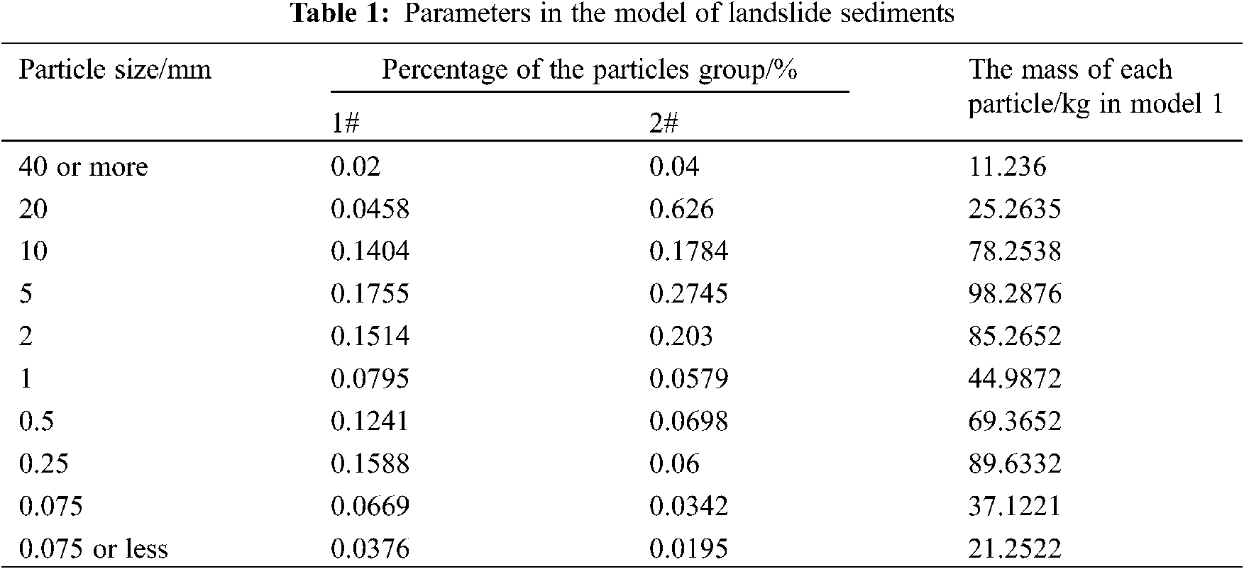
The parameters in the model of landslide sediments are shown in Table 1.

The different types of the models of seepage is shown in Fig. 1. The calculation of the model can be divided into 3 steps because the thickness and the slope of landslides are changed in the model. According to the survey, the seepage path of the landslide in Model 1 is set to be about 74 m, and the slope is set to be 24°. The seepage path of landslides in Model 2 is about 49 m, and the slope remains unchanged at 24°. The seepage path of the landslide in Model 3 is set to be about 74 m, and the slope is set to be 19°. The Geo-studio two-dimensional finite element numerical simulation software is used to implement the seepage/w module in the calculation model and encrypt the grid accuracy of landslides.

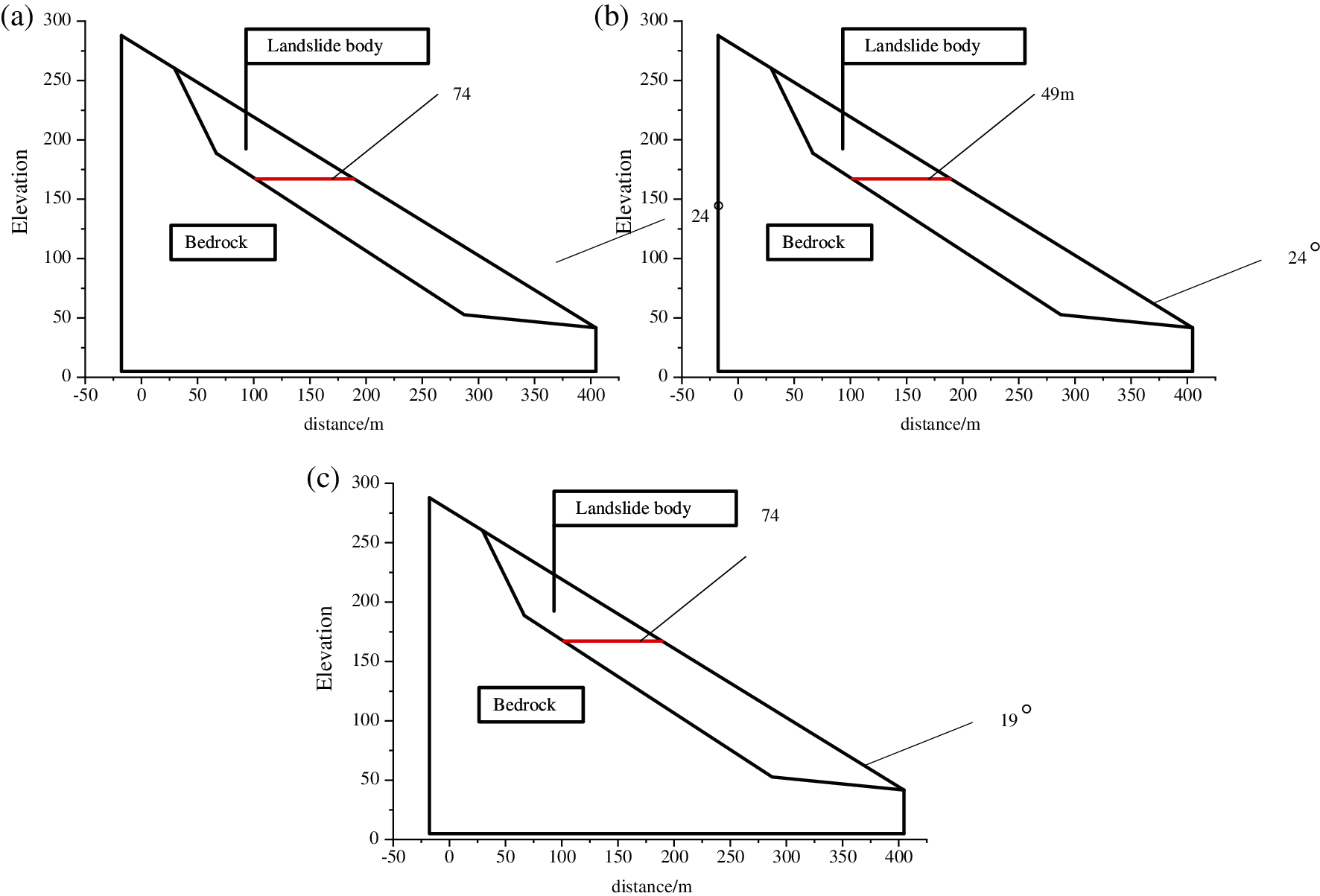
Figure 1: Calculation sections of different models (a) Calculation sections of Model 1; (b) Calculation sections of Model 2; (c) Calculation sections of Model 3

2.4 Construction of the Permeability Model of Landslide Sediments

It has great significance to improve the quality and efficiency of finite element analysis by using a powerful, convenient and flexible finite element pre-and post-processing tool that can be easily exchanged with many CAD systems and finite element solvers. HyperMesh is a popular pre-processing software at present. It has powerful and high-performance in finite element mesh pre-processing and post-processing. The three-dimensional solid model can also be directly imported into it. HyperMesh can provide a set of advanced, perfect, and easy-to-use toolkits for implementing the models, which greatly improves work efficiency. Here, HyperMesh software is used to simulate the construction of the model of landslide sediments, and then the data are imported into LS-DYNA software for calculation. The simulation mainly studies the permeability distribution and flow velocity changes of landslide sediments by calculating the flow velocity of the permeation, as well as the pressure. The model is set to have three elements: fluid, air, and the structure of landslide sediments. Among them, fluid provides kinetic energy and makes air enter the inner surface of landslide sediments.

Lagrange is selected as the main algorithm of the structure of landslide sediments, ALE is used to overcome the complex deformation of the grid caused by the fluid passing through landslide sediments, and the Navier-Stokes equation is used to calculate the flow velocity of fluids:

v∂vi∂t=∂ij,j+ρbi−ρwi∂vi∂xj (23)

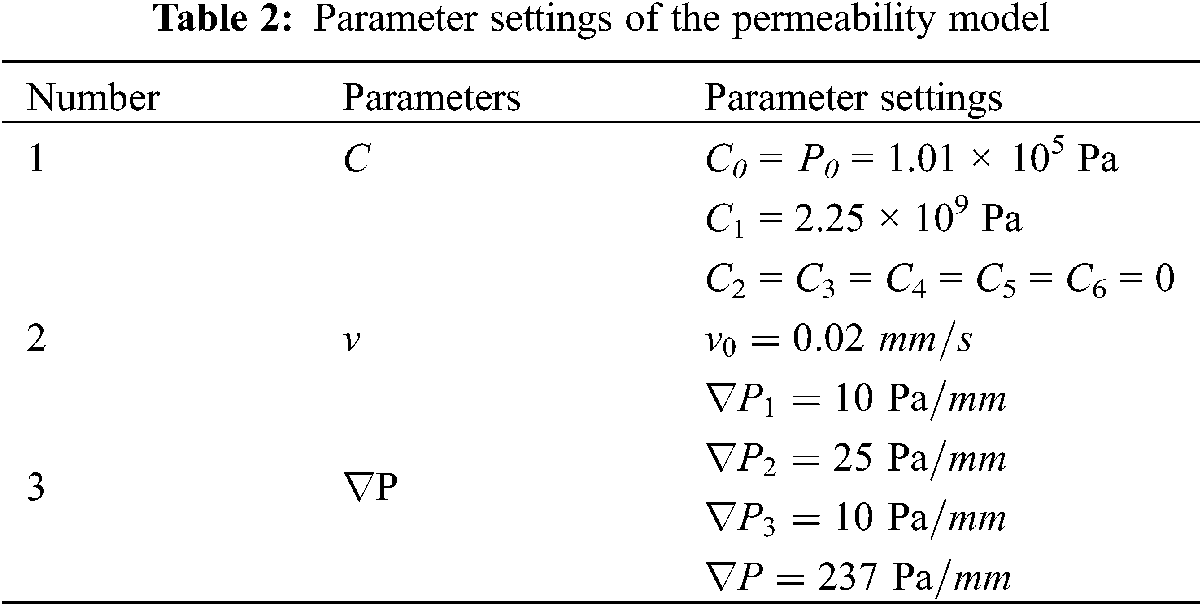
wi is the relative velocity of the fluid, and i and j are the coordinates in the rectangular coordinate system. The structure of fluids is analyzed by using the MAT-NULL model, which is suitable for exploring the properties of fluids. The air model is “MAT-VACUUM”. The linear polynomial equation can calculate the pressure change of fluids, which is expressed as follows:

P=(CO+C1μ1+C2μ12+C3μ13)+(C4+C5μ1+C6μ12)e (24)

Parameter C in the equation is the coefficient generated by the regional coordinate transformation.

P is the fluid pressure, e is the ratio of initial internal energy to fluid volume, μ=ρρo−ρl is the specific volume and C is the coefficient. The variables simulated by the model are shown in Table 2, and they are used to explore the influence of structural damage on permeability.

The fluid-solid coupling analysis needs to turn to ANSYS software. In the analysis process, the fluid and solid parts are separated. The first analysis is the load of the second analysis. If the analysis is completely coupled, the results of the second analysis will affect or become the load of the first analysis to couple the fluid and the solid. The analysis steps of fluid-solid coupling are as follows:

(1) Exporting solid CBD files and fluid CBD files in HyperMesh, and the fluid and solid grids are divided by HyperMesh.

(2) Importing the fluid grid.

(3) Setting analysis type, entering solid grid file, and setting transient analysis and time.

(4) Sorting fluid materials and setting properties.

(5) Setting the characteristics of the default domain in the flow field.

(6) Adding boundary conditions, which correspond to the boundary in the grid.

(7) Initialization.

(8) Solving control settings.

(9) Outputting control settings.

(10) Monitoring variable settings.

(11) Solving.

2.5 Algorithm Selection

The algorithm is the “operator” in numerical simulation and model simulation. The setting of the algorithm affects the accuracy and the calculation time of the simulation. The commonly used algorithms based on LS-DYNA software include the ALE algorithm, the Lagrange algorithm, and the Euler algorithm [11,12]. The Lagrange algorithm is used to deform the element mesh based on the material coordinates and the material flow. It can accurately describe the change of the structure of objects, but it is only applicable to the deformation of microstructure. The other two algorithms can overcome the computational problems caused by serious distortion. The Euler algorithm can realize material exchange and flow between nodes, but it is difficult to define the boundary motion suitable for analyzing the fluid motion. The ALE algorithm not only has the same accuracy as the Lagrange algorithm but also has the advantages of the Euler algorithm. Since the damage of fluids to the structure of landslide sediments is not discussed, the Lagrange algorithm is selected as the main algorithm in this study.

3  Analysis of the Simulation Results of the Permeability Characteristics of Landslide Sediments

According to the model of landslide sediments and the permeability model, the data during seepage are simulated by the software based on the relevant theory of the finite element, and the permeability distribution law and the stress mechanism of landslide sediments are explored.

3.1 Results of the Change of the Flow Velocity of Landslide Sediments

The increased process of fluids in landslide sediments is simulated, and the flow velocity is recorded when the landslide sediment is saturated. Table 3 shows the change of the flow velocity during the simulation experiment.

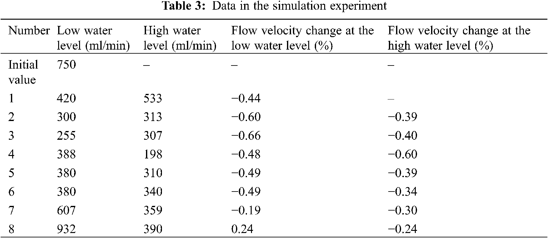
The table shows that the flow velocity at the low water level decreases by about 44% after the initial adjustment. And then the flow velocity continues to decrease after another two adjustments. It is relatively stable after the fourth to sixth adjustment and then continues to increase to 24%. However, the flow velocity at the high water level gradually decreases to 40%, and it begins to increase after the fifth adjustment but does not reach the initial value.

3.2 Changes of Surface Displacement

According to the simulation results of the model, the surface displacement and the deformation of the structure of landslide sediments are shown in Fig. 2.

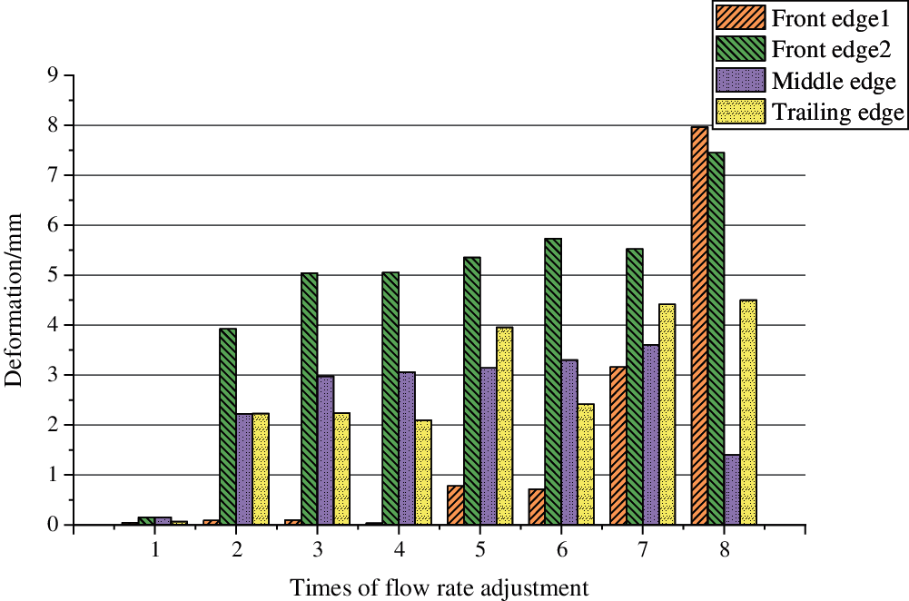
Figure 2: Deformation of the structure of landslide sediments

When the water level rises first, the structure of landslide sediments does not deform. However, the front part is gradually damaged, the surface becomes uneven, and the deformation of the middle and rear edges occurs as the flow velocity changes. The deformation of the front edge is large under the action of the water flow, and then the deformation becomes smaller and smaller gradually. Since the materials in the model are mainly soft rocks, the deformation speed and the degree of the slope are lower than hard rocks, and the deformation of the slope with little gravel is less than that of the slope with much gravel.

3.3 Permeability Characteristics of Landslide Sediments

At the initial velocity, the fluid enters the internal structure of landslide sediments from the pores. At this time, there is no obvious difference between pores during seepage. As time passes by, the pores are gradually connected. When the time of the flow reaches 40 s, the flow will reach the rear part of the landslide sediment. The cross-section analysis of landslide sediments shows that the flow velocity in the each section of pores will experience a dynamic process of “rising first and then falling”. VPeak and VStability represent the peak speed and the steady speed, respectively.

3.3.1 Influence of Different Deformation Degrees of the Model on the Permeability

The deformation degrees of the model of landslide sediments have a great influence on the permeability of water injection. According to the calculation of the overall axial stress of the model and the surface displacement, the pressure dropping along the tube is linearly fitted by using the incompressible viscous fluid when it flows steadily in the rough tube. The results are shown in Fig. 3. And the permeability of the structure of each model is evaluated [10].

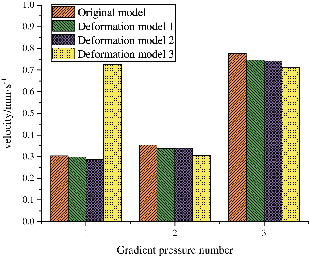
Figure 3: Permeability under different pressure

The figure shows that the permeability of the model is lower than that of the original model. With the increase of the displacement speed, the shape variable of the model is also increasing. This is consistent with the change law of the permeability of porous media geological materials during deformation [13]. The preliminary analysis shows that the reason for this result is that the main deformation of the model is elastic deformation, which reduces the pore composition of the model and leads to a decrease in permeability. However, as the deformation becomes inelastic, the internal structure of pores is torn and expanded, the porosity increases and the permeability increases accordingly. This shows that the permeability of landslide sediments is not only affected by the characteristics of its network structure but also closely related to the deformation of the structure.

3.3.2 Influence of the Deformation Degrees of the Structure of Local Pores on the Permeability

The axial stress εA, the radial stress εR, the peak velocity VPeak and the stable velocity stability of the measured structure of pores are statistically analyzed to clarify the reasons for the change of flow velocity in the pore. The changes of the three pores are shown in Figs. 4–6.

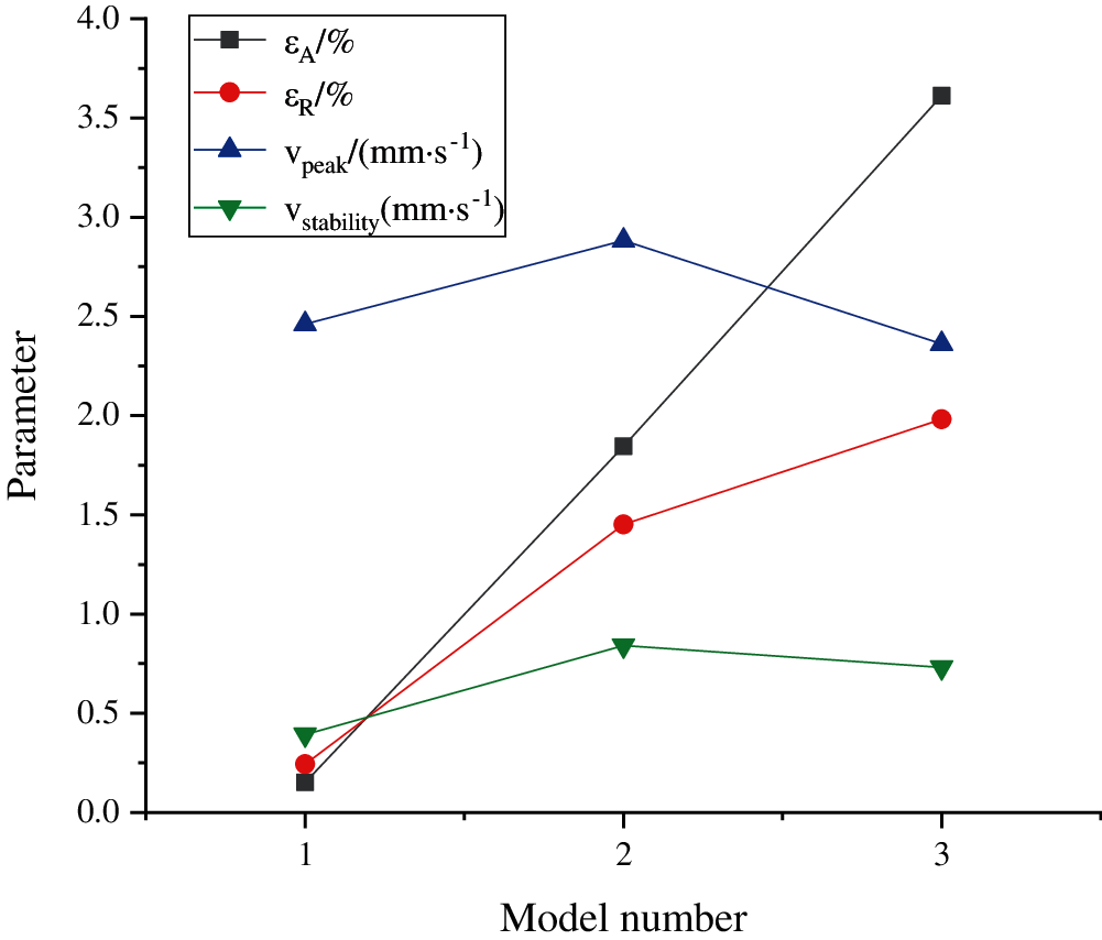
Figure 4: Changes of the structure parameters of No. 1 pore with the deformation of models

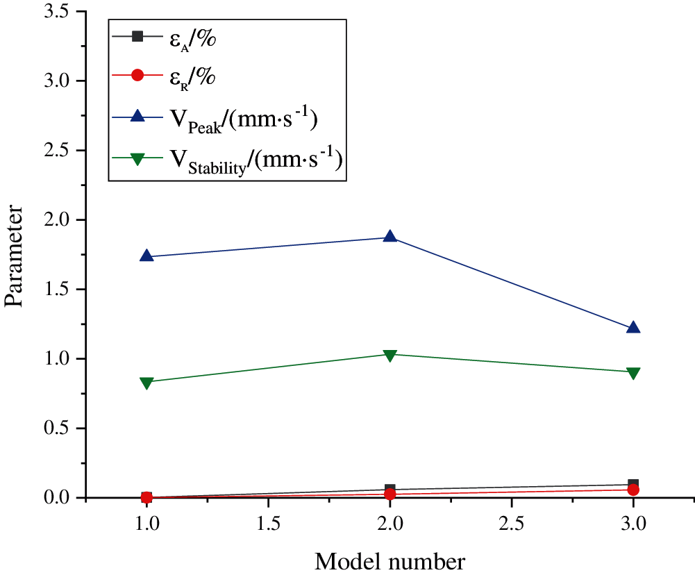
Figure 5: Changes of the structure parameters of No. 2 pore with the deformation of models

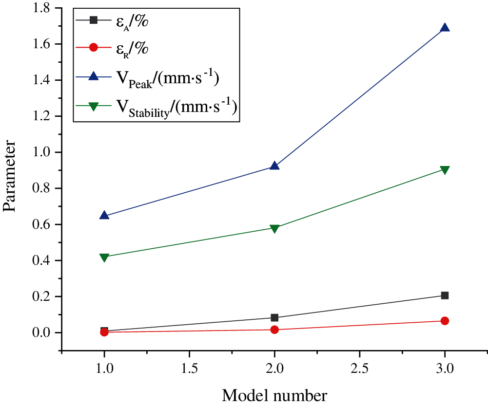
Figure 6: Changes of the parameters of No. 3 pore with the deformation of models

The figure shows that the values of the peak and the stable velocity increase first and then decrease with the increase of deformation degree in the structures of No. 1 and No. 2 pores. The gradual increase of deformation degree makes the peak and stable velocity values increase according to the stress distribution around the circular hole. In the structure of the No. 3 pore, the two parameters also gradually increase. According to the distribution and characteristics of the stress around the circular hole, the axial and radial stress affects the permeability of landslide sediments. In this case, the diameter of pores and the permeability decrease due to the axial deformation and increase due to the radial deformation. The results show that axial stress has a great influence on the change of the peak velocity in the structure of pores, and the stable change of the permeability is affected by the interaction of the axial stress and the radial stress. The deformation degree of the models does not change the flow velocity of pores. The increase of permeability in the front of the landslide sediment is affected by the overall deformation and leakage erosion, and the decline of the permeability in the middle and rear is due to landslides and collapses. After several tests on leakage, a more stable leakage passage of the slope is formed. Some pore leakage passages are compressed by the overall structure and continue to decrease. The other part of the pore structure is gradually penetrated by the fluid, and the leakage passage is continuously widened and the leakage ability is enhanced. And there are also some leakage passages and pore structures that decrease first and then increase. This shows that the structure of the model cannot change the trend of fluid leakage velocity in the pores over time, but it reduces the difference in the flow velocity.

3.4 Mechanism Analysis of Permeability Changes

According to the simulation experiment, the main influencing factors of the permeability of landslide sediments are the effect of seepage, the deformation of the internal structure, and the flow velocity. The effect of seepage on permeability is mainly manifested in latent erosion and blockage. Latent erosion is the particles of landslide sediments in the fluid, which increases the flow velocity caused by the increase of voids inside the landslide sediments. Usually, the front edge of landslide sediments is prone to subsurface erosion. Blockage refers to the deposition of fine particles in the structure of landslide sediments when landslide sediments are flowing with the fluid, which mainly occurs in the front edge of the landslide sediment, and the flow velocity is reduced.

According to the above data, it is found that the seepage flow of slopes changes with the change of water levels of fluids. Specifically, it decreases first and then increases, and the permeability changes similarly with the change of the seepage flow. If the seepage flow of landslide sediments is stable, the internal deformation makes the channel destroyed, and the local blockage of the landslide sediments makes the permeability of the whole slope decrease. The seepage channel will be re-formed in the slope after a seepage. In addition, the deformation and surface displacement occur in the interior of the slope, and the deformation cracks appear on the ground, which leads to the loose structure of landslide sediments and the low density and the enhanced permeability of the whole slope. This can be reflected by the increase of the seepage flow after the deformation of the slope. In terms of the influence of the water level on the permeability, the fluid force gradient in the slope is large and the permeability will increase when the water level increases, which accelerates the discharge of fine particles in the structure, resulting in seepage erosion.

The increase in the permeability of the front part of the landslide sediment is caused by the deformation and seepage erosion, while the decrease in the permeability of the middle and rear parts is due to the collapsibility of landslides. After the experiments, the slope is more stable. In the process of the simulation experiment, it is found that the change of the structure of pores is irregular, and the seepage channel of some pores receives the compression of the overall structure and decreases continuously; the other part of the structure of pores is gradually penetrated by the fluid, and the seepage channel in this part is continuously expanding and the seepage capacity is enhanced. However, some seepage channels decrease first and then increase. This indicates that the structure of the model cannot change the trend of the flow velocity of the fluid in the pore over time, but it reduces the difference in the flow velocity. Zhang et al. [14] described the effect of temperature on soil moisture when studying the phase change coupling algorithm of landslide sediments under the condition of ice-snow melting. The simplified algorithm is applied to the ice-snow melting coupling model of the landslide, and a practical numerical model is implemented for the coupling analysis of the temperature, the seepage, and the stress. A three-field coupled control differential equation is implemented to study the three-dimensional numerical simulation of stress, displacement, and plastic deformation. This study also uses the numerical simulation method to analyze and study the characteristics of landslide sediments, which provides support for the research in this field in future.

4  Conclusion

A simple structural model of landslide sediments is implemented based on the three-dimensional modeling technology to explore the influence of structural stress on the seepage of landslide sediments. On this basis, the simulation experiments of the stress and water injection during seepage are carried out. Through the analysis of the characteristics of the overall and local stress of different models, the following conclusions are drawn: (1) based on the basic principle of hydrodynamic equations, the fluid-solid coupling model is designed, and the Navier-Stokes equation is used to simulate the specific situation of fluids; (2) the results show that the internal deformation and expansion of landslide sediments are the main characteristics of the mechanical deformation of landslide sediments; (3) when the stress of internal structure of pores of landslide sediments increases, the shape of the internal structure of pores becomes the affecting factor of stress distribution. Through the analysis of various characteristics of the seepage and surface displacement of landslide sediments, it is found that the seepage of landslide sediments decreases first and then increases with the change of the water level of fluids, and the permeability also changes with the change of the permeability.

There are still some shortcomings of the study, which are summarized as follows: First, the design and solution of the Navier-Stokes equation should be more accurate, and more details should be satisfied to achieve a high-quality simulation effect; Second, only the influence of the porosity of the model during seepage is considered in the numerical simulation, which simplifies the design and shape of the structure of pores in the models, ignoring the influence of gravity. In the follow-up research, more accurate and reasonable algorithms should be introduced to optimize the research details of the characteristics of landslides during seepage, and the structure of pores in the model should be further studied to make the research results more universal and reliable.

Funding Statement: This work is supported by Science and Technology Public Project Fund of Henan Province (202102310567).

Conflicts of Interest: The authors declare that they have no conflicts of interest to report regarding the present study.

This work is licensed under a Creative Commons Attribution 4.0 International License, which permits unrestricted use, distribution, and reproduction in any medium, provided the original work is properly cited.