| Fluid Dynamics & Materials Processing |
DOI: 10.32604/fdmp.2022.018035
REVIEW
Review of Research Advances in CFD Techniques for the Simulation of Urban Wind Environments
1Tianjin Key Laboratory for Advanced Mechatronic System Design and Intelligent Control, School of Mechanical Engineering, Tianjin University of Technology, Tianjin, 300384, China
2National Demonstration Center for Experimental Mechanical and Electrical Engineering Education (Tianjin University of Technology), Tianjin, 300384, China
3School of Energy and Power Engineering, Shandong University, Jinan, 250061, China
4Shandong Engineering Laboratory for High-Efficiency Energy Conservation and Energy Storage Technology & Equipment, Shandong University, Jinan, 250061, China
*Corresponding Author: Pengfei Ju. Email: jupengfei_tjut@126.com
Received: 24 June 2021; Accepted: 22 September 2021
Abstract: Computational fluid dynamics (CFD) has become the main method for the prediction of the properties of the external wind environment in cities and other urban contexts. A review is presented of the existing literature in terms of boundary conditions, building models, computational domains, computational grids, and turbulence models. Some specific issues, such as the accuracy/computational cost ratio and the exploitation of existing empirical correlations, are also examined.
Keywords: Computational fluid dynamics; wind environment; pre-processing settings
With the acceleration of urbanization process worldwide, urban architecture with complex geometric structures and diverse layouts emerges in many countries, which has brought many wind environmental problems including but not limited to comfort, health, and energy efficiency, etc. For instance, the air velocity increases rapidly when the air flows between two buildings to an open area, which endangers the safety of pedestrians. This phenomenon is called the urban canyon effect [1]. Nature ventilation in urban buildings is suppressed due to the unreasonable structure and layout of nearby high-rise buildings, which leads to an increase of the building energy consumption [2–5]. The “vortex dead zone” phenomenon caused by unreasonable arrangement of buildings may severely obstruct the emission of harmful gases and waste heat, and also weakens the wind comfort at pedestrian height [6–9]. Therefore, the building wind environment prediction is of great significance for planning and shape designing of urban buildings [10].
At present, the main methods for studying the urban wind environment are field observation, wind tunnel test, and computational fluid dynamics (CFD) [11]. Observation helps obtain more accurate data for establishing a local wind environment database. However, the outdoor wind field is intrinsically unsteady and uncontrollable. It requires long observation period to obtain representative data. Therefore, the building surrounding flowfield observation is usually carried out after completion instead of the planning and design stage [12]. Field observation is now widely used for the validation of the CFD simulation and wind tunnel test.
The wind tunnel originates in the early 19th century. Early wind tunnel tests were mainly used to study the aerodynamic characteristics of aircraft rather than the urban wind environments. In the 1890s, Kernot et al. [13] used a wind tunnel to measure the surface wind pressure of a building model. Then in the 1930s, Bailey et al. [14] conducted a series of tests on the building model in an aviation wind tunnel and finally demonstrated the consistency of the model test data and building measured data under the shear flow condition. Jensen [15] further confirmed the feasibility of this method through the simulation of the atmospheric boundary layer in the wind tunnel according to the similarity criteria at the end of the 1950s.
There are many kinds of wind tunnels based on different functions. The so called “architectural wind tunnels” are specifically used to simulate the wind environment of buildings. The atmospheric boundary layer profile is firstly required and then reproduced in the wind tunnel in a specific test. The air flow generated by an upstream blower (or other similar devices) is sufficiently steady and controllable so that the flow field in the test section is in accord with the dynamic similarity law. The test model should also accord with the geometric similarity law. With the aid of several similarity criterion numbers, the test result of the test model can be easily converted into the “real” magnitude. Although the wind tunnel test provides a feasible approach to predict the huge flow field around urban building groups, there are still a lot of disadvantages. For instance, the wind tunnel test is difficult to meet the requirement of Reynolds number similarity [16], and geographical restrictions also make it unable to be carried out anytime and anywhere. The design and construction of a wind tunnel is very demanding in terms of money and time, so large scale wind tunnels are still valuable research facilities.
CFD emerged in the 1960s and has become the major method for the urban wind environment research after half a century’s rapid development [17]. Compared with wind tunnel tests, CFD is enable to build “actual-scale” simulation models [18]. There are no restrictions on boundary condition settings, which means that the target buildings can be studied under different weather conditions. Meanwhile, CFD can directly show the entire flow field in the computational domain and obtain the simulation results efficiently [19], while the wind tunnel test can only deliver data on a few selected points on and around the test model [20]. Errors also occur in CFD, such as the truncation errors caused by numerical schemes, model errors in turbulence models and boundary conditions, and the rounding errors caused by computer execution. All these errors influence the accuracy of the simulation results. Fortunately, many scholars have demonstrated great consistency of these two methods after a lot of comparations between CFD test results and wind tunnel test results [21–23]. CFD can effectively capture important physical phenomena, such as vortex shedding, air separation, and backflow, especially for single buildings.
CFD simulation can be divided into three steps: pre-processing, solver calculation, and data post-processing, among which the pre-processing is of most important for CFD operators because different preparations and settings will lead to significantly different results and unpredictable deviations. This paper summarizes the existing literature on CFD pre-processing from the perspective of the urban wind environment, especially on building external wind environment, in order to provide brief references for future researches.
Urban obstacles impose a relatively large drag force on the atmosphere. As the altitude increases, the wind speed increases until the wind speed is no longer affected by urban obstacles. This section of the atmosphere is called the atmospheric boundary layer (ABL) [24]. The height of ABL can change both in space and time, ranging from tens of meters to several kilometers depending on factors such as climate, landform, and season.
Fig. 1 depicts a cross section of a typical urban area, dividing the atmospheric boundary layer into two parts: the surface layer (SL) and the Ekman layer [25]. In the Ekman layer and free atmosphere, the Coriolis force, friction and pressure gradients influences the wind flow. Buildings are generally within the surface layer which is often considered to be neutral atmosphere. Therefore, the surface layer wind speed profile should be used as the inlet boundary condition of the computational domain in CFD. Two expressions can be used to describe the wind speed profile at the entrance of the computational domain with height, one is the exponential distribution and the other is the logarithmic distribution [21,26].
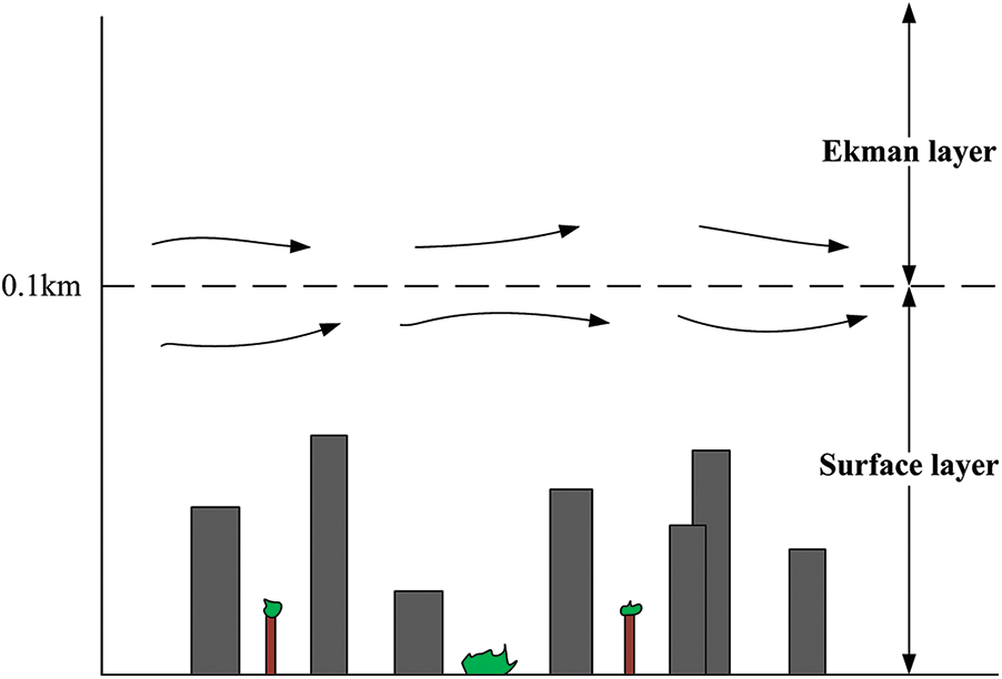
Figure 1: Schematic diagram of urban atmospheric boundary layer
2.1.1 Exponential Distribution
In 1916, G. Helleman proposed the exponential distribution law of the average wind speed in the atmospheric boundary layer. A. G. Davenport analyzed and summarized a large amount of measured data, which confirmed the scientific nature of G. Helleman’s viewpoint. A. G. Davenport also proposed a functional expression that satisfies the exponential distribution [27,28]:
In the above formula, z0 is the reference height (generally the height of the boundary layer). v0 is the wind speed at the reference height. z, vz are the desired height and the average wind speed at the desired height. α is a power index determined by surface roughness.
Many countries have corresponding guidelines for the value of α. For example, in Article 8.2 of China’s standard “GB50009-2012 Load Code for Building Structures” [29], the roughness of the ground is distinguished into four classes: maritime (A), rural (B), urban (C), and large-scale city (D). The value of α is taken as 0.12, 0.15, 0.22 and 0.30, respectively, and the height of the atmospheric boundary layer (gradient wind height) is respectively taken as 300, 350, 450 and 550 m. These values can generally meets the requirements of various projects. The roughness category of the selected area can be determined according to the average height of the building in the major wind direction within a radius of 2 km around the target building, which is expressed by h. If h ≥ 18 m, the roughness category will be D; if 9 m < h < 18 m, the roughness category will be C; if h ≤ 9 m, the roughness category will be B.
2.1.2 Logarithmic Distribution
For the stable surface layer, the wind speed profile can also be represented by a logarithmic distribution [30–32]:
In the above formula, z0, the height near the ground where the wind speed is 0, is the surface roughness length. v* is the friction speed, which usually does not change with height in the surface layer. z and vz are the required height and the average wind speed at the required height. κ is the von Karman constant, which is generally 0.4.
When simulating the wind environment of a building, the inlet boundary condition of the computational domain is generally velocity-inlet. The speed of the inlet is set by importing a user-defined function (UDF) into the commercial CFD software, and the speed direction generally selects the dominant wind direction in a certain period of time in the city.
2.2 Boundary Conditions for the Remaining Sections
When commercial CFD software is used to simulate the surrounding flow field outside, the airflow is generally not allowed to flow from the top or lateral boundary. “Symmetry” is usually prescribed as the boundary condition of these sections, which enforces a parallel flow, and the normal velocity component is zero. Therefore, the “blockage ratio” should be small enough to avoid artificial airflow acceleration. Sometimes, top and side boundaries of the computational domain are treated as “outflow” boundaries, which allows a normal velocity component outflow through the boundary. Therefore a smaller blockage ratio is also required to prevent the backflow in this case. At solid building walls and the ground, the “non-slip” condition is usually used.
Commercial CFD software usually delivers “outflow” or “constant static pressure” condition for the boundary behind the obstacles. The “outflow” boundary means that the derivatives of all flow variables are forced to vanish, corresponding to a fully developed flow. This boundary must be far enough from the obstacles to ensure the full development of the air flow and prevent any backflow.
3 Architectural Model and Computational Domain
A suitable architectural model and the appropriate size of the computational domain has a great impact on the accuracy and the time consumption of the simulation.
The architectural model contains not only the target building, but also the buildings, structures and terrain that have a great impact on it [33]. Therefore, it is important to identify whether the objects around the target building influence the wind field simulation. Referring to some wind tunnel tests, Frank et al. [34] concluded that for a building with a height of H, if the distance from the area of interest is larger than 6H, it can be ignored directly, and vice versa. This conclusion is regarded as the minimum requirements. It is better to perform testing simulations on the model with and without the building and make the decision after a case by case evaluation.
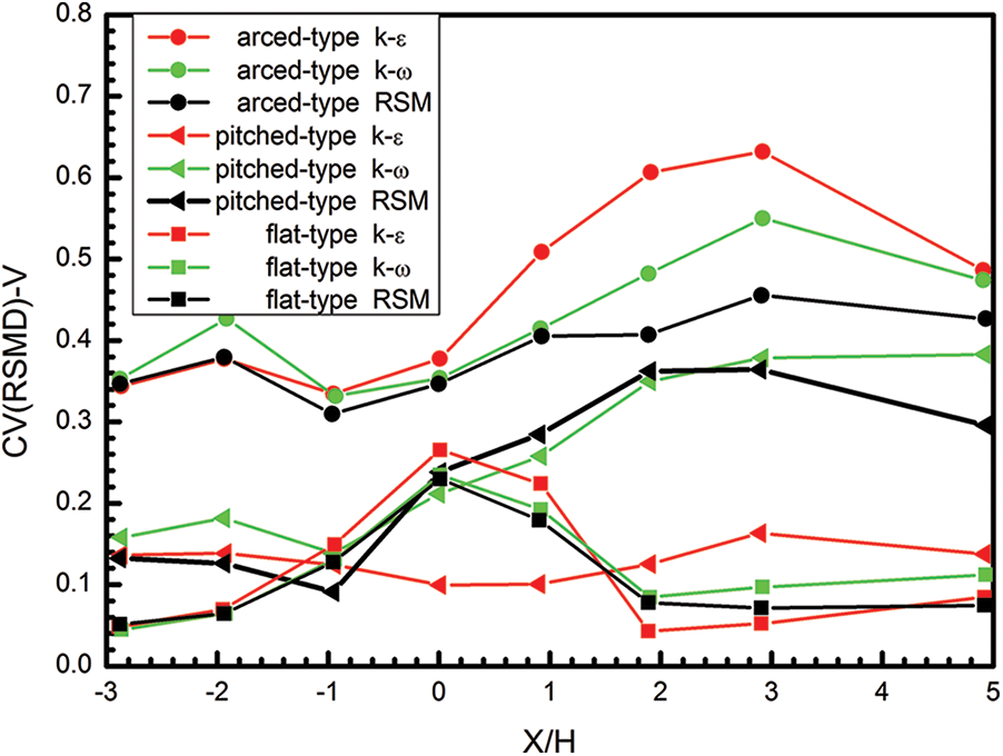
Figure 2: Simulation results of outdoor wind field of single building with different roof shapes (Data rearranged from literature [35])
Building shapes are becoming more and more diverse after years of development. Therefore, in order to make the simulation results more accurate, the actual building cannot be represented by either a square or rectangle in modeling [34]. The interested area should be modeled appropriately. Ntinas et al. [35] simulated a single building with different roof shapes (arced-type, pitched-type and flat-type roof) employing a variety of turbulence models, and found that the roof shape greatly affects the simulation results, as shown in Fig. 2. The ordinate (CV) in Fig. 2 means the mean square error of velocity.
Paying too much attention to the geometric structure of the model is not recommended. Excessively detailed geometric model will not only lead to the increase of the grid scale as well as cpu-time consumption waste, but also affect the accuracy of the calculation. Therefore, when simplifying the structure of a building model, it is better to examine the influence of the structure on the simulation results [36]. In order to shorten the verification process, the size of the computational domain including the target building should be reduced as much as possible. According to the comparison of the coarse mesh testing simulations, the final modeling is able to choose a reasonable geometric resolution [37]. Frank et al. [34] also summarized some empirical conclusions. For the building to be studied, the geometric structure larger than 1m should be described in detail. As for other buildings around the target building, the necessity of detailed structures depends on the distance. Buildings far away from the target building can be approximated by a square or rectangle.
The distances between the boundary of the computational domain and the area of interest in the vertical, lateral, and flow directions depend on the building model, which will affect the blockage ratio and the boundary conditions to be used. Frank et al. [34] proposed that the blockage ratio on these boundaries should preferably be less than 3%. The specific reasons have been explained in Section 1.2. For single buildings, the guidelines of Hall [38] can be used to determine the size of the computational domain. As shown in Fig. 3, the inlet, lateral and top boundaries should be 5H away from the target building, where H is the building height. However, in order to obtain a smaller blockage ratio, the distance on the outlet boundary should be at least 15H. For an urban area with many buildings, the above guidelines are still applicable, but the base height (H) consists with the height (Hmax) of the tallest building in the computational domain.
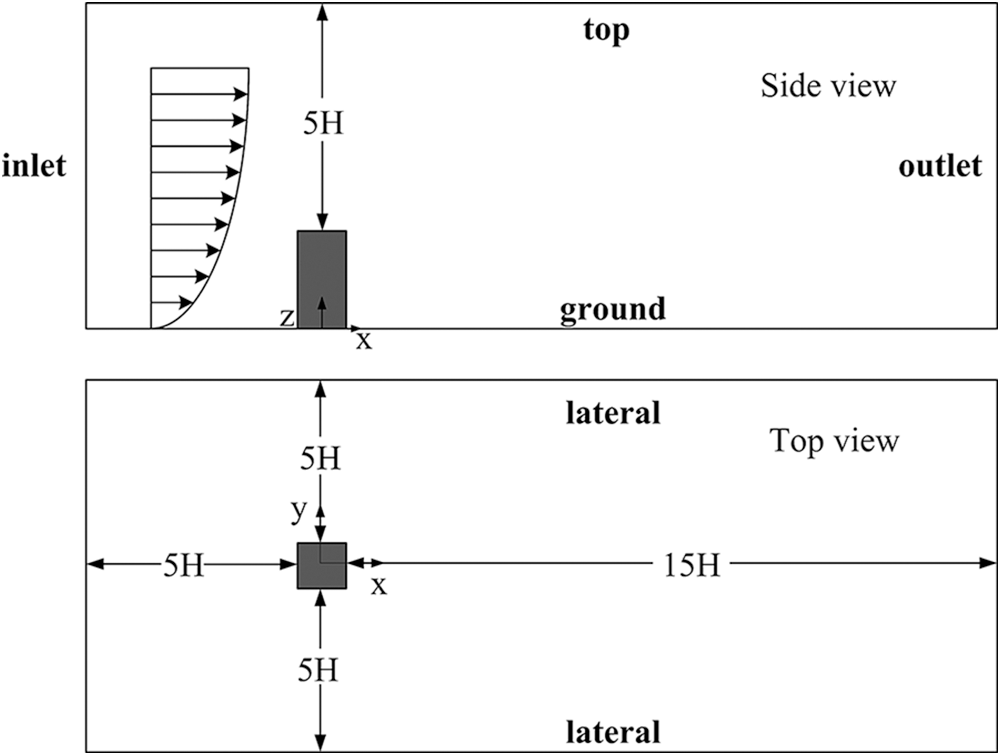
Figure 3: Computational domain determined by Hall: side view and top view
Although the guideline summarized by Frank et al. [34] is universal, the size of computational domain can be adjusted appropriately according to the required blockage ratio. For instance, Kaseb et al. [39] studied the influence of the building group layout on the wind speed at the pedestrian height. He took the distance between the outlet of the computational domain and the area of interest as 10 Hmax, and the distance between the inlet and the area of interest as 6 Hmax, and found that simulation results were not much different from the results of the wind tunnel test.
The resolution of the grid seriously affects the accuracy of the simulation results. Kim et al. [40] used grids with a size of 2.5 m × 2.5 m and 8 m × 8 m respectively to simulate a building area consisting of 9 high-rise buildings, and found that the velocity results between these two grids differs up to 11 m/s under certain wind direction.
Using grids with sufficiently high resolution can effectively capture some physical phenomena such as airflow separation and backflow on the building surface. However, if the grid in the computational domain is set too fine, it will increase the burden on the computer, and even reach an unbearable level [41]. Therefore, when simulating a single building, nonuniform grids of different resolutions are generally used. The finer grid should be used in regions of high gradients such as walls or ground [42], while the coarser grid locates far away from them. Fig. 4 shows an typical example consisting with the above viewpoints. Some scholars have obtained satisfactory simulation results on urban wind environment according to this principle [32,43,44]. For group buildings, the computational domain can be divided into three parts: the outside of the target area, the inside of the target area, and the vicinity of the wall. When generating the mesh, the mesh of the above three parts should be refined one by one [28,45]. Section 5 will describe the size of the first layer of grid on the wall.
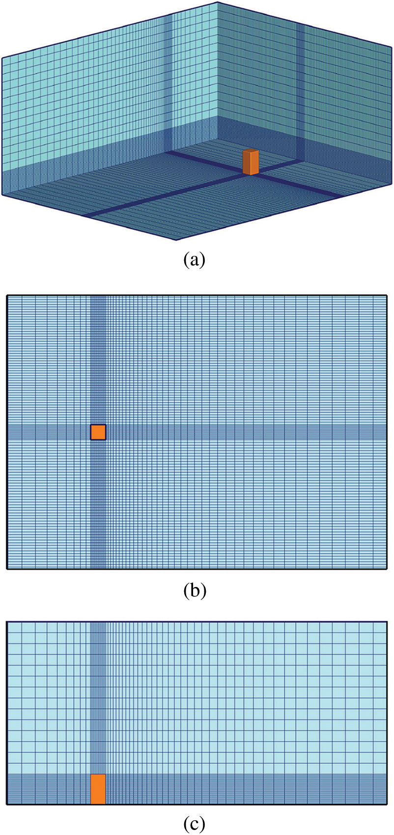
Figure 4: Hybrid mesh with different resolutions: (a) oblique view, (b) top view, and (c) front view
The quality of grid also greatly influences the simulation results. In the regions of high gradients, grid stretching or compression should be small enough to reduce the truncation error. Generally, the expansion ratio between two adjacent grids should be less than 1.3 in these regions [46]. The shape of the grid indirectly determines its quality. If the geometric structure of a single building or a group of buildings is relatively simple (usually represented by a cube), structural grids can be used near and away from the wall. Structured grids (generally regular quadrilaterals or regular hexahedrons) have better iterative convergence and smaller truncation errors, so its computational result is obviously better than that of the unstructured mesh. For buildings with complex shapes, a focus on structured grids can backfire, because the establishment of the structured grid requires a high degree of fitting between the block and the building model in order to achieve a better mapping effect. However, this is difficult for complex models. Therefore, it is recommended to use unstructured grids in areas of interest and structured grids far away from areas of interest for complex models. Some scholars used unstructured grids to simulate the wind environment outside the building, and it showed that the results were very satisfied [28,36,41,47,48]. Grid lines near the wall should be perpendicular to the wall. Therefore, if unstructured grids are used, prismatic girds should be used near the wall, and tetrahedral grids should be used far away from the wall [30,46].
Within a very small normal distance on the solid walls, the flow velocity will have a very large gradient. The flow velocity will decrease from a relatively large value to the velocity corresponding to the wall surface in the boundary layer. This area consists of three parts: viscous sublayer (linear sublayer), buffer layer, and logarithmic layer. Fig. 5 shows the relationship between u+ and y+ (see below) in the above three parts. The abscissa is the dimensionless distance normal to the solid walls (
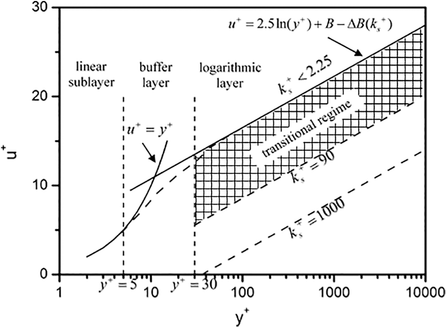
Figure 5: Dimensionless velocity distribution on smooth and rough surfaces
For the simulation of the flow field near the wall, two approaches are usually used: One is the wall function approach, and the other is the low-Reynolds number approach. The main difference between these two approaches is whether to resolve the viscous sublayer. Low-Reynolds number approach requires y+ < 1, where y+ means the thickness of the first layer of grid cells on the building wall. y+ < 1 ensures that the first layer of grid cells is in the viscous sub-layer, so the data of the viscous sub-layer can be obtained. This approach is generally used with low Reynolds number turbulence models (such as k-omega model, etc.) [46]. Wall function approach requires 30 < y+ < 500. In other words, using the wall function approach, the first layer of grid nodes apart from the wall should be in the logarithmic layer, so the viscous sublayer cannot be resolved. This approach is generally used with high-Reynolds number turbulence models (such as RNG k-ε model, Realizable k-ε model, and standard k-ε model, etc.) [46]. Therefore, the specific approach used depends on whether the CFD simulation needs to obtain the data of the viscous sub-layer. If necessary, the low-Reynolds number approach is used. If not required, the wall function approach is applicable.
In Fig. 5, the straight line with the characteristic of ΔB = 0 displays the dimensionless velocity distribution on smooth wall. For the rough wall, the slope of the dimensionless velocity distribution remains the same, but the intercept ΔB changes, which is a function of the roughness height ks+ (ΔB = 2.5ln(ks+)-3.3) [49]. According to the difference of ks+, the wall can be distinguished into three categories: aerodynamically smooth (ks+ < 2.25), transitional (2.25 ≤ ks+ < 90) and fully rough (ks+ ≥ 90).
The actual building surface and ground must be rough. When using commercial CFD software to simulate the flow field outside the building, the appropriate ks+ should be selected. For fully rough areas, ks+ ≈ 30z0 [46]. In this case, using the wall function approach, the resolution of the grid will be very low which is not conducive to capture the flow characteristics near the wall. However, if smaller ks+ is selected to enhance the grid resolution, the wind profile at inlet will change across the flow direction, which will affect the simulation results. Therefore, for the area with large roughness, if it is necessary to study the flow characteristics near the wall, it is better to use the low-Reynolds number approach by refining the grids on the wall. In the manuals of many commercial CFD software, the value ranges of y+ for different turbulence models have been indicated respectively, for the low-Reynolds number approach and the wall function approach.
At present, RANS is the most common way for simulating wind fields outside buildings. RANS involves various of turbulence models to express the so called “Raynolds Stress” item to close the time averaged Navier-Stokes equations. Considering different hypotheses for Reynolds stress modeling, RANS turbulence models are roughly distinguished into two types. The first type is based on the eddy viscosity hypothesis proposed by Boussinesq in 1877. This hypothesis believes that the Reynolds stresses are proportional to the mean velocity gradient, and the proportional coefficient is called the eddy viscosity. In order to solve the eddy viscosity, some variables are introduced. Turbulence models under this hypothesis can be further distinguished into zero-equation models, one-equation models (e.g., Spalart-Allmaras model) and two-equation models (k-ε model, k-ω model, etc.), according to the number of turbulence variables. The second type (Reynolds stress models, RSM; differential stress models, DSM) solves additional functions for derived Reynolds stresses [34]. A set of Reynolds stress transport equations not exceeding the second order have been established. However, the deteriorated computing stability and the more than doubled computing source occupying are still obvious disadvantages.
Large eddy simulation (LES) is a spatial filtering model between direct numerical simulation (DNS) and RANS. This model only distinguishes large scales of the flow and calculates them directly. Small scale eddies are spatially averaged and added to the entire flow field as additional model items.
When the wind flows around buildings, the streamline will be curved greatly. For example, there will be backflow at the downstream side of the building, and the top and corners of the building will contain flow separation [41]. Due to the introduction of the isotropic eddy viscosity hypothesis in the two-equation models, there is an error in simulating the roof of the buildings and the weak wind area behind them. Two-equation models often overestimate the reattachment length behind the buildings [34,35,43,46,50,51]. For instance, Shirzadi et al. [43] made a simulation of a building model using the standard k-ε model and compared with the experimental data, and confirmed the above statement. Fig. 6 shows a typical streamline diagram around a cube building near the ground. The simulation results of Ntinas et al. [35] shown in Fig. 2 also reflects the same conclusion.
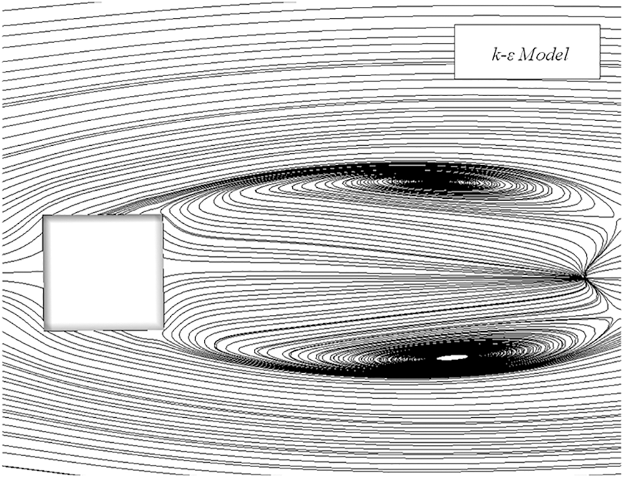
Figure 6: Streamline distribution of horizontal plane at 0.025 times of building height
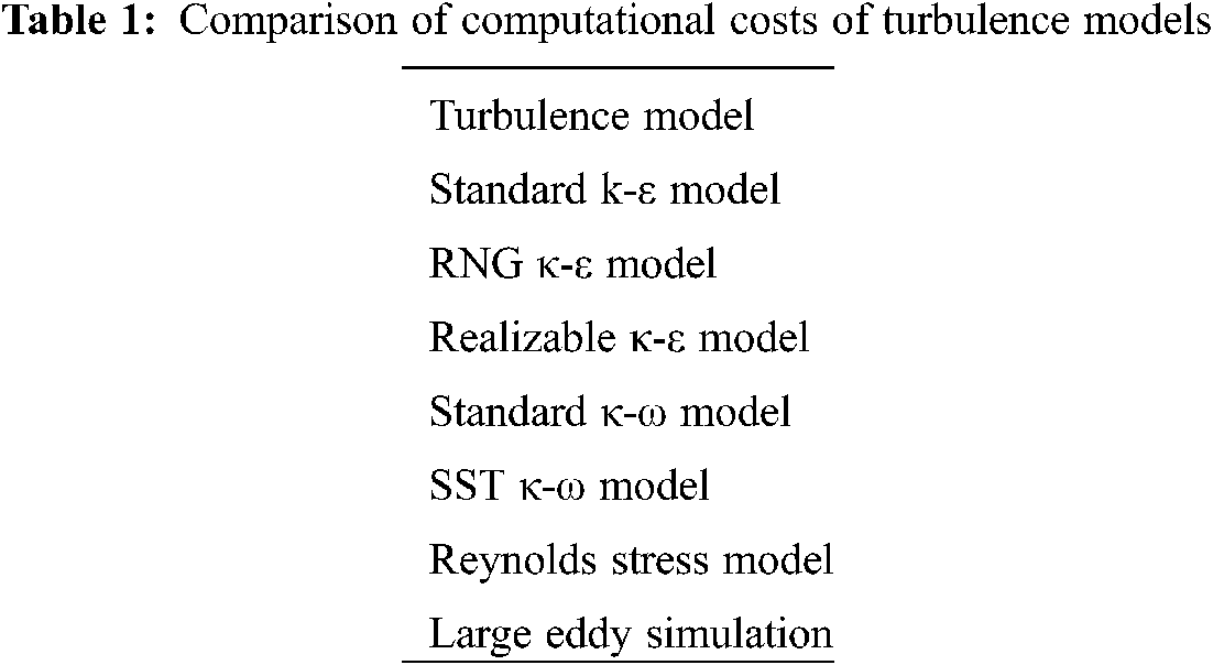
RSM and LES have got rid of the isotropic eddy viscosity assumption. Therefore, they can better reproduce main turbulence properties with a higher accuracy, compared with RANS [52–55]. But for now, the two-equation models are still much more popular. The main reason is that two-equation models cost much less CPU times compared with other models, and the calculation error level is still acceptable in engineering practices [34]. Table 1 lists a brief comparison of the calculational costs of the common two-equation models, RSM, and LES, increasing from top to bottom.
This paper respectively illustrates the influence of boundary conditions, architectural model, computational domain size, grid distribution and turbulence models on CFD simulation of urban wind environment. At the same time, it summarizes the experience and approaches of pre-processing proposed by some scholars. Here are the brief recommendations: (1) It is generally considered that most urban buildings are immersed in the neutral atmospheric boundary layer, and the average wind speed at the inlet boundary can be expressed as exponential distribution or logarithmic distribution along the height, while the flow direction is generally selected as the dominant wind direction in a certain period of time. (2) Lateral and top boundary of computational domain generally use “symmetry” or “outflow” conditions, both require a low blockage ratio. The purpose is to prevent artificial acceleration of the air flow for the “symmetry” condition, and to prevent air backflow for the “outflow” condition. The outlet boundary generally uses “outflow” or “constant static pressure” condition, and its location should be far enough away from the target area to approach the fully developed outflow and prevent backflow. (3) For a building with a height of H, it can be ignored directly as long as the distance from the interested area is greater than 6H. For the target object, the structures larger than 1 m are recommended to be modeled in detail, while objects far away from the target area can be approximated by a square or rectangle. (4) There are many empirical conclusions about the size of the computational domain. Guidelines for single building simulation are also useful for the building group case as long as the characteristic height is evaluated according to the tallest building. These restrictions in actual engineering practices can be relaxed according to the blockage ratio requirement. (5) Computational grids generally use nonuniform grids with different resolutions in different regions. Higher resolution is required in regions with high velocity gradient, and vise versa. The unstructured grid has an advantage in expressing complicated geometrical shapes, while prismatic grids are required near the wall or ground to ensure grid lines perpendicular to the boundary. (6) The wall function approach and the low Reynolds number turbulence model are two strategies for simulating flow in the wall boundary layer, and the two methods have different requirements for grid refinement near the wall. The former requires y+ < 1 for the first grid layer while the latter usually requires 30 < y+ < 500. (7) RANS simulations with the two-equation turbulence model are still the most popular strategy in this domain. However, certain errors exist because of the isotropic eddy viscosity hypothesis. RSM and LES can get rid of this theoretical defect, but their demand for computing resources is still beyond the current engineering practices can afford.
Funding Statement: This work was supported by the National Natural Science Foundation of China (No. 51976139).
Conflicts of Interest: The authors declare that they have no conflicts of interest to report regarding the present study.
1. Chang, C. H., Meroney, R. N. (2003). Concentration and flow distributions in urban street canyons: Wind tunnel and computational data. Journal of Wind Engineering and Industrial Aerodynamics, 91(9), 1141–1154. DOI 10.1016/S0167-6105(03)00056-4. [Google Scholar] [CrossRef]
2. Zhang, R., Mirzaei, P. A., Jones, B. (2018). Development of a dynamic external CFD and BES coupling framework for application of urban neighbourhoods energy modelling. Building and Environment, 146(3), 37–49. DOI 10.1016/j.buildenv.2018.09.006. [Google Scholar] [CrossRef]
3. Shirzadi, M., Naghashzadegan, M., Mirzaei, P. A. (2019). Developing a framework for improvement of building thermal performance modeling under urban microclimate interactions. Sustainable Cities and Society, 44, 27–39. DOI 10.1016/j.scs.2018.09.016. [Google Scholar] [CrossRef]
4. Allegrini, J., Dorer, V., Carmeliet, J. (2015). Coupled CFD, radiation and building energy model for studying heat fluxes in an urban environment with generic building configurations. Sustainable Cities and Society, 19(2), 385–394. DOI 10.1016/j.scs.2015.07.009. [Google Scholar] [CrossRef]
5. Norton, T., Grant, J., Fallon, R., Sun, D. W. (2010). Optimising the ventilation configuration of naturally ventilated livestock buildings for improved indoor environmental homogeneity. Building and Environment, 45(4), 983–995. DOI 10.1016/j.buildenv.2009.10.005. [Google Scholar] [CrossRef]
6. Moonen, P., Dorer, V., Carmeliet, J. (2011). Evaluation of the ventilation potential of courtyards and urban street canyons using RANS and LES. Journal of Wind Engineering and Industrial Aerodynamics, 99(4), 414–423. DOI 10.1016/j.jweia.2010.12.012. [Google Scholar] [CrossRef]
7. van Druenen, T.,van Hooff, T., Montazeri, H., Blocken, B. (2019). CFD evaluation of building geometry modifications to reduce pedestrian-level wind speed. Building and Environment, 163(11), 106293. DOI 10.1016/j.buildenv.2019.106293. [Google Scholar] [CrossRef]
8. Tsang, C. W., Kwok, K. C., Hitchcock, P. A. (2012). Wind tunnel study of pedestrian level wind environment around tall buildings: Effects of building dimensions, separation and podium. Building and Environment, 49(24), 167–181. DOI 10.1016/j.buildenv.2011.08.014. [Google Scholar] [CrossRef]
9. Tominaga, Y., Stathopoulos, T. (2011). CFD modeling of pollution dispersion in a street canyon: Comparison between LES and RANS. Journal of Wind Engineering and Industrial Aerodynamics, 99(4), 340–348. DOI 10.1016/j.jweia.2010.12.005. [Google Scholar] [CrossRef]
10. Wong, N. H., Jusuf, S. K., Tan, C. L. (2011). Integrated urban microclimate assessment method as a sustainable urban development and urban design tool. Landscape and Urban Planning, 100(4), 386–389. DOI 10.1016/j.landurbplan.2011.02.012. [Google Scholar] [CrossRef]
11. Ntinas, G. K., Shen, X., Wang, Y., Zhang, G. (2018). Evaluation of CFD turbulence models for simulating external airflow around varied building roof with wind tunnel experiment. Building Simulation, 11(1), 115–123. DOI 10.1007/s12273-017-0369-9. [Google Scholar] [CrossRef]
12. Blocken, B., Stathopoulos, T., Saathoff, P., Wang, X. (2008). Numerical evaluation of pollutant dispersion in the built environment: Comparisons between models and experiments. Journal of Wind Engineering and Industrial Aerodynamics, 96(10–11), 1817–1831. DOI 10.1016/j.jweia.2008.02.049. [Google Scholar] [CrossRef]
13. Kernot, W. C. (1893). Wind pressure. Journal of the Australian Association for the Advancement of Science, 5(H), 573–581. [Google Scholar]
14. Bailey, A. (1935). Wind pressures on buildings. Proceedings of the Institution of Civil Engineers-Civil Engineering. [Google Scholar]
15. Jensen, M. (1958). The model law for phenomena in the natural wind. Ingenioren International Edition, 2(4), 121–128. [Google Scholar]
16. Kubota, T., Miura, M., Tominaga, Y., Mochida, A. (2008). Wind tunnel tests on the relationship between building density and pedestrian-level wind velocity: Development of guidelines for realizing acceptable wind environment in residential neighborhoods. Building and Environment, 43(10), 1699–1708. DOI 10.1016/j.buildenv.2007.10.015. [Google Scholar] [CrossRef]
17. Blocken, B. (2014). 50 years of computational wind engineering: Past, present and future. Journal of Wind Engineering and Industrial Aerodynamics, 129(3), 69–102. DOI 10.1016/j.jweia.2014.03.008. [Google Scholar] [CrossRef]
18. Montazeri, H., Blocken, B. (2013). CFD simulation of wind-induced pressure coefficients on buildings with and without balconies: Validation and sensitivity analysis. Building and Environment, 60(2), 137–149. DOI 10.1016/j.buildenv.2012.11.012. [Google Scholar] [CrossRef]
19. Moonen, P., Defraeye, T., Dorer, V., Blocken, B., Carmeliet, J. (2012). Urban physics: Effect of the micro-climate on comfort, health and energy demand. Frontiers of Architectural Research, 1(3), 197–228. DOI 10.1016/j.foar.2012.05.002. [Google Scholar] [CrossRef]
20. Blocken, B., Stathopoulos, T., Carmeliet, J., Hensen, J. L. (2011). Application of computational fluid dynamics in building performance simulation for the outdoor environment: An overview. Journal of Building Performance Simulation, 4(2), 157–184. DOI 10.1080/19401493.2010.513740. [Google Scholar] [CrossRef]
21. Blocken, B., Stathopoulos, T. (2013). CFD simulation of pedestrian-level wind conditions around buildings: Past achievements and prospects. Journal of Wind Engineering and Industrial Aerodynamics, 121(10), 138–145. DOI 10.1016/j.jweia.2013.08.008. [Google Scholar] [CrossRef]
22. Lopes, M. F. P., Paixao Conde, J. M., Glória Gomes, M., Ferreira, J. G. (2010). Numerical calculation of the wind action on buildings using Eurocode 1 atmospheric boundary layer velocity profiles. Wind and Structures, 13(6), 487–498. DOI 10.12989/was.2010.13.6.487. [Google Scholar] [CrossRef]
23. Weerasuriya, A. U., Hu, Z. Z., Li, S. W., Tse, K. T. (2016). Wind direction field under the influence of topography, part I: A descriptive model. Wind and Structures, 22(4), 455–476. DOI 10.12989/was.2016.22.4.455. [Google Scholar] [CrossRef]
24. Bonner, C. S., Ashley, M. C. B., Cui, X., Feng, L., Gong, X. et al. (2010). Thickness of the atmospheric boundary layer above dome A, Antarctica, during 2009. Publications of the Astronomical Society of the Pacific, 122(895), 1122–1131. DOI 10.1086/656250. [Google Scholar] [CrossRef]
25. Britter, R. E., Hanna, S. R. (2003). Flow and dispersion in urban areas. Annual Review of Fluid Mechanics, 35(1), 469–496. DOI 10.1146/annurev.fluid.35.101101.161147. [Google Scholar] [CrossRef]
26. Xia, Q., Niu, J., Liu, X. (2014). Dispersion of air pollutants around buildings: A review of past studies and their methodologies. Indoor and Built Environment, 23(2), 201–224. DOI 10.1177/1420326X12464585. [Google Scholar] [CrossRef]
27. Sari, D. P., Gunawan, I., Chiou, Y. S. (2021). Investigation of Ecohouse through CFD Simulation. IOP Conference Series: Materials Science and Engineering.Vol. 1096, No. 1, pp. 12059. IOP Publishing. [Google Scholar]
28. Zhang, S., Kwok, K. C., Liu, H., Jiang, Y., Dong, K. et al. (2021). A CFD study of wind assessment in urban topology with complex wind flow. Sustainable Cities and Society, 71(5), 103006. DOI 10.1016/j.scs.2021.103006. [Google Scholar] [CrossRef]
29. MOHURD (Ministry of Housing and Urban-Rural Development of the People’s Republic of China) (2012). Load code for the design of building structures GB 50009-2012. [Google Scholar]
30. Prabhaharan, S. A., Rajasekarababu, K. B., Vinayagamurthy, G., Sivakumar, R. (2021). CFD simulation for pedestrian comfort and wind safety in VIT campus for wind resource management. IOP Conference Series: Materials Science and Engineering, vol. 1128, no. 1, pp. 12002. IOP Publishing. [Google Scholar]
31. Liu, S., Pan, W., Zhang, H., Cheng, X., Long, Z. et al. (2017). CFD simulations of wind distribution in an urban community with a full-scale geometrical model. Building and Environment, 117(4), 11–23. DOI 10.1016/j.buildenv.2017.02.021. [Google Scholar] [CrossRef]
32. Zheng, X., Montazeri, H., Blocken, B. (2020). CFD simulations of wind flow and mean surface pressure for buildings with balconies: Comparison of RANS and LES. Building and Environment, 173, 106747. DOI 10.1016/j.buildenv.2020.106747. [Google Scholar] [CrossRef]
33. Liu, S., Pan, W., Zhao, X., Zhang, H., Cheng, X. et al. (2018). Influence of surrounding buildings on wind flow around a building predicted by CFD simulations. Building and Environment, 140(4), 1–10. DOI 10.1016/j.buildenv.2018.05.011. [Google Scholar] [CrossRef]
34. Franke, J., Hirsch, C., Jensen, G. et al. (2004). Recommendations on the use of CFD in wind engineering. Proceedings of the International Conference on Urban Wind Engineering and Building Aerodynamics, pp. C.1.1–C1.11. COST Action C14. [Google Scholar]
35. Ntinas, G. K., Shen, X., Wang, Y., Zhang, G. (2018). Evaluation of CFD turbulence models for simulating external airflow around varied building roof with wind tunnel experiment. Building Simulation, 11(1), 115–123. DOI 10.1007/s12273-017-0369-9. [Google Scholar] [CrossRef]
36. Xu, F., Yang, J., Zhu, X. (2020). A comparative study on the difference of CFD simulations based on a simplified geometry and a more refined BIM based geometry. AIP Advances, 10(12), 125318. DOI 10.1063/5.0031907. [Google Scholar] [CrossRef]
37. Montazeri, H., Blocken, B., Janssen, W. D., van Hooff, T. (2013). CFD evaluation of new second-skin facade concept for wind comfort on building balconies: Case study for the Park Tower in Antwerp. Building and Environment, 68(2), 179–192. DOI 10.1016/j.buildenv.2013.07.004. [Google Scholar] [CrossRef]
38. Hall, R. C. (1997). Evaluation of modelling uncertainty. Study ling of near-field atmospheric dispersion. Project EMU final report. European Commission Directorate–General XII Science. Research and Development Contract EV5V-CT94-0531. Surrey: WS Atkins Consultants, Ltd. [Google Scholar]
39. Kaseb, Z., Hafezi, M., Tahbaz, M., Delfani, S. (2020). A framework for pedestrian-level wind conditions improvement in urban areas: CFD simulation and optimization. Building and Environment, 184, 107191. DOI 10.1016/j.buildenv.2020.107191. [Google Scholar] [CrossRef]
40. Kim, J. C., Lee, K. S. (2011). Effect of grid size on building wind according to a computation fluid dynamics simulation. Asia-Pacific Journal of Atmospheric Sciences, 47(2), 193–198. DOI 10.1007/s13143-011-0008-9. [Google Scholar] [CrossRef]
41. Mirzaei, P. A. (2021). CFD modeling of micro and urban climates: Problems to be solved in the new decade. Sustainable Cities and Society, 69(1967), 102839. [Google Scholar]
42. Liu, J., Niu, J. (2016). CFD simulation of the wind environment around an isolated high-rise building: An evaluation of SRANS, LES and DES models. Building and Environment, 96, 91–106. DOI 10.1016/j.buildenv.2015.11.007. [Google Scholar] [CrossRef]
43. Shirzadi, M., Mirzaei, P. A., Naghashzadegan, M. (2017). Improvement of k-epsilon turbulence model for CFD simulation of atmospheric boundary layer around a high-rise building using stochastic optimization and Monte Carlo Sampling technique. Journal of Wind Engineering and Industrial Aerodynamics, 171(A), 366–379. DOI 10.1016/j.jweia.2017.10.005. [Google Scholar] [CrossRef]
44. Tominaga, Y. (2015). Flow around a high-rise building using steady and unsteady RANS CFD: Effect of large-scale fluctuations on the velocity statistics. Journal of Wind Engineering and Industrial Aerodynamics, 142(2), 93–103. DOI 10.1016/j.jweia.2015.03.013. [Google Scholar] [CrossRef]
45. Jendzelovsky, N., Antal, R. (2021). CFD and experimental study of wind pressure distribution on the high-rise building in the shape of an equilateral acute triangle. Fluids, 6(2), 81. DOI 10.3390/fluids6020081. [Google Scholar] [CrossRef]
46. Franke, J., Hellsten, A., Schlünzen, K. H., Carissimo, B. (2007). Best practice guideline for the CFD simulation of flows in the urban environment-A summary. 11th Conference on Harmonisation within Atmospheric Dispersion Modelling for Regulatory Purposes. Cambridge, UK: Cambridge Environmental Research Consultants. [Google Scholar]
47. Shirzadi, M., Mirzaei, P. A., Tominaga, Y. (2020). CFD analysis of cross-ventilation flow in a group of generic buildings: Comparison between steady RANS, LES and wind tunnel experiments. Building Simulation, 13(6), 1353–1372. DOI 10.1007/s12273-020-0657-7. [Google Scholar] [CrossRef]
48. Kummitha, O. R., Kumar, R. V., Krishna, V. M. (2021). CFD analysis for airflow distribution of a conventional building plan for different wind directions. Journal of Computational Design and Engineering, 8(2), 559–569. DOI 10.1093/jcde/qwaa095. [Google Scholar] [CrossRef]
49. Hunt, J. C. R., Abell, C. J., Peterka, J. A., Woo, H. (1978). Kinematical studies of the flows around free or surface-mounted obstacles; applying topology to flow visualization. Journal of Fluid Mechanics, 86(1), 179–200. DOI 10.1017/S0022112078001068. [Google Scholar] [CrossRef]
50. Guo, H., Zhang, Z. (2021). CFD Analysis and optimization of an engine with a restrictor valve in the intake system. Fluid Dynamics & Materials Processing, 17(4), 745–757. DOI 10.32604/fdmp.2021.014651. [Google Scholar] [CrossRef]
51. Vardoulakis, S., Dimitrova, R., Richards, K., Hamlyn, D., Camilleri, G. et al. (2011). Numerical model inter-comparison for wind flow and turbulence around single-block buildings. Environmental Modeling & Assessment, 16(2), 169–181. DOI 10.1007/s10666-010-9236-0. [Google Scholar] [CrossRef]
52. Norton, T., Sun, D. W., Grant, J., Fallon, R., Dodd, V. (2007). Applications of computational fluid dynamics (CFD) in the modelling and design of ventilation systems in the agricultural industry: A review. Bioresource Technology, 98(12), 2386–2414. DOI 10.1016/j.biortech.2006.11.025. [Google Scholar] [CrossRef]
53. Hu, J., Huang, X., Jin, Y. (2021). A CFD study on a biomimetic flexible two-body system. Fluid Dynamics & Materials Processing, 17(3), 597–614. [Google Scholar]
54. Gousseau, P., Blocken, B., van Heijst, G. J. F. (2011). CFD simulation of pollutant dispersion around isolated buildings: On the role of convective and turbulent mass fluxes in the prediction accuracy. Journal of Hazardous Materials, 194(3), 422–434. DOI 10.1016/j.jhazmat.2011.08.008. [Google Scholar] [CrossRef]
55. Liu, C., Du, Y., Liang, J., Meng, H., Wang, J. et al. (2020). Large eddy simulation of gasoline-air mixture explosion in long duct with branch structure. Fluid Dynamics & Materials Processing, 16(3), 537–547. DOI 10.32604/fdmp.2020.09119. [Google Scholar] [CrossRef]
 | This work is licensed under a Creative Commons Attribution 4.0 International License, which permits unrestricted use, distribution, and reproduction in any medium, provided the original work is properly cited. |