| Fluid Dynamics & Materials Processing |
DOI: 10.32604/fdmp.2022.018434
ARTICLE
Optimization of the Structural Parameters of a Plastic Centrifugal Pump
School of Mechanical Engineering, Anhui Polytechnic University, Wuhu, 241000, China
*Corresponding Author: Yifang Shi. Email: 2200120112@stu.ahpu.edu.cn
Received: 24 July 2021; Accepted: 10 November 2021
Abstract: The structural design parameters of a plastic centrifugal pump were calculated and modeled, and flow field simulation analysis of the model was performed using CFD, in the framework of an orthogonal design method (or experiment). The inlet mounting angle β1, outlet mounting angle β2, wrap angle ϕ, and impeller inlet diameter D1 of the pump impeller were the four factors assumed for the application of the orthogonal experiment, using the efficiency and Net Positive Suction Head (NPSH) as evaluation indices. Moreover, taking the maximum efficiency and minimum NPSH of the plastic centrifugal pump as the evaluation factors, the parameters of the pump impeller were re-optimized through the Taguchi algorithm (leading to the following optimal combination: inlet diameter 35 mm, inlet angle 26°, outlet angle 27°, and wrap angle 110°). The minimum NPSH and the maximum efficiency have been found to be 0.957% and 61.5%, respectively.
Keywords: Plastic centrifugal pump; CFD; Taguchi algorithm
Plastic centrifugal pumps are widely used because of their strong suction capacity, low working noise, and leak-proof construction. However, the unreasonable structural design of some areas may bring serious harm to pumps’ operation, which hinders the development of plastic centrifugal pumps. At present, the research on the structure of plastic centrifugal pumps in the world is relatively mature. Plastic centrifugal pumps produced by large pump factories generally have the advantages of high rotational speed, small size, and light weight, but their performance indicators still need to be further improved, which requires further improvements to the pump mechanical structure [1]. In literature [2], the cavitation performance of a centrifugal pump with four different blade wrap angles was simulated. The influence of the four different blade wrap angles on the distribution of the bubble volume and pressure field of the centrifugal pump impeller was analyzed. However, the effects of other factors on the pump performance were not considered, and the data was not processed for further analysis. In literature [3], the cavitation characteristics of a centrifugal pump under small flow rates were studied. ANSYS CFX 14. 5 was used to numerically simulate the internal cavitation flow of an IS50-65-160 centrifugal pump with the impeller equipped with blades of 3 different numbers based on the k-ε turbulence model and Rayleigh-Plesset cavitation model. However, the number of subjects selected for this study and the number of simulation experiments were small; hence, the experimental results need further validation. In literature [4], the cause of “cavitation erosion” of cryogenic liquid pumps in air separation facilities and the characteristics of the pump itself were elucidated. Through analysis and testing, the design of the pump was improved to prevent “cavitation”, and then the anti-cavitation measures for cryogenic liquid pumps were proposed. However, these improvements were just proposed theoretically without experimental verification. In literature [5], numerical simulations were used to investigate the volute diaphragm mounting angle and its effects on the internal flow within a centrifugal pump. Based on the relationship between the specific speed and mounting angle of the volute diaphragm, four schemes of the volute diaphragm mounting angle were given, and Navier-Stokes equations and the SST (shear stress transmission) turbulence model were used to study the transient internal flow of the high specific speed centrifugal pump. In literature [6], with the main geometric parameters unchanged, a pump’s performance was optimized by reducing the effective flow area ratio of the inlet and outlet of the impeller flow channel with the help of the quasi-orthogonal method. Moreover, with an ultra-low specific speed centrifugal pump as the subject, based on the experimental results of the pump, seven impellers with different effective cross-sectional area ratios of the inlet and outlet of the impeller channel were constructed, and a complete geometric model including front and rear pump chambers and sealing rings was also constructed. With the help of CFD, the influence of different inlet and outlet area ratios on the performance and flow field structure distribution of the ultra-low specific speed centrifugal pump was analyzed. In literature [7], in order to study the influence of the blade wrap angle on the hydraulic characteristics of a double volute centrifugal pump, numerical simulations were used to study the external characteristics, internal flow field, the pulsation inside the volute at different wrap angles, followed by hydraulic performance experiments. In literature [8], a systematic study was conducted to analyze the method of meshing the computational domain, whether the flow state is steady or not, and the selection of turbulence models. Through theoretical analysis of the dynamic characteristics of the fluid particles in the impeller, the effects of the rotational centrifugal force, Coriolis force, and curved centrifugal force on the movement characteristics of the fluid particles in the impeller were identified, and ways for impeller hydraulic optimization were proposed. In literature [9], by combining the Powell vortex sound theory, numerical simulations and experimental measurements, this research explores the trends of variation and the corresponding underlying mechanisms for the flow-induced noise at various locations and under different operating conditions. It is shown that the total sound source intensity (TSSI) and total sound pressure level (TSPL) in the impeller, in the region between the inlet to the outlet and along the circumferential extension of the volute, are much higher than those at pump inlet and outlet. In literature [10], four geometrical parameters of the impeller are considered, i.e., the inlet diameter, the inlet width, the blade number, and the blade angle. The optimization is carried out on the basis of a three-level approach relying on an orthogonal test method. The results of the numerical simulations show good agreement with the experimental tests under different flow conditions. In accordance with the L9 (34) design table, the head and efficiency under the rated flow rate of the nine designed schemes are calculated and processed with the method of range analysis to obtain an optimized model.
In order to optimize the structure and performance of plastic centrifugal pumps, in this paper, CFD was used to analyze the flow field of a plastic centrifugal pump. Through the orthogonal experiment and range analysis, the combination parameters with efficiency and NPSH (net positive suction head) as evaluation indices were obtained. With the maximum efficiency and minimum NPSH as the evaluation indices of the combination parameters, the Taguchi algorithm was used to optimize the parameters of the analysis results; then, the optimal combination parameter with the maximum efficiency and minimum NPSH were obtained.
2 Structural Design of the Plastic Centrifugal Pump
The basic parameters of the plastic centrifugal pump are as follows: design flow rate Q = 4.5 m3/h, head H = 11 m, rotational speed n = 2840 r/min.
2.1 Design of the Plastic Centrifugal Pump Impeller
(1) The impeller’s inlet diameter D1 can be calculated from Eqs. (1) and (2):
where,
Q–flow rate (m3/s);
n–rotational speed (r/min);
k0–coefficient, which generally ranges from 3.5 to 4.0.
Considering cavitation and efficiency, k0 was taken as 4.5.
Then,
dh--the thickness of the shaft hole after opening the keyway (mm); take
Then,
(2) The impeller’s outlet diameter D2 can be calculated from Eqs. (3) and (4):
ns--specific speed; ns = 61.
Q--flow rate (m3/s);
n--speed (r/min).
Then,
(3) The impeller’s outlet width b2 can be calculated from Eqs. (5) and (6):
ns--specific speed;
Q--flow rate in (m3/s);
n–rotational speed (r/min).
Then,
(4) The impeller’s inlet width b1 can be calculated from Eqs. (7) and (8):
H--head (m);
K0--coefficient, which was set to 0.16.
Q--flow rate (m3/s);
ηv--volume efficiency, which was set to 0.973;
D1--blade’s inlet diameter (mm).
Then,
Then, the impeller inlet’s width b1 was taken as 5 mm.
(5) Mounting angle of blade’s inlet and outlet
It is recommended to set the blade’s inlet angle β1 to 20°∼25° and the attack angle Δβ = 3°∼15° for the highest hydraulic efficiency.
The blade’s inlet angle β1 was set to 10o∼40o. In order to gradually reduce the blade’s mounting angle on the streamline, β1 can be increased to optimize the shape of the impeller flow channel so that a balanced pressure of each impeller blade can be achieved for a favorable operating condition.
β1 = β1 + Δβ = 20°∼40°; set β1 = 25°. The blade’s outlet angle β2 is usually 16°−40°, but here β2 = 30°
(6) The number of blades Z can be calculated from Eq. (9):
D2--the impeller’s outlet diameter (mm);
D1--the impeller’s inlet diameter (mm);
β1, β2–the blade’s inlet and outlet angle.
Then, Z = 5.57; hence, the number of blades Z = 6.
(7) The thickness of blades s can be calculated from Eq. (10):
A--coefficient, related to the specific speed and material chosen; set A = 0.025;
D2--impeller’s outer diameter (mm);
Z--the number of blades;
H--the single stage head (m).
(8) The selection of the blade wrap angle
In general. The wrap angle can be taken as 90°∼120°. It should be taken slightly larger when the specific is relative low. Herein, the wrap angle was taken 110°.
2.2 Design of the Plastic Centrifugal Pump Volute
The base circle D3 tangential to the volute tongue should be slightly larger than the outer diameter D2 of the impeller to leave a proper gap between the tongue and the impeller. If the gap is too small, it may cause noise, vibration, and even cavitation in the tongue due to the blockage of liquid flow. Appropriately increasing the gap can lessen the flow blockage around the impeller, reduce noise and vibration, and improve efficiency. Herein, D3 was set to 131 mm; the volute’s inlet width b3 is usually larger than the impeller’s outlet width b2 so that the impeller’s front and rear covers can smoothly send the liquid into the pumping chamber and save part of the disk’s friction power to improve the pump’s efficiency. b3 was set to 10.9 mm; the mounting angle of the volute tongue Ψ0 should ensure the spiral session to be smoothly connected to the diffuser, and the radial dimension should be minimized as much as possible. Ψ0 was set to 15°.
The physical model of the impeller and volute flow channel was established based on the parameters above (see Fig. 1).

Figure 1: Fluid domain model
3 Numerical Simulation of the Internal Flow Field of the Plastic Centrifugal Pump
3.1 Boundary Condition Settings
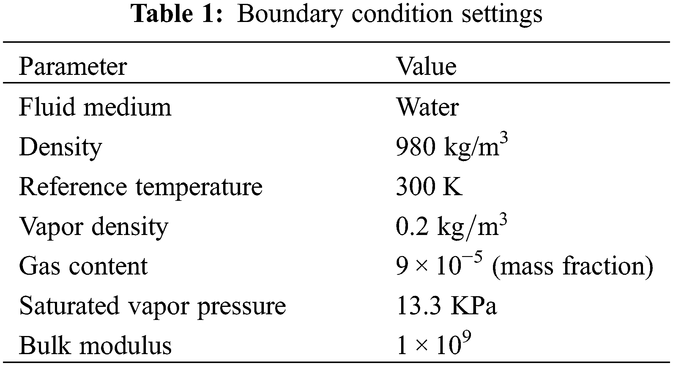
The boundary condition settings consist of the fluid medium’s basic properties [11], including its density, temperature, viscosity, gas content, steam density, saturated vapor pressure, etc., which are listed in Table 1. The boundary condition settings also relate to the rotor of impeller blades, the inlet and outlet of the fluid medium, and the rotating surface. Besides, the pump speed was set to 2840 r/min, the pump outlet flow rate to 0.00125 m³/s, and the inlet pressure to 1 standard atmospheric pressure.
The software defaults to the rotor being rotating and the volute and inlet being stationary. Therefore, the boundary condition settings should include the inlet, the rotor, and the interaction area between the rotor and the volute flow channel (see Fig. 2).

Figure 2: Interaction area
As only the k-ε model is suitable for processing the highly-bent streamline flow, it was selected as the calculation model for simulation. The continuity equation of incompressible fluid, the Reynolds time-averaged N-S equation and standard k-ε model were used to simulate the three-dimensional turbulent flow inside the impeller of the plastic centrifugal pump [12].
The standard k-ε model introduces the turbulent dissipation rate ε [13] based on the equation on the turbulent kinetic energy k, and its transport equation can be expressed as follows:
where,
Gk
Gb
μt
In Eqs. (13)–(15),
In the numerical calculation process, the fluid flow follows the law of conservation of mass, the law of conservation of momentum, and the law of conservation of energy. In this study, the medium of the model was water, which can be regarded as incompressible viscous fluid. The study was conducted at constant temperature, without considering the effect of temperature changes in the medium; hence the continuity equation and momentum equation is used to obtain solutions:
(1) continuity equation
where,
ρm—Density of the mixed phase (kg/m3);
ρk—Density of the k phase (kg/m3);
vm—Average mass;
vk—Relative velocity.
(2) Momentum equation
where,
F—Volumetric force (N);
μm—Viscosity coefficient of the mixed phase (Pa.s);
μk—Viscosity coefficient of the k phase (Pa.s);
αk—Volume fraction of the k phase;
vdr,k—Drift velocity of the k phase.
3.3 Meshing of Flow Part Model of the Plastic Centrifugal Pump
With the calculation accuracy and computer’s performance taken into consideration, the total number of mesh units was finally determined to be 181123. The results of mesh independence check are shown in Table 2.
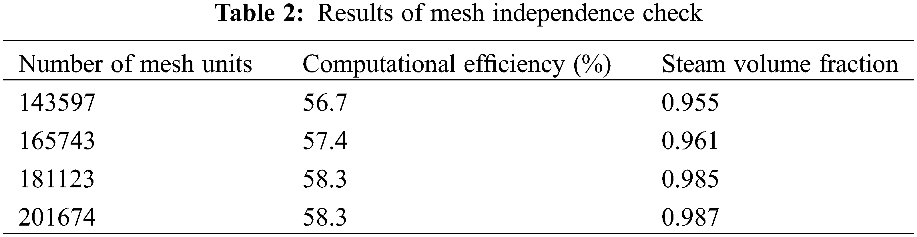
Meshing is the basis of numerical dispersion of flow control equations. The mesh quality directly affects the convergence and accuracy of results. As illustrated in Fig. 3, the mesh are unstructured, with 181123 mesh units. The mesh is three-dimensional, with the smallest unit being 0.0001 and the largest 0.025. After meshing, an entrance was added at the impeller’s inlet, and then the software could identify the entrance at runtime. The meshing after adding an entrance is shown in Fig. 4.

Figure 3: Meshing diagram

Figure 4: Meshing diagram after adding an entrance
3.4 Analysis of Simulation Results
The volute outlet pressure was monitored. When the outlet pressure was stable, it was considered as converged (see Fig. 5), according to which the outlet pressure value at this time was detected. According to the inlet pressure of the boundary conditions, the differential pressure of the plastic centrifugal pump at this operating point was obtained, and then the actual head and efficiency can be obtained.

Figure 5: Convergence graph
In the calculation, the SIMPLEC algorithm was used for the pressure-velocity coupling; the momentum equation, turbulent kinetic energy, and dissipative transport equation were in the second-order windward scheme. In the steady calculation, it converged when the total outlet pressure fluctuated steadily; the unsteady calculation converged when the monitoring results displayed a periodically stable distribution.
In the steady calculation, the “Frozen Rotor” model was used for the two interfaces between the inlet pipe and the impeller and between the impeller and the volute; the General Connection model was used for the interface between the volute and the outlet pipe for they were both stationary. In the unsteady calculation, the “Transient Rotor Stator” model was used for the two interfaces between the inlet pipe and the impeller and between the impeller and the volute, which can capture the interaction between the transient and the stationary state of the rotor in relative motion and take the steady calculation results as the initial conditions for the unsteady calculation [14].
The non-steady time step size Δt is defined as the impeller’s rotational angle at each computational step:
n--impeller’s rotational speed (r/min);
x--the rotational angle of the impeller in each time step.
With the computer memory and data integrity taken into consideration, x = 3°; that is, the impeller rotated once every 120 steps. The rated speed of the centrifugal pump n = 2840 r/min; then Δt = 0.0002 s. The convergence accuracy of the iterations in each calculational step was 1 × 10⁻⁵, and the maximum number of the iterations was 1000.
Convergence can be determined by monitoring the change in a physical quantity (such as pressure, power, etc.) at a specific position. When the physical quantity does not change as the iterations continue, or fluctuate slightly, convergence is reached. As the boundary conditions at the initial stage of the simulation were not unified, they were unstable. Therefore, the monitoring curve in the graph fluctuated in the beginning and stabilized later.
The fluid in the flow channel can only flow under pressure. As shown in Fig. 6, the blue area represents the highest pressure, and the red area the lowest pressure. The pressure was lowest at the inlet area, and the closer to the volute, the higher the pressure was. This pressure difference allowed the fluid medium to be sucked in and then transported.

Figure 6: Contour of pressure
The pressure increased gradually from the impeller’s inlet to its outlet without any noticeable sudden hike. The pressure was equally and reasonably distributed in each flow channel; hence, the design of the impeller was feasible.
Fig. 7 shows the flow velocity within the pump, wherein the fluid flow inside the impeller was even. The flow velocity near the outlet was significantly higher than that in other parts. The flow velocity was negatively related to the distance between the impeller and the pump shell wall. The overall distribution was reasonable.

Figure 7: Contour of velocity
3.5 Cavitation Simulation Analysis
Cavitation simulation involves multi-phase integrated simulation of a fluid medium. The bubbles are formed when the partial pressure is less than the vapor pressure of the medium. However, for different pumps and different media, the process is different. Herein, the Pumplinnx software was used to solve the momentum equation and volume ratio equation after the gas and liquid phases were mixed, and the cavitation was simulated.
As shown in Figs. 8 and 9, severe cavitation occurred at the impeller’s inlet and near the volute tongue, and its steam volume was as high as 0.99, which agrees with the actual situations. The pressure at the impeller’s inlet was so low that it reached the critical pressure of the medium vaporizing at room temperature, leading to severe vaporization. The flow condition near the tongue is complicated, which facilitates the backflow and vortex and affects the smooth flow of the medium. In addition to the rising pressure here, the steam bubbles began to burst, and the peak of the medium filled the cavity quickly, which stroke on the impeller and volute.
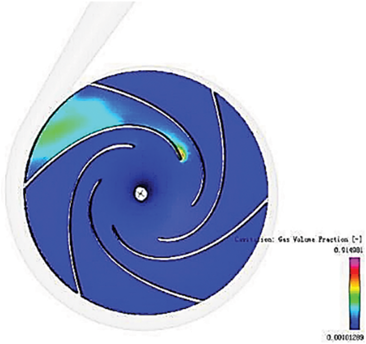
Figure 8: Vapor volume fraction

Figure 9: Vapor volume fraction
4 Orthogonal Experiment and Range Analysis of the Flow Field of the Plastic Centrifugal Pump
4.1 Orthogonal Experiment Design
The orthogonal experiment is a design scheme for multi-factor experiments by means of the normalized orthogonal tables in mathematical statistics. The basic steps are as follows:
(1) Selecting experimental objectives and indices
When the selected parameters were applied to the orthogonal experiment, the experimental indices and quality evaluation indices were decided.
(2) Selecting experimental factors and their levels
In the experiment, the factors were represented by English alphabets such as A, B, C. In selecting the factors, the factors that had more significant impacts on the experiment evaluation indices were prioritized. Then, the level of each factor was determined based on relevant information. In order to ensure experimental efficiency, 2 to 4 factor level values were chosen. The spacing of the factor level values was determined based on the existing reference data and professional information with the best effort to make the values at each level within the appropriate range.
Several factors may affect the efficiency and vapor volume fraction in the experiment. It is not feasible to include all of them into the orthogonal experiment. According to the relative theories and practices, the impeller’s inlet angles, outlet angles, wrap angles, and inlet diameters were selected as the four major factors. The selected factors and levels are listed in Table 3. For convenience, the letters A, B, C, and D represent the inlet diameter D1, inlet angle β1, outlet angle β2, and warp angle, respectively.
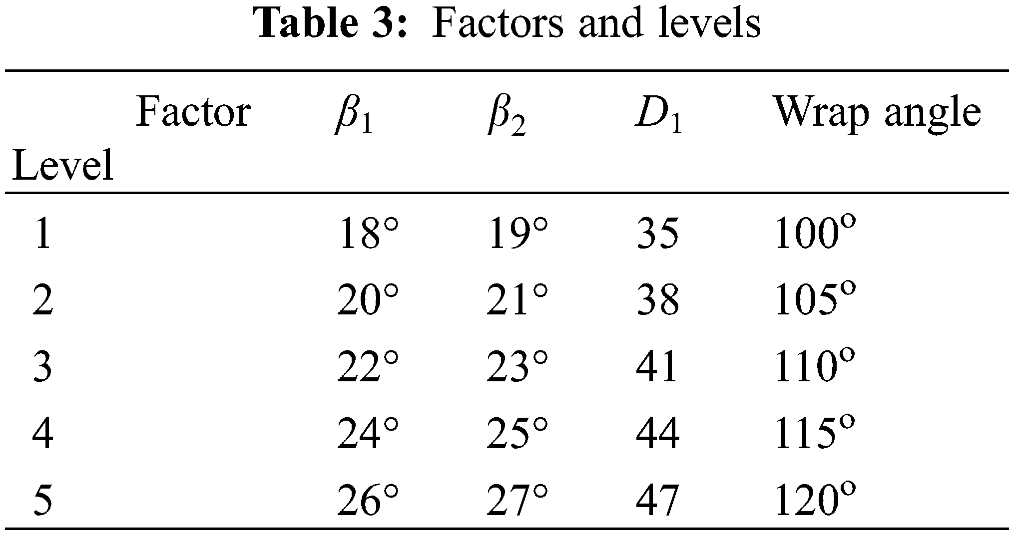
The orthogonal table of four factors and five levels was L25 (54). Orthogonal experiment results of the plastic centrifugal pump are presented in Table 3.
4.3 Experimental Index Determination
In this experiment, the efficiency and vapor volume fraction were the indices.
4.5 Data Processing of Experimental Results
By calculating the R-value of each parameter according to the experimental results in Table 4, the influence of each factor (index) is presented in Tables 4 and 5.
(1) With cavitation, that is, vapor volume fraction as the evaluation index, results are displayed in Table 5.
(2) With efficiency as the evaluation index, results are shown in Table 5.
4.6 Analysis of Experiment Results
(1) Analysis of vapor volume fraction
As per Table 5, K1, K2, K3, K4, K5 refer to the sum of vapor volume fraction of each factor under the levels of 1, 2, 3, 4, and 5, respectively, while k1, k2, k3, k4, and k5 represent the average value of vapor volume fraction of each factor. The range value R reflects the influence of each factor. According to the evaluation index, the optimal combination was A2B5C5D3, wherein the outlet diameter was 38 mm, inlet angle 26°, outlet angle 27°, and wrap angle 110°, and the vapor volume fraction reached its minimum. The optimized process parameters were not available in the existing experiment. The steam mass fraction of this set of data was 0.957, which was verified using Pumplinx simulation software. Comparing the size and location of the vapor volume fraction with the existing 25 sets of experimental results, the vapor volume fraction was close to the minimum value in the experiment, and the cavitation was significantly improved. The experimental results are presented in Figs. 14–17.

Figure 14: Line chart of the influence of each factor on vapor volume fraction
Figure 15: Vapor volume fraction (minimum NPSH)

Figure 16: Contour of velocity (minimum NPSH)
Figure 17: Contour of pressure (minimum NPSH)
By analyzing the results of the orthogonal experiment with the range method, the influence of each factor on each evaluation index was obtained: inlet angle > wrap angle > inlet angle > inlet diameter.
(2) Analysis of efficiency
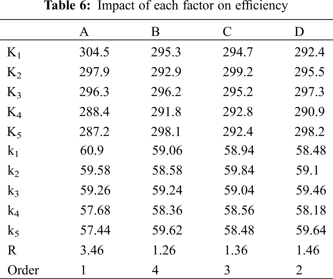
As per Table 6, K1, K2, K3, K4, K5 respectively stand for the sum of the efficiency of each factor under the levels of 1, 2, 3, 4, and 5, while k1, k2, k3, k4, and k5 represent the average value of efficiency of each factor. The range value R reflects the vapor volume effects of each factor. According to the evaluation index, the optimal combination was A2B5C5D3, wherein the outlet diameter was 35 mm, inlet angle 26°, outlet angle 21°, and wrap angle 120°; also, the vapor volume fraction reached its maximum. The optimized process parameters were not existing in the existing experiment. The efficiency of the data was 61.4% using Pumplinx simulation software. By comparing the existing 25 groups of experiment results, it can be found that the efficiency was close to the maximum in the experiment. The experimental results are shown in Figs. 10–13, 18–21.

Figure 10: Vapor volume fraction (experiment 1)

Figure 11: Vapor volume fraction (experiment 7)

Figure 12: Vapor volume fraction (experiment 15)
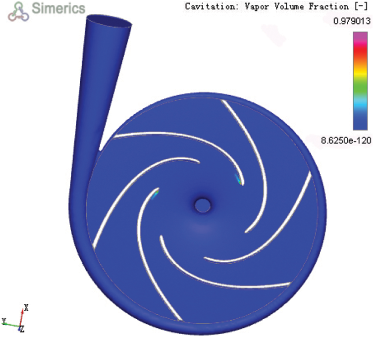
Figure 13: Vapor volume fraction (experiment 23)
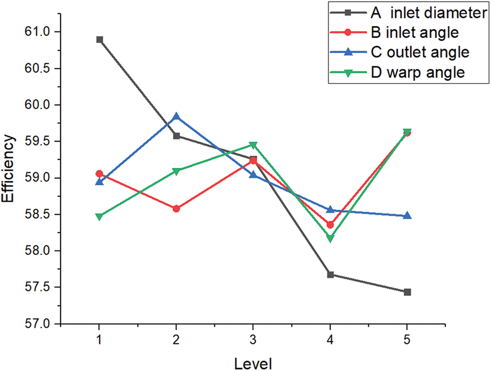
Figure 18: Line chart of influence of each factor on efficiency
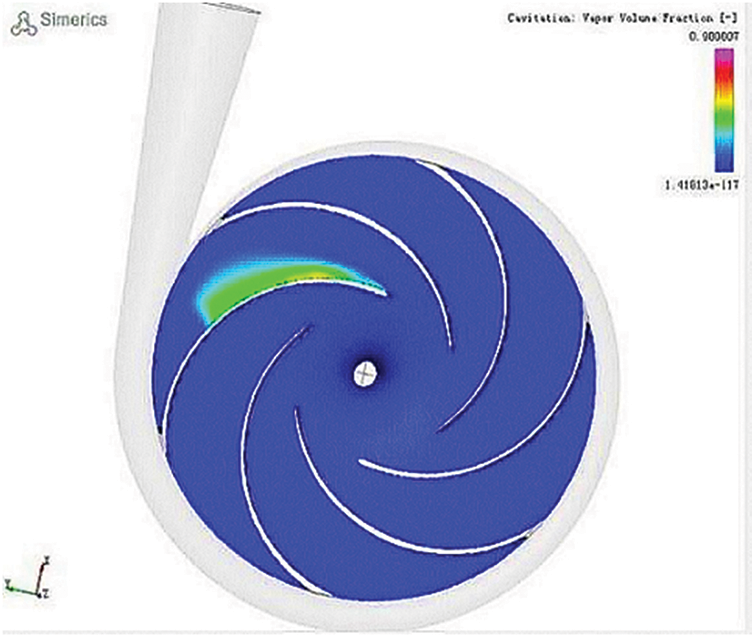
Figure 19: Vapor volume fraction (maximum efficiency)

Figure 20: Contour of velocity (maximum efficiency)
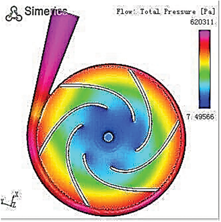
Figure 21: Contour of pressure (maximum efficiency)
By analyzing the result of the orthogonal experiment with the range method, the influence trend of each factor on each evaluation index was obtained as inlet diameter > wrap angle > outlet angle > inlet angle.
5 Optimization of the Impeller Parameters of the Plastic Centrifugal Pump Based on the Taguchi Algorithm
5.1 Determination of the Target Value
In light of the influence of pump efficiency and cavitation factors and the efficiency required for the plastic centrifugal pump in this work, the efficiency and cavitation were taken as evaluation indices to inspect the comprehensive performance of the plastic centrifugal pump. The proportion of cavitation was set to be 30% and the efficiency 70%.
5.2 Determination of the Controllable Factors and Levels
Comprehensively considering the efficiency of the plastic centrifugal plump and the cavitation, the four structural sizes: the impeller’s inlet diameter, inlet angle, outlet angle, and the wrap angle, were selected as the experimental factors. The factors were set at five levels, and the controllable factors and their levels were determined as shown in Table 2.
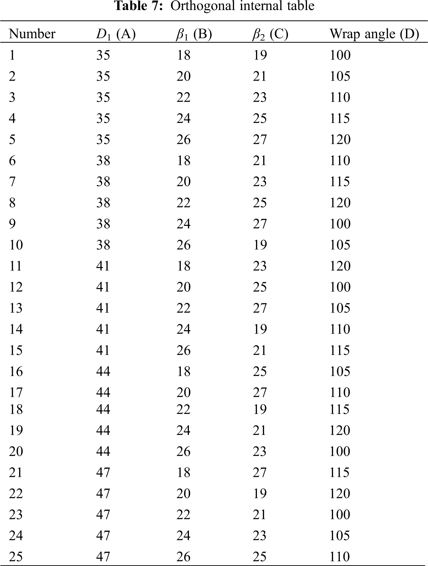
(1) The orthogonal internal table L25 (54) was selected as shown in Table 6. The interaction between factors was not considered because the following experiment index was SN ratio instead of quality characteristics [15].
(2) Calculation of SN ratios
The NPSH index in the software was the volume fraction of steam. In practice, a smaller or even zero value is better. In the Taguchi method, it is called the smaller-the-better type characteristic Yi, and its SN ratio can be calculated from Eq. (21):
Higher efficiency is better. In the Taguchi method, it is called the larger-the-better characteristic Yj, and its SN ratio can be calculated from Eq. (22):
Synthetic signal to noise ratio SN:
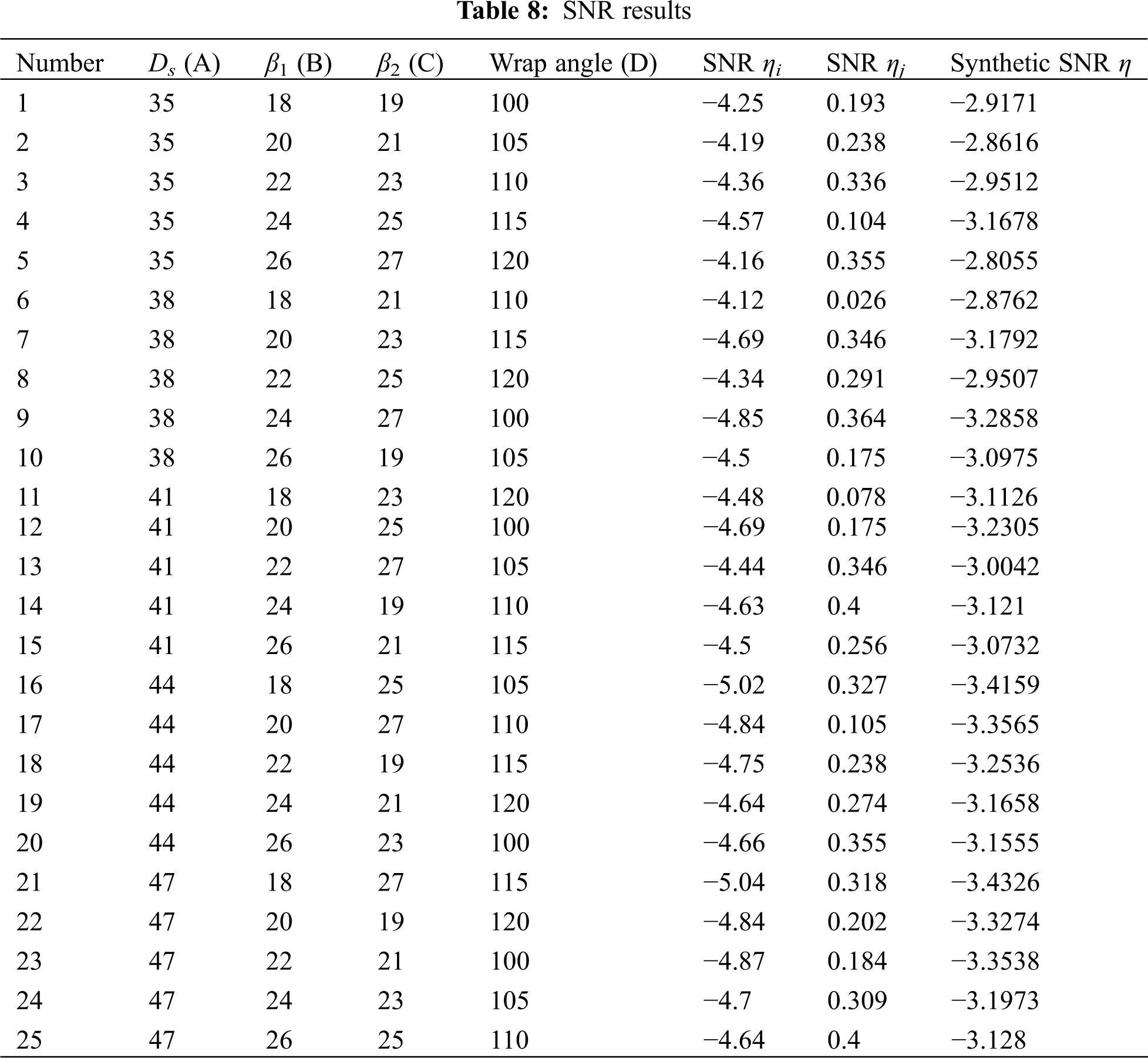
The result of SNR calculations is presented in Table 7.
According to direct analysis of Table 7 [16], the signal-to-noise ratio of the fifth group in the experiment is the largest at −2.8489, and the corresponding process parameter is A1B5C5D5.
(3) Statistics of the internal table [17]
①The sum of the SN ratios T can be calculated from:
Then,
②Under each factor lever, the sums of the SN ratios Ti, the mean values of the SN ratios ti, and the ranges of each column Ri were calculated, wherein i = 1, 2, 3, 4, 5. Results are shown in Table 8.
③The sum of squared total fluctuations of the SN ratios ST can be calculated from Eq. (25):
④The sums of squared total fluctuations of the SN ratios for each factor S1, S2, S3, and S4 [18] can be calculated from Eq. (26):
Then,
(4) Range analysis
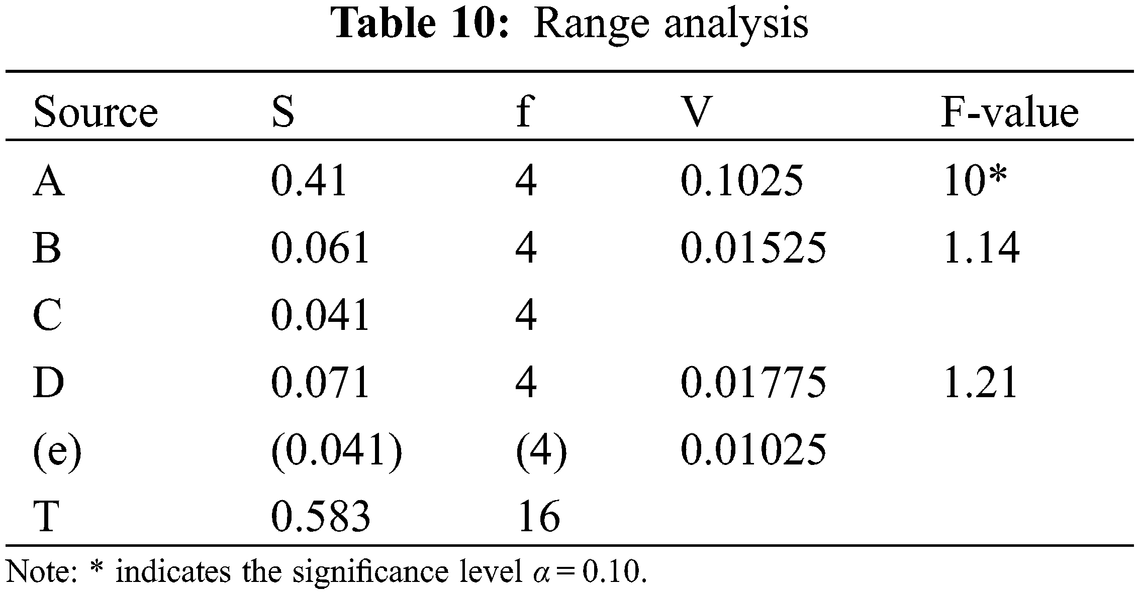
As there was no empty column in this experiment [19]; that is, there was no error term. Therefore, the smallest value S3 was taken as the sum of squared error fluctuations Se. Then,
The range analysis is shown in Table 9.
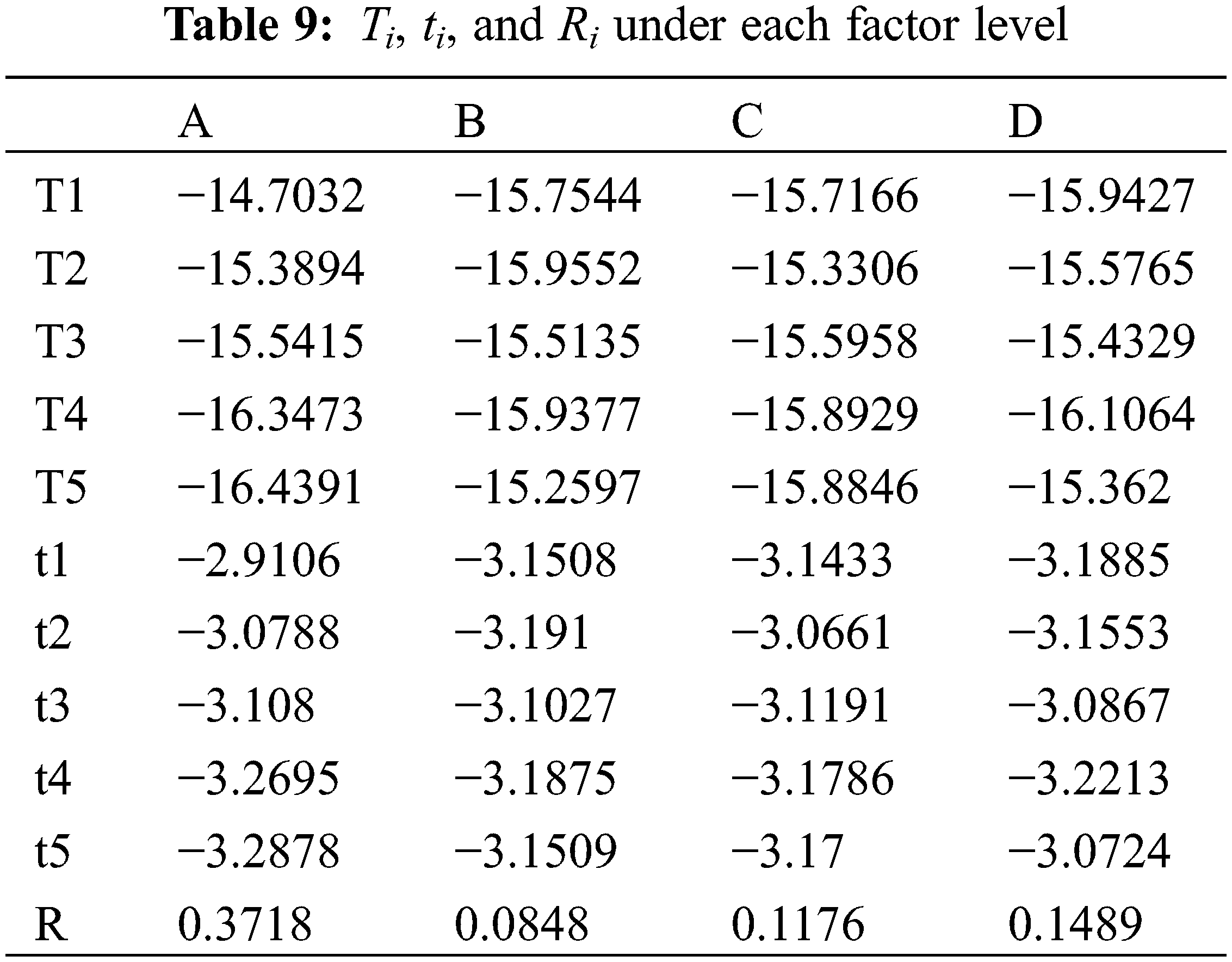
As per the range analysis of the signal-to-noise ratios, factor A has a significant effect on the quality fluctuation characteristics. Factor A can be considered a stable factor, while factors B, C, and D adjustable factors. For the stable factor, the level of factor A is A1. The vapor volume fraction signal-to-noise ratio ηj of factors B, C, and D are listed in Table 10.
As factors B, C, and D have little influence on the quality fluctuation characteristics, it is possible to neglect the efficiency and then adjust them until the vapor volume fraction reaches the minimum. As shown in Table 11, when only vapor volume fraction is considered, the optimum process parameters were B5C5D3.
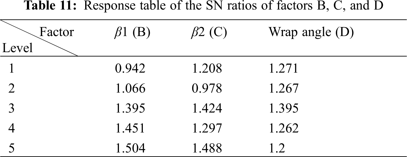
The optimal combination is A1B5C5D3, which is almost the same as the results from the direct analysis.
The impeller model was set to the following parameters:
Inlet diameter 35 mm, inlet angle 26°, outlet angle 27°, and wrap angle 110°.
After these parameters were imported into pumplinx, the simulation was performed thrice. The results are displayed in Table 12:
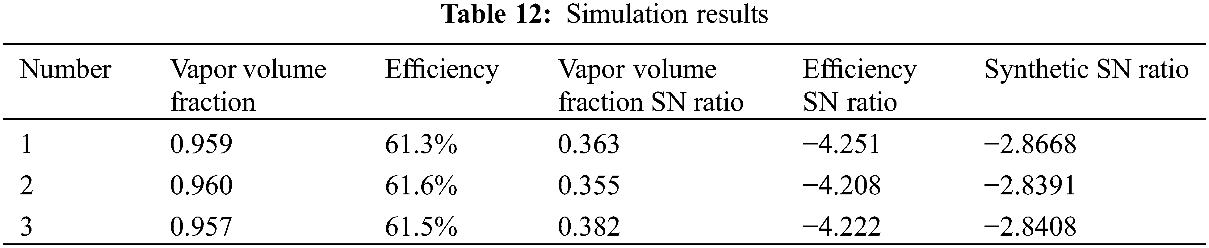
The synthetic signal-to-noise ratio obtained by the simulation with the optimized parameters was rather close to the synthetic signal-to-noise ratio of the fifth group, suggesting that the optimized parameters were reasonable.
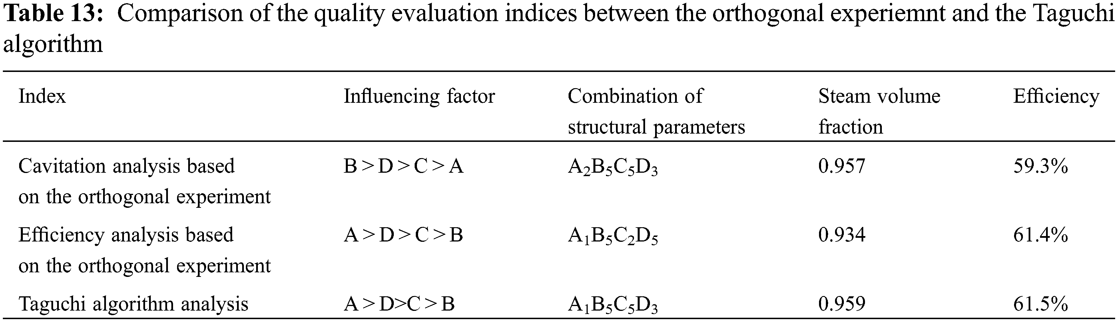
The molding process parameters were optimized by the orthogonal experiment and the Taguchi algorithm, respectively. Results were compared in Table 13.
It can be seen from Table 13 that with the orthogonal experiment and Taguchi algorithm to analyze and optimize the structural parameters of the centrifugal pump, different values of the quality indices are obtained. The steam volume fraction and efficiency obtained by the Taguchi algorithm are not optimal among the above three sets of quality evaluation indices, but both the steam volume fraction and efficiency are optimized. Therefore, it can be concluded that the Taguchi algorithm helps optimize the structural parameters of the centrifugal pump.
In this paper, CFD simulations were used to analyze the flow field of a plastic centrifugal pump. Through an orthogonal experiment and range analysis, the optimized parameters were obtained with efficiency and NPSH as the evaluation indices. With the maximum efficiency and minimum NPSH as evaluation indices for combination parameters, the Taguchi algorithm was employed to optimize the parameters of the plastic centrifugal pump to obtain the optimal combination parameters of the maximum efficiency and minimum NPSH.
(1) The structural parameters of the plastic centrifugal pump were calculated, modeled, and the flow field simulation analysis of the model was performed by CFD.
(2) Herein, an orthogonal experiment was designed and performed. Each factor affected the efficiency of the plastic centrifugal pump orderly by the impeller’s inlet diameter D1, wrap angle φ, outlet angle β2, and inlet angles β1. Each factor affected the cavitation of the centrifugal pump orderly by the impeller’s inlet angle β1, wrap angle φ, outlet angle β2, and inlet diameter D1.
(3) With the efficiency and cavitation of the plastic centrifugal pump as the evaluation indices, with the help of the Taguchi algorithm, the parameters of the impeller of the plastic centrifugal pump were optimized. The optimal combination parameters with the maximum efficiency and minimum cavitation were obtained as follows: The impeller’s inlet diameter D1 was 35 mm, inlet angle β1 26°, outlet angle was 27°, and wrap angle φ 110°. Then, the efficiency of the plastic centrifugal pump was highest, and cavitation lowest.
Funding Statement: This article belongs to the project of the “The University Synergy Innovation Program of Anhui Province (GXXT-2019-004)”.
Conflicts of Interest: The authors declare that they have no conflicts of interest to report regarding the present study.
1. Zhang, K. (2000). Principles of fluid machinery, vol. 1. China: Machinery Industry Press. [Google Scholar]
2. Mou, J. G., Shi, Z. Z., Gu, Y. Q., Wang, H. S., Zhao, L. P. et al. (2019). The influence of blade wrap angle on the cavitation performance of centrifugal pump. Journal of Zhejiang University of Technology, 47(1), 24–28. [Google Scholar]
3. Fu, Y. X., Yuan, S. Q., Yuan, J. P., Zhou, B. L., Wang, P. (2015). The effect of the number of blades on the cavitation characteristics of centrifugal pumps under small flow conditions. Transactions of the Chinese Society of Agricultural Machinery, 46(4), 21–27. DOI 10.6041/j.issn.1000-1298.2015.04.004. [Google Scholar] [CrossRef]
4. Wang, Q. L., Lv, H. X. (2016). Exploration and research on anti-cavitation measures for cryogenic liquid centrifugal pumps in air separation units. Cryogenics and Superconductivity, 44(8), 19–21+26. DOI 10.16711/j.1001-7100.2016.08.005. [Google Scholar] [CrossRef]
5. Lu, J. Y., Xu, W. Q., Zhang, Y. L., Li, L. H., Dou, H. S. (2021). The effect of the installation angle of the volute septum on the characteristics and flow stability of the centrifugal pump. Journal of Zhejiang Sci-Tech University (Natural Science Edition), 45(3), 351–364. DOI 1673-3851(2021)05-0351-14. [Google Scholar]
6. Guan, T. Y., Liu, X., Wang, J., Wang, Z. X., An, X. M. (2016). The influence of the area ratio of the inlet and outlet of the impeller channel on the performance of ultra-low specific speed centrifugal pumps. Shenyang Municipal Committee of the Communist Party of China, Shenyang Municipal People’s Government, Chinese Agricultural Society, 2016, 936–940. [Google Scholar]
7. Li, X. R., Zhu, B. S., Li, Z. G., Wang, W. J. (2021). Influence of blade wrap angle on hydraulic characteristics of double volute centrifugal pump. Thermal Energy and Power Engineering, 36(3), 35–42+105. DOI 10.16146/j.cnki.rndlgc.2021.03.005. [Google Scholar] [CrossRef]
8. Liu, Y. N. (2020). Research on the influence of blade curvature radius change on hydraulic performance of centrifugal pump impeller (Ph.D. Thesis). Lanzhou University of Technology, China. [Google Scholar]
9. Li, G., Sun, L., Wang, Z., An, C., Guo, C. et al. (2021). Investigation on the changing characteristics of flow-induced noise in a centrifugal pump. Fluid Dynamics & Materials Processing, 17(5), 989–1001. DOI 10.32604/fdmp.2021.016507. [Google Scholar] [CrossRef]
10. Tian, P., Huang, J., Shi, W., Zhou, L. (2019). Optimization of a centrifugal pump used as a turbine impeller by means of an orthogonal test approach. Fluid Dynamics & Materials Processing, 15(2), 139–151. DOI 10.32604/fdmp.2019.05216. [Google Scholar] [CrossRef]
11. Bai, Z. W., Pei, J. H., Hu, S. H. (2009). Numerical simulation machine of flow field in centrifugal pump. Mechanical Design and Manufacturing, 6, 223–225. DOI 10.3969/j.issn.1001-3997.2009.06.086. [Google Scholar] [CrossRef]
12. Barbarelli, S., Amelion, M., Florio, G. (2016). Predictive model estimating the performances of centrifugal pumps used as turbines. Energy, 107, 103–121. DOI 10.1016/j.energy.2016.03.122. [Google Scholar] [CrossRef]
13. Lian, S. J., Ma, G. C., Chen, W. H. (2014). Research on numerical simulation of full flow field of centrifugal pump based on CFX. Mechanical and Electrical Technology, (5), 32–33. [Google Scholar]
14. Pei, J. (2013). Transient hydraulic excitation of centrifugal pump, fluid-solid coupling mechanism and unsteady flow strength research (Ph.D. Thesis). Jiangsu University, China. [Google Scholar]
15. Fu, S. Q., Fang, S. J., Wang, Z. M. (2012). GPS microstrip antenna simulation design based on Taguchi optimization method. Journal of Microwaves, 28(3), 33–38. DOI 10.14183/j.cnki.1005-6122.2012.03.013. [Google Scholar] [CrossRef]
16. Du, G. S., Li, D. X. (2004). Tian Tue experiment set up juice method to optimize the column chromatography separation process of TPGS mono- and di-vinegar. Chemical Reagents, 36(1), 79–81. DOI 10.13822/j.cnki.hxsj.2014.01.020. [Google Scholar] [CrossRef]
17. Hu, B., Zhang, Q. W., Zhao, X. (2010). Research on optimization design of CRT thermal explosion cutting equipment based on Taguchi method. Chemical Machinery Design and Manufacturing, 5, 15–17. DOI 10.3969/j.issn.1001-3997.2010.05.006. [Google Scholar] [CrossRef]
18. Zheng, J., Cheng, A. G., Dong, L. Q. (2011). Application of Taguchi robust design method in the optimization of automobile crashworthiness. Auto Wangcheng, 33(9), 772–776. DOI 10.19562/j.chinasae.qcgc.2011.09.008. [Google Scholar] [CrossRef]
19. Ding, W. H., Qian, Z. (2007). Research on optimization of wood products numerical control processing parameters based on Taguchi method. Wood Processing Machinery, 6, 15–18. DOI 10.3969/j.issn.1001-036X.2007.06.002. [Google Scholar] [CrossRef]
 | This work is licensed under a Creative Commons Attribution 4.0 International License, which permits unrestricted use, distribution, and reproduction in any medium, provided the original work is properly cited. |