Fluid Dynamics & Materials Processing

DOI: 10.32604/fdmp.2022.018841

ARTICLE

Numerical Investigation into the Transient Behavior of the Spike-Type Rotating Stall for a Transonic Compressor Rotor

Pengfei Ju1,2, Fangfei Ning3,4,*, Zhiting Tong1,2 and Jingying Wang5,6

1Tianjin Key Laboratory for Advanced Mechatronic System Design and Intelligent Control, School of Mechanical Engineering, Tianjin University of Technology, Tianjin, 300384, China
2National Demonstration Center for Experimental Mechanical and Electrical Engineering Education (Tianjin University of Technology), Tianjin, 300384, China
3Research Institute of Aero-Engine, Beihang University, Beijing, 100191, China
4National Key Laboratory of Science and Technology on Aero-Engine Aero-Thermodynamics, School of Energy and Power Engineering, Beihang University, Beijing, 100191, China
5School of Energy and Power Engineering, Shandong University, Jinan, 250061, China
6Shandong Engineering Laboratory for High-Efficiency Energy Conservation and Energy Storage Technology & Equipment, Shandong University, Jinan, 250061, China
*Corresponding Author: Fangfei Ning. Email: fangfei.ning@buaa.edu.cn
Received: 20 August 2021; Accepted: 13 December 2021

1  Introduction

The rotating stall phenomenon has been studied for decades, especially spike-type stall has been discovered for nearly 30 years [1,2]. Spike stall was originally called “short length scale disturbance”, which was first reported by Day [3], and was then distinguished from the other kind of “modal stall” [4]. Spike stall has the following characteristics: (1) The spike precursor is a small-scale disturbance, which starts with a sudden small spike in the dynamic signal (the modal type starts with a gradually increasing low-order modal disturbance). (2) The development period of spike stall is short, which takes 2–3 revolutions from the appearance of the first spike to full development of stall cells (while the development period of modal wave is about 50 revolutions). (3) Spike precursor only appears in the tip region (modal wave can be detected in the whole blade height). According to the flow field results of previous numerical studies, several flow structures corresponding to spike precursors have been proposed, such as leading edge spillage [5–7], tornado vortex [8], and leading edge separation vortex [9], etc. However, there have been few conclusions on stability mechanism besides flow structures.

The abruptness of spike stall shortens the stall warning time to merely 2 revolutions, which makes it very difficult to implement active control methods, especially for high-speed compressors [10–12]. The actuator often needs a certain amount of time to influence the flow field in the channel, so it is best to warn before the flow field deteriorates seriously, in which sense spike signal appears too late. In fact, some special unsteady flow phenomena have been reported under near-stall conditions, such as bubble-type breakdown and spiral-type breakdown of the tip leakage vortex [13,14], self-induced unsteadiness [15], rotating instability [16,17], and periodic shedding of leakage vortex [18], etc., which are also considered to be related to stall. However, when these phenomena occur, the compressor itself can still operate stably, so they cannot be considered as the leading event of spike, and it is too conservative to trigger the flow control mechanism based on them.

There are many difficulties in detecting the early signal characteristics ahead of the spike. In experiments, the dynamic probe signals installed on the casing need to filter out the blade passing frequency (BPF) to identify the stall inception, due to the strong deterministic disturbance caused by blade sweeping. Additionally, with the influence of noise, any short scale features earlier than spike have not been identified. In simulations, spike feature is often triggered by artificial disturbance due to the limitation of CPU time, which covers up the potential inherent instability in the flow field. The post-spike process has been fully studied, while few case studies has been carried out in the pre-spike phase.

The numerical simulation of rotating stall process for NASA37 transonic compressor rotor has been carried out in a previous study by the authors. In addition to the common development process of spike disturbance which has been reported, this simulation also retains some information of flow behavior ahead of spikes by avoiding any artificial interference. The present paper will focus on the flow field characteristics and signal characteristics before spike appears, and also discuss the effectiveness of the identification method on this early disturbance.

2  Brief Introduction of Examples and Methods

2.1 Testing Case

The object of this study is NASA Rotor 37 transonic compressor rotor, designed by NASA Lewis Research Center in 1978 [19], and was used as a challenging test case of ASME International Gas Turbine Institute (IGTI) for verification by many numerical simulation programs [20]. The rotor has 36 blades, with aspect ratio 1.19, hub ratio 0.7, tip tangent velocity 454 m/s, multi-arc blade profile, tip solidity 1.29, design equivalent flow rate 20.19 kg/s and design total pressure ratio 2.1.

2.2 Numerical Method

An in-house program for numerical simulation of turbomachinery three-dimensional flow field, named MAP (Multi-block Aerodynamic Prediction code), is used in the present study. It is a Finite Volume Method (FVM) Raynolds-Averaged Navier-Stokes (RANS) solver, and supports GPU (Graphics Processing Unit) acceleration. After years of application, it has been well verified and function extended. This code is specifically described in detail in the literature [21]. MAP solves the integral form of governing equations (including one density equation, three momentum equations, one energy equation, and one or more turbulence model equations) based on the cell-centered finite volume method. The advective flux is discretized by LDFSS scheme [22] which is one of the AUSM-family schemes and performs quite well in the viscous and shock wave containing flows. The MUSCL interpolation with minmod limiter is applied to approach high order of spatial accuracy and ensure monotone solutions near discontinuities. For the discretization of diffusive flux, the traditional 2nd-order central differencing is used. For the steady flow simulation or the inner loop of the dual time stepping time-accurate simulation [23], the time derivatives are discretized by 1st-order Euler backward scheme, which finally forms an implicit linearized system and is solved by the LU-SGS method. The physical time derivatives are discretized by 2nd-order Crank-Nicolson scheme. Considering the requirements of numerical stability and time resolution, each blade passing period includes 50 physical time steps, and the inner loop includes enough pseudo time steps to ensure convergence (The residual drops by three orders of magnitude). A modified S-A (Spalart-Allmaras) turbulence model is adopted in this case. With the help of GPU acceleration technology, this simulation is carried out on a workstation with four GPUs, which can simulate one rotation of the rotor in about 3.5 days.

2.3 Grid and Computational Domain

Fig. 1 gives diagrams of the whole ring computational domain and the computing mesh. The structured mesh was generated by another in-house code and adopted an O-3H topology in the blade passage and an O-2H topology in the tip clearance region respectively. In order to prevent the inlet and outlet boundary conditions from influencing the free growth of circumferential low-order perturbations, the spaces upstream and downstream of the rotor were extended by a length of rotor diameter respectively. The total number of grid points is about 24 million, among which there are about 570 thousand fine grid points around each blade (with approximately 71 × 81 × 64 grid points in spanwise, chordwise and pitchwise directions, respectively). In the practice of the MAP program with S-A model, y+ = 5 is an optimized value, which was also adopted in this case.

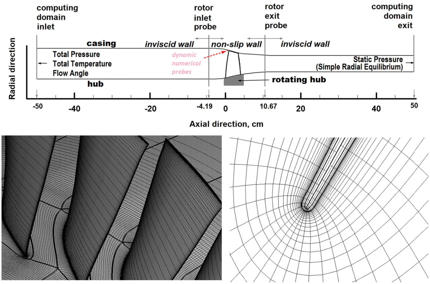
Figure 1: Computational domain and computational grid schematic

2.4 Boundary Conditions

The circumferential uniform total temperature, total pressure and axial airflow direction are set at the inlet boundary, whose values are coherent with the test data. The outlet circumferential uniform static pressure was defined with the casing pressure fixed, which accords with a simple radial equilibrium relationship. Other boundaries are viscid or inviscid walls. In order to mitigate the interference caused by the extension of the computational domain upstream and downstream, inviscid walls were adopted in areas beyond the two probing stations of the test. The outlet casing static pressure remained constant at the initial stage of calculation, and then was controlled by a throttling model after the stall precursor became significant (the moment was about 5.5 revolutions) to avoid excessive decrease of the mass flow. In this throttling model, the static pressure difference across the outlet boundary is proportional to the quadratic of the mass flow.

3  Results

3.1 Brief Introduction of Stall Process

Before the full annulus calculation starts, steady single passage calculations were carried out with periodic boundary conditions to obtain the results of operating characteristics, which well matches with the test results, as shown in Fig. 2. The mass flow has been normalized according to the test chocking flow rate (20.93 kg/s). The calculated mass flow rate at the near stall condition is about 0.932, while the experimental value is 0.928. The calculated total pressure ratio is very close to the experimental curve, whereas the efficiency is slightly underestimated. The unsteady single passage calculations were carried out at several operating points, and the long-time converged results were also consistent with the steady calculation results. At the near-stall point, an additional continuous calculation of about 20 revolutions was carried out after the flow rate became stable, and the flow rate remains constant except for a slight periodic fluctuation. This flow field was used as the initial field of the full annulus calculation after replicating to 36 channels.

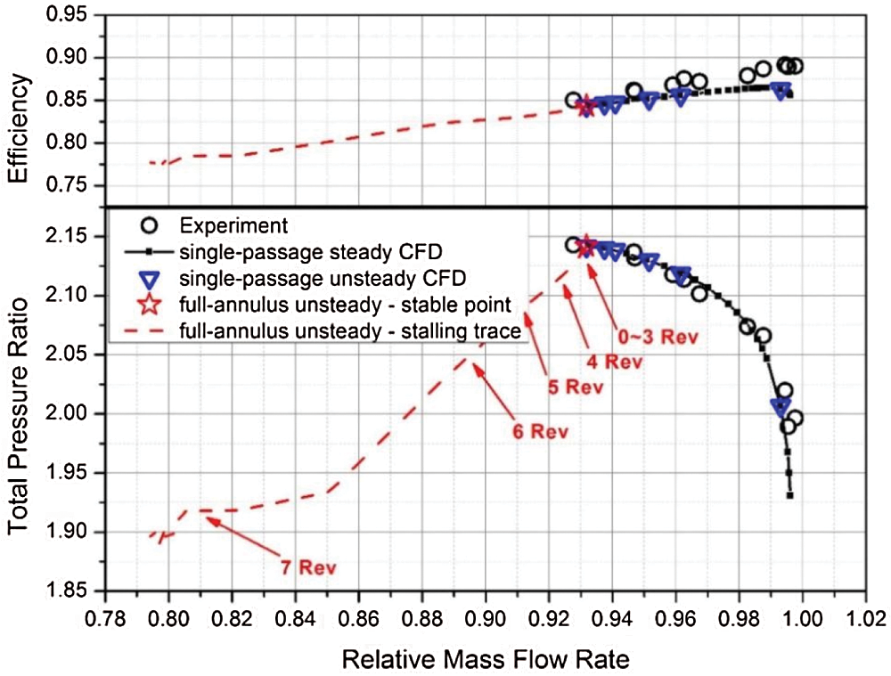
Figure 2: Operating characteristics and stall trajectory from experiment and CFD results

As mentioned above, the outlet casing pressure remained the same as that in single passage calculation at the initial stage of the full annulus calculation, while the whole ring flow failed to maintain stable. Fig. 3 shows the flow rate trajectory of the full annulus calculation compared with the single channel calculation result. It can be seen that the flow rate begins to drop significantly at about 4 revolutions after switching to full annulus calculation. Finally, the relative flow rate of stable stall state is about 0.8 with the restriction of the throttling model. The stall inception is spike-type. The initial three spikes and relevant leading edge spillage characteristics are found between 5–5.5 revolutions, and then develop into three stall cells in the following 2 revolutions. More details about the spike-type inception and the developing process of stall cells in this result can be found in literature [24]. The present paper focuses on the flow behavior before spike signal appears, which is rarely mentioned in previous studies so far.

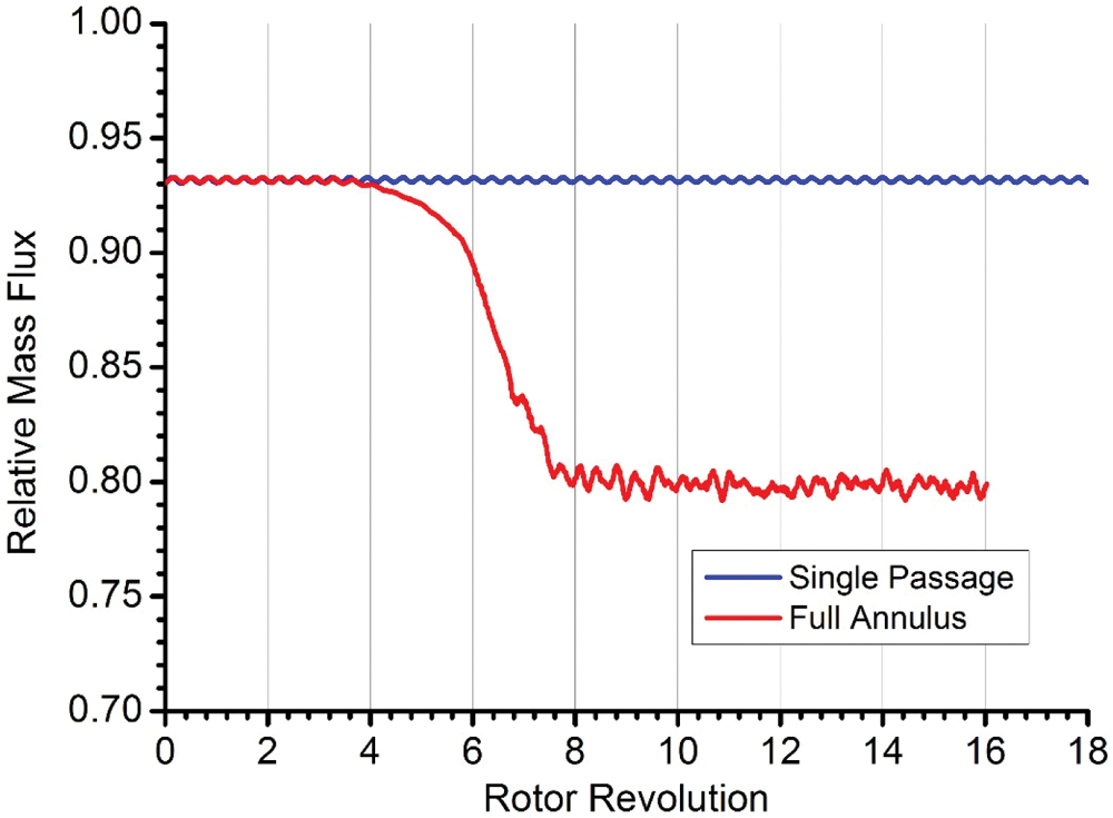
Figure 3: Mass flow rate history in single-passage and full-annulus calculations

3.2 Unsteady Behavior of Flow Fluctuation

It can be seen from Fig. 3 that there is a periodic flow fluctuation in the flow field before the flow rate drops sharply, and its period is about 0.35 revolution. Fig. 4 shows the spanwise distribution of the circumferential averaged axial velocity deviation obtained from the sections of the inlet and outlet planes of the rotor at different moments in a cycle. It can be seen that the deviation direction on the whole spanwise region is approximately the same at the inlet section, while the tip part varies slightly earlier than the root part.

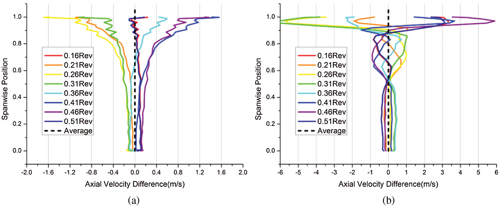
Figure 4: Spanwise distribution of axial velocity at rotor inlet and exit sections (Axial gap of 0.1 chord) (a) Inlet section (b) Exit section

At the exit section, the deviation directions at different spanwise positions are inconsistent, and the fluctuation amplitudes are also different. At 50% span and 90% span, there are regions with minimal amplitude, and the whole spanwise space can be divided into three regions by them. The upper region has the largest amplitude (up to 6 m/s), and the deviation direction in the whole region is basically the same. The amplitude in the middle region is about 1 m/s, but the internal fluctuations are asynchronous and show the form of propagating upwards. The amplitude of the lower region is about 0.5 m/s, and the overall trend is basically synchronous. The phase of the lower region is close to that of 80% span and 1/4 cycle slower than that of 60% span.

This periodic fluctuation can also be discovered from the flow distribution at the exit plane of the rotor. Fig. 5 shows the axial velocity distribution on a plane at 90% axial position of the tip chord near the outlet of the blade passage. It clearly shows that the blockage in the blade passage includes two parts: the blockage related to boundary layer separation on the suction surface of the blade and the blockage related to leakage flow on the end wall. The blade surface separation is mainly distributed in the part above 50% span, and the thickness distribution of the blocking area is different at different moments. At the moments of 0.36 revolution and 0.41 revolution, the boundary layer mainly thickens in the region of 60%∼80% span, and then the blockage gradually extended to the tip corner region and the end wall (at the moment about 0.21 revolution). With the blockage transferred to the end wall, the boundary layer thickening on the suction surface gets alleviated again.

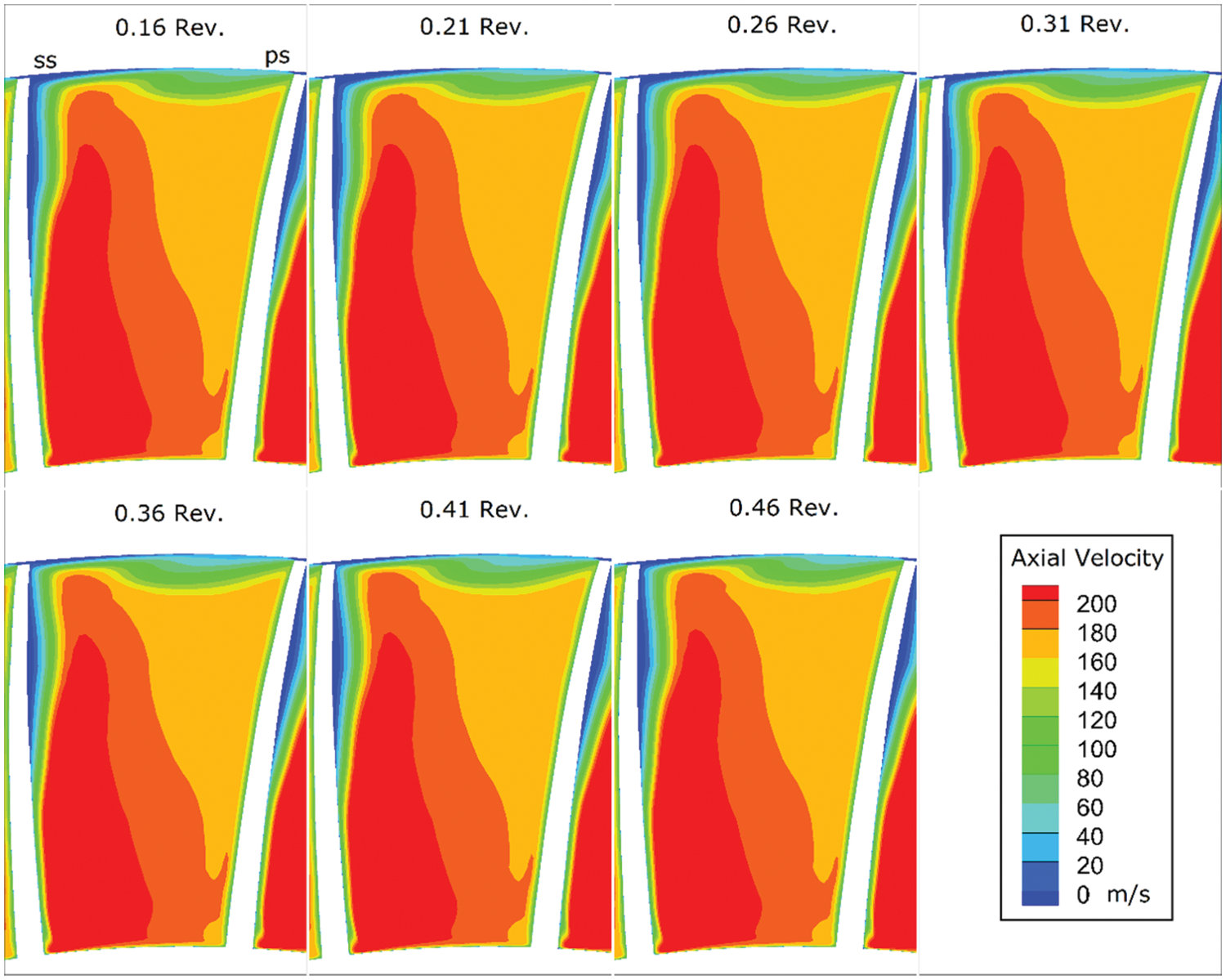
Figure 5: Axial velocity on the plane near the rotor exit (90% tip axial chord position)

Generally speaking, the flow blockage is generated and accumulated on the blade suction surface, and periodically offloaded to the end wall along with the secondary flow (The spanwise transport of secondary flows is a relatively common phenomenon, such as literature [25]). In particular, the blockage at 50%∼90% span is mainly contributed by the boundary layer separation which transfers periodically along the radial direction on the blade surface. This explains why the middle region in Fig. 4b shows the pattern of propagation upwards.

3.3 Unsteady Signal Characteristics

The stall signal corresponding to the test results can be obtained from the “numerical probes” set on the casing in front of the rotor. Fig. 6 shows the static pressure signals in the first 10 revolutions of the full annulus calculation. These six numerical probes evenly arranged in the circumferential direction were set on the casing in front of the rotor with a distance of 0.1 times axial chord length from the leading edge of the rotor, and were stationary relative to the ground. The signals of the six probes “fixed” in the stationary frame were rebuilt from data of hundreds of interpolated sample points in the computational grid. The original signal and the low-pass filtered signal are shown in Fig. 6, in which the SINC filter with Blackman window is used for the low-pass filtering treatment with the cut-off frequency 0.75 BPF and the transition bandwidth 0.11 BPF, which can effectively remove the deterministic disturbance of blade sweeping and retain the influences of cross-channel flow structures.

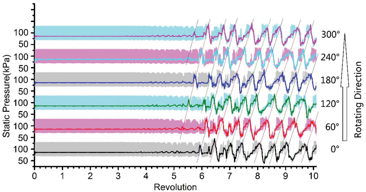
Figure 6: Static pressure signals from six upstream probes fixed on the casing (Axial gap of 0.1 tip axial chord, before and after low-pass filter, cut-off frequency 0.75 BPF, transition bandwidth 0.11 BPF)

Three spike-type perturbations occur between 5.5 and 6.0 revolution moments. They eventually develop into three stall cells at about the 7.5 revolution moment. Between 6.0 and 7.5 revolution moments, significant amplification and deformation occurs in these three spike disturbances, and some small spike-like disturbances are separated from the major disturbances and finally disappear. After the 7.5 revolution moment, the signal characteristics of the three stall cells also become stable along with the stabilization of rotor flow rate, which moves along the circumferential direction at the speed of about 62.5% rotor speed. These characteristics are consistent with the results of numerous previous experimental and computational studies.

It is significant to find out that there have been a lot of small amplitude disturbances in the filtered signal within 2 revolutions before the first spike precursor appears. These early disturbances show no regular pattern, and their amplitudes increase slowly. In experimental studies, this irregular small-amplitude disturbance can be easily confused with the measurement noise. In the present study, there are merely long-period circumferential-uniform weak fluctuations in the early stage due to the absolute uniformity of initial conditions, boundary conditions and geometric conditions. Therefore, it can be concluded that this feature of irregular small “early disturbances” is part of the entire stall development process, and it is a remarkable unsteady feature ahead of the spike-type disturbance.

Fig. 7 shows the amplitude spectrum of spatial Fourier transform of circumferential pressure distribution in the first 10 revolutions, and the color represents the logarithm of amplitude. The position of the probe set is mentioned above. It can be seen that the 4th and 5th harmonic disturbances appear and develop slowly between 3–3.5 revolution moments. At the 5.0 revolution moment, the strongest harmonics are the 3rd and 4th components, while the amplitude increases little. At about 5.5 revolution moment, almost all the harmonics increase at the same time, which accords with the characteristic of a circumferential impulse, and corresponds to the appearance of the first spike disturbance. At the 6 revolution moment, the amplitude of the 3rd harmonic increases significantly with the development of the three major spike disturbance.

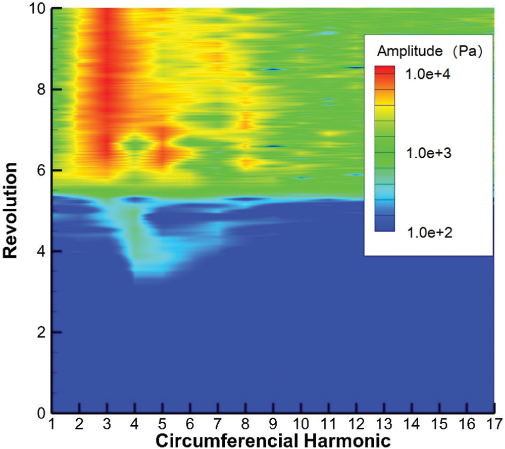
Figure 7: Amplitude spectrum of spatial Fourier transform of circumferential pressure distribution (Casing static pressure, 0.1 tip axial chord ahead of the leading edge)

Fig. 8 shows the temporal and spatial distribution of the disturbance, which is also sampled at the inlet casing of the rotor, but the probe set is fixed in the rotor frame with 360 probes. It is obvious to notice that at the time of near the 6 revolution, three spike perturbations appear and start propagating in the contrarotating direction. However, between 3.5 revolution and 5.5 revolution moments, there are some disturbances with small amplitude, and they propagate forward along the rotor rotating direction even in the rotor frame. There are about four of these strip-shaped early disturbances propagating forward (with another shortly appeared one not included here), which are not completely uniform in the circumferential direction, and the widths of each strip are also different. Then three spike perturbations originate from the strip and propagate back at the meantime, while the early disturbances gradually disappear. Thanks to the absence of deterministic disturbances in the rotor frame, these weak early disturbances can be clearly detected. However, they only appear at a specific position of each rotor channel. On the contrary, when the spike disturbance occurs, the pressure variation extends to a large area in the blade passage.

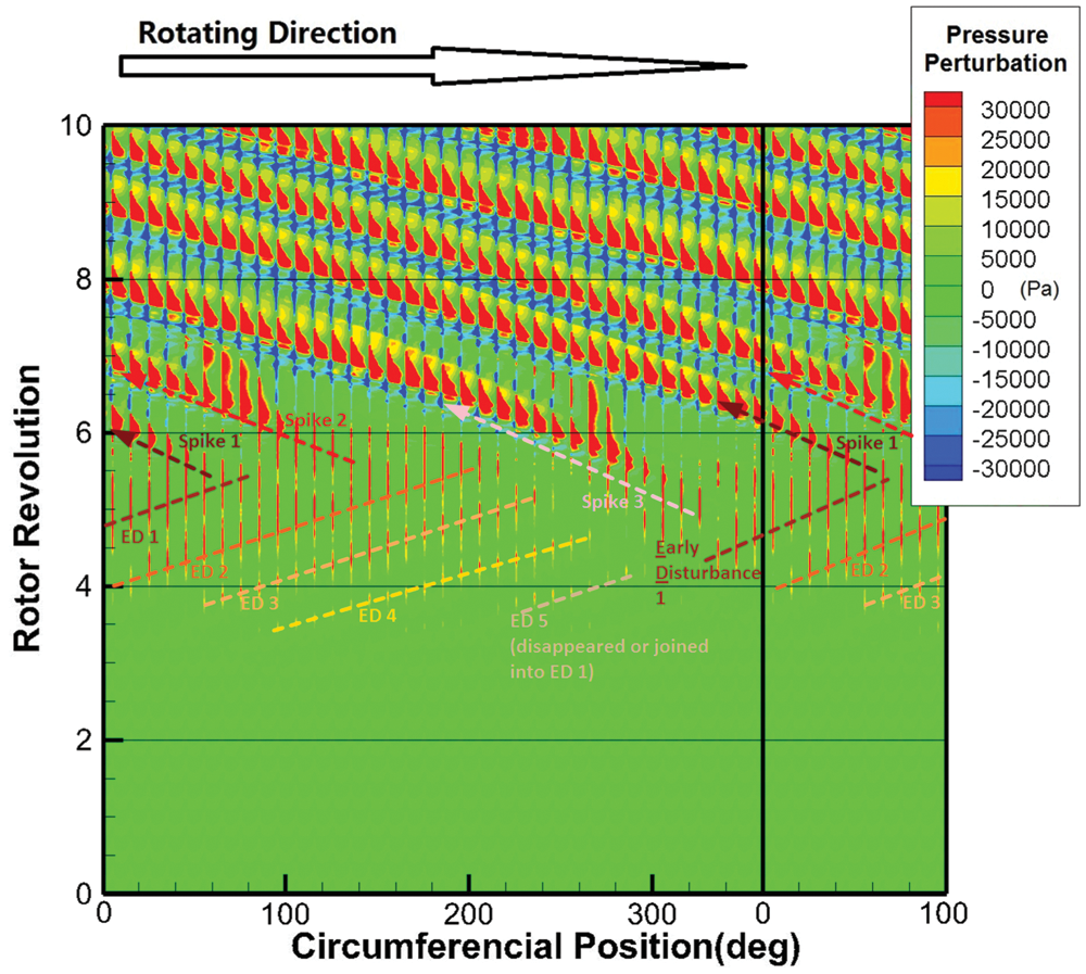
Figure 8: Spatio-temporal pattern of pressure perturbation in rotating frame (Directly sampled from 360 monitor points in the computing grid, sampling location the same as the figure above)

3.4 Recognizability in the Stator Frame

On test rigs, sensors are mostly installed on the casing, so it is of practical significance to observe the spatio-temporal pattern of disturbance propagation in the static reference frame, and the strong deterministic disturbance of blade passing frequency must be filtered out. By using appropriate circumferential offset at each time step, the temporal and spatial distribution of disturbance under “static probes” can be extracted from the calculation results, which is shown in Fig. 9 after low-pass filtering. The filter parameters are the same as those used in Fig. 6. Under the same coloring levels, the intensity of spike disturbance is well preserved in the stator frame, while the amplitude of early disturbance is significantly attenuated. However, from this perspective, spike perturbations appear to develop continuously from several strips of early disturbance. Fig. 9 is a more detailed version of Fig. 6. It shows that there are several weak disturbances moving beyond the rotor speed in the early stage, with the quantity varying in the circumferential motion. Then, three of them slow down with their amplitudes increasing, and develop into three spike disturbances afterwards, and eventually develop into stall cells.

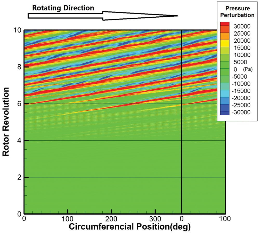
Figure 9: Spatio-temporal pattern of pressure perturbation in stator frame (Transformed from monitor point data of Fig. 8 and low-pass filtered)

The results of Fig. 9 were also converted into the rotating frame, as shown in Fig. 10. Due to the low-pass filter, the trace of each blade channel cannot be distinguished in Fig. 10 compared with Fig. 8, while the disturbance of large spatial scale is maintained. The main features of the three spike disturbances remain the same, and they become continuous strip pattern because the blade passage features have been filtered out, and their starting points become clearer. Early disturbances become difficult to recognize due to significant reduction in amplitude, but the pattern of disturbances is similar to that in Fig. 8, and the disturbances show forward propagation.

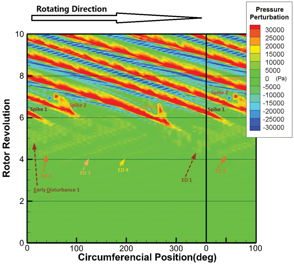
Figure 10: Spatio-temporal pattern of pressure perturbation in rotor frame, rebuilt from stationary frame low-pass filtered data (Transformed from data of Fig. 9)

4  Analysis

(1)   In the initial periodic fluctuation of the flow field, flow conditions on different spanwise location change periodically. This pulsation appears in both single-passage and full-annulus calculation, but it can keep its sustainability in single-passage calculation, while the full-annulus calculation finally develops into stall. It shows that the absence of forced circumferential uniformity is one of the key factors leading to the stall. The period of this fluctuation is about 12.6 times of the blade passing period, which is much longer than the typical period of pre-stall behavior mechanisms such as rotating instability [16,17] or self-induced unsteadiness [15]. This fluctuation shall not be classified into any known pre-stall behavior. Considering the flow field and flow distribution show the pattern that the blockage state transfers from the blade surface to the end wall, the secondary flow on the suction surface of the blade may play an important role in the propagation of the blockage state.

(2)   Spike signal is usually considered as the origin of the spike stall. However, in this study, we find that there are already early disturbances in the signal at 2 revolutions before spike feature appears, while its amplitude develops slowly, its distribution is nonuniform, and it propagates forward relative to the rotor. The development duration of early disturbance is similar to that of the spike, which should be considered as one of the important stages in the development of the stall. However, this stage has not been reported in any literature yet.

(3)   The flow rate of the whole machine decreases significantly since the 3.5 revolution moment, which is basically consistent with the moment when the early disturbance appears. The mass flow has been declining at an accelerating rate when spikes appear. Therefore, spike is not the reason for the drop of mass flow. On the other hand, since the flow rate cannot decrease indefinitely, the rotor will eventually reach the stall condition, and the appearance of spikes, which are the initial form of stall cells, should be regarded as an inevitable result of the flow rate decrease. The discussion of the spike stall mechanism should focus on the period at 3.5 revolution or earlier. In the present NASA Rotor 37 case, there is only circumferential uniform periodic fluctuation at the initial stage, and then early disturbances appear. The reason why the circumferential uniformity is broken needs more in-depth study.

(4)   The spatio-temporal pattern of the static pressure disturbance natively sampled in the rotor frame can well reflect the early disturbance. However, if sampled in the stator frame and low-pass filtered, the obtained amplitude of the early disturbance will be significantly reduced. This is because the early disturbance only concentrates in a specific position in each blade channel, and it comes from the waveform deformation of the deterministic blade sweeping disturbance in static probe signals, while the waveform can be attenuated by the low-pass filter. The retained amplitude is equivalent to the average of the amplitude of the most significant point in Fig. 8 across a blade passage, which seems also reasonable. However, it is unfavorable for recognizing the early disturbance. The severe change of pressure at the special position in Fig. 8 means the change of local flow structure, such as the movement of shock wave surface, which can only be captured at specific sampling positions. In experiment condition, the frequency response of the sensors must be high enough to precisely distinguish the position of the shock wave in order to achieve the effect like Fig. 8. Otherwise, the spatio-temporal pattern in rotor frame will show the effect similar to Fig. 10.

Moreover, when a spike appears, there is a great pressure deviation at most positions in the blade channel. This shows that the change of flow field structure is global instead of being local, and it also shows the degradation of blade working capability. This corresponds to the widely accepted flow features such as leading edge spillage and trailing edge backflow as well. In contrast, the early disturbance only represents the change of shock position, and there is no radical change in the working capability of the blade. Hence, it is easier to recover to normal working condition with the intervention of external force in the early disturbance stage than in the spike-type disturbance stage, which calls for an effective identification technology on early disturbance.

5  Conclusions

In the present paper, the rotating stall process of NASA Rotor 37 at design speed is studied numerically. Starting from the circumferential symmetric and stable operating initial field, the rotor flow field generates the spike-type stall inception without any artificial disturbance, and finally enters into a stable stall state. The early stage of stall process is analyzed, especially the behavior before the spike appears. The following conclusions deserve attention:

(1)   Spike is not the origin of the stall process, but an important milestone. It is at a mid-term position in the process of flow decrease.

(2)   The initial periodic fluctuation of the flow filed comes from the non-synchronous fluctuations at different spanwise locations. This kind of long-period fluctuations should not be classified into any known pre-stall behavior.

(3)   Before the first spike appears, there has been a set of early disturbances, whose amplitude increases slowly and propagates in the circumferential direction beyond the rotor speed. It is an earlier signal feature related to stall in dynamic probe signals than the spike disturbance.

(4)   In the present transonic rotor, large amplitude early disturbance can be detected at specific positions in the rotor frame, which reflects the movement of the shock wave surface. If the original signal is obtained by stationary mounted probes, the sensor system response frequency must be high enough, otherwise the early disturbance signal will be greatly attenuated.

In this example, the early disturbance feature can provide an extra 2 revolutions period in advance for stall warning, and keep the flow field structure almost unchanged during this period, and thus lead to a new possibility for active control of spike stall. More research is needed to effectively capture this early disturbance timely and separate it from deterministic BPF signal and background noise.

Funding Statement: This work was supported by the National Natural Science Foundation of China (No. 51976139), and the Shandong Provincial Natural Science Foundation, China (No. ZR2019QA018).

Conflicts of Interest: The authors declare that they have no conflicts of interest to report regarding the present study.

This work is licensed under a Creative Commons Attribution 4.0 International License, which permits unrestricted use, distribution, and reproduction in any medium, provided the original work is properly cited.