Fluid Dynamics & Materials Processing

DOI: 10.32604/fdmp.2022.019446

ARTICLE

An Improved Parameter Dimensionality Reduction Approach Based on a Fast Marching Method for Automatic History Matching

Hairong Zhang1, Yongde Gao2, Wei Li2, Deng Liu3,*, Jing Cao3, Luoyi Huang3 and Xun Zhong3

1Southern Marine Science and Engineering Guangdong Laboratory, Zhanjiang Bay Laboratory, Zhanjiang, 524000, China
2Zhanjiang Branch of China National Offshore Oil Corporation, Zhanjiang, 524000, China
3College of Petroleum Engineering, Yangtze University, Wuhan, 430100, China
*Corresponding Author: Deng Liu. Email: cjdxliudeng@163.com
Received: 25 September 2021; Accepted: 26 October 2021

1  Introduction

Reliable reservoir models can accurately reproduce the complete reservoir developing process and provide convincing guidance for production management decision-making [1–5]. History matching that can correct reservoir model parameters based on geological information and production data is a critical step in reservoir numerical simulation process. Traditional history matching methods are generally time-consuming, and the accuracy could hardly be guaranteed. In recent decades, automatic history matching methods has made great progress with improved optimization algorithms, in which case the model parameters would change automatically to minimize the difference between the established model and the real one. Currently, automatic history matching technology has become a hot research area in intelligent reservoir development.

Generally speaking, there is a close correlation between reservoir physical properties and well production performance, and history matching algorithms are mainly used to calculate the gradient and to direct the countermeasures. To the best of our knowledge, the widely used algorithms for history matching mainly include gradient-class method [6,7], set-class algorithm such as EnKF [8], ES-MDA [9] and SPSA [10], interpolation algorithms such as NEWUOA [11] and Wedge [12], and global optimization algorithms such as PSO [13] and GA [14]. The gradient-class method shows very high convergence rate, in which case, calculate the gradient of objective function or Hessian matrix is the key. However, there are also two limitations when using the gradient-class method for history matching: (1) gradient solving is difficult. The reservoir model usually contains hundreds of thousands of unknown parameters, which makes it impractical to store and calculate the sensitivity matrix. (2) pseudo correlation between real gradient and calculated gradient. The prior reservoir model based on scarce geological information is generally quite different from the real reservoir, which leads to inaccurate covariance between calculated production data and reservoir parameters. That means the calculated correlation between distant grids is large instead of small. As a result, the calculated gradient deviates seriously from the actual gradient.

In order to reduce the dimensionality of variables in the history matching, several parameterization methods were proposed. The overall idea is to convert the original high dimensional optimization problem to a low dimensional problem without changing the main features. The parameterization methods mainly include principal component analysis (PCA) method [15–18], Karhunen-Loeve (K-L) decomposition method [19], gradual deformation method (GDM) [20], pilot point method [21], discrete cosine transformation (DCT) method [22–24] and so on. PCA is a statistical analysis method, which is widely used in areas such as finance [25], machine learning [26] and so on. This method adopts orthogonal transformation to linearly transform the observed values to a series of possibly related variables, so as to project them into the values of a series of linearly uncorrelated variables. These unrelated variables are called principal components. In the oilfield, PCA method is commonly applied to extract reservoir heterogeneity and to reduce the calculation dimension.

The pseudo correlation between gradients can be weakened by dividing the single-well sensitivity area and then modifying the calculated gradient [27]. Single-well sensitive area refers to the grid area that would affect the well production performance, and the grid outside the area seldomly has any impacts. FMM is an effective approach to determine single-well sensitivity areas [28–30]. In FMM, the Eikonal equation is established in accordance with the static reservoir parameters. The propagation time of pressure wave from the well node to different grids is calculated to track the boundary migration. And then the critical area (sensitive area) affects the well production performance is obtained. During the production history matching, only the reservoir parameters in the single-well sensitive area need to be revised.

This paper presented a two-step history matching method by integrating the FMM and the PCA. The brief calculation scheme of history matching is shown in Fig. 1. In this method, FMM is introduced to localize the reservoir to distinguish the single-well sensitivity area. Subsequently, based on multiple prior geological models, PCA is used to parameterize the reservoir model and to reduce the dimensionality. The gradients of the parameterized variables is then modified based on the information on sensitivity area. The objectives of this paper are, first, apply the FMM method to distinguish the single-well sensitive areas. Second, to establish a mathematical model for history matching and to propose a correction method to correct the gradient. Third, to verify the feasibility of the method with a water drive conceptual example and a real field case.

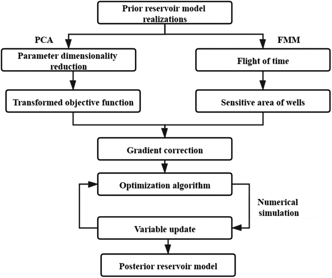
Figure 1: Calculation scheme of history matching

2  Methodology

2.1 FMM Method

The pressure wave diffusion equation (Eq. (1)) was derived by using the asymptotic ray theory of geometrical optics and seismology [31].

∇⋅(kμ∇→p)=φCt∂p∂t (1)

where, k is permeability, μ is fluid viscosity, P is pressure, φ is porosity, Ct is the comprehensive compressibility coefficient, t is the time variable. Fourier transform and asymptotic expansion of Eq. (1) can prove that under the high frequency limit, and the propagation of pressure wave front can be described by the Eikonal equation (Eq. (2)) [28–31]:

n(x→)|∇T(x→)|=1 (2)

where, T is the diffusion flight time at the x position; n=βk/(μφCt) is the diffusion factor; β is the unit conversion factor with a constant value of 0.0853. FMM tracks the leading edge of pressure wave by solving the Eikonal equation. Herein, upwind difference method is introduced to solve Eq. (2):

max(T−TxΔx/vx,0)2+max(T−TyΔy/vy,0)2+max(T−TzΔz/vz,0)2=1 (3)

where,

Tx=min(Ti−1,j,k,Ti+1,j,k)

Ty=min(Ti,j−1,k,Ti,j+1,k)

Tz=min(Ti,j,k−1,Ti,j,k+1)

where, T is the flight time at position (i, j, k); Δx, Δy and Δz are the grid size on the x, y, z directions, respectively; vx, vy and vz are the propagation velocity in the x, y, z directions, respectively; Tx, Ty and Tz are the grid tracking time in the x, y, z directions, respectively. As shown in Fig. 2, by considering reservoir permeability anisotropy in Cartesian grid system, the process to track the flight time is as following:

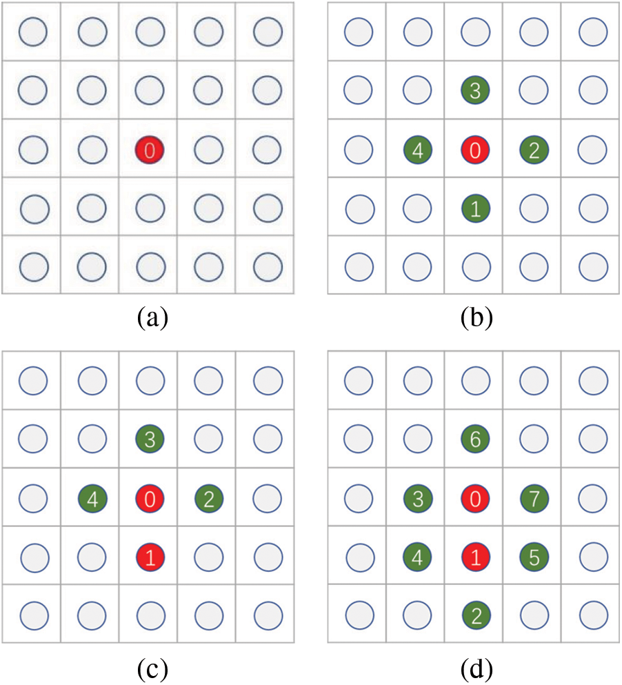
Figure 2: Flight time tracking process (a) Step 1 (b) Step 2 (c) Step 3 (d) Step 4

(1) Set the initial start grid and then mark it as a freezing grid (red point in Fig. 1a);

(2) Search for adjacent grids and calculate the flight time T;

(3) Find the grid to which the minimum flight time is required (“1” point in Fig. 1b and mark it as new freezing grid);

(4) Search for adjacent grids surround the freezing grid. Then calculate the flight time and set a new freezing grid (“2” point in Fig. 1d);

(5) Repeat Steps 2 to 4 until all grids are marked as freezing grids.

In order to reduce the calculation cost, we set the time threshold of single-well sensitive area to a preliminarily defined tracking range. In this paper, we arranged 1/T it from large to small and calculated the cumulative value. When the cumulative value accounted for 99% of the sum, all the grids with values less than the time threshold are set as the initial tracking range of the well.

2.2 Principle of History Matching

In this section, we first briefly described the mathematical model of history matching and the process to do parameter dimensionality reduction. Then, we explained how to use the single-well sensitive area data to correct the gradient of the objective function.

2.2.1 Mathematical Model of History Matching

History matching is a typical inverse-problem solving process, which aims to generate the maximum posteriori estimate of the reservoir model by matching the observation data. The correction between the actual observation data and the model parameters is:

dobs=g(m)+ed (4)

where, dobs is the observed data, such as water content, oil production rate, bottom hole pressure, etc.; g( ) refers to the numerical simulation process; m is the model parameter; ed is the measuring error. According to the Bayesian framework, the conditional PDF of m conditional dobs can be written as:

p(m|dobs)=p(dobs|m)p(m)p(dobs)∝p(dobs|m)p(m) (5)

where,

p(m|dobs)∝exp[−12(dobs−g(m))TCD−1(dobs−g(m))−12(m−mprior)TCM−1(m−mprior)] (6)

where, CM is the correlation matrix of model parameters; CD is the covariance matrix of measuring errors. Thus, in the history matching process, the following formula should be minimized:

f(m)=12(dobs−g(m))TCD−1(dobs−g(m))+12(m−mprior)TCM−1(m−mprior) (7)

where, mprior is the prior estimation vector of reservoir model. In the history matching process, the prior model was often used as the initial value of the continuous iteratives. Since mprior often follows the multivariate Gaussian distribution in practical applications, the average values of these prior model parameter that represented the prior geological features would be optimized as the initial value. In this paper, m¯ is used instead of mprior:

m¯=1Nr∑i=1Nrmj≈mprior (8)

In general, the actual reservoir parameters often have high dimensionality, making it pretty difficult to directly calculate the CM. In the past, many methods such as K-L decomposition method, discrete cosine transform method and gradual deformation method have been applied to reduce the dimensionality of the parameters in history matching. In this paper, efficient SVD decomposition method in PCA was introduced to parameterize the reservoir model and to deconstruct the CM to make Nw non-zero singular values. CM was calculated as following:

CM≈1Nr−1UwΛw2UwT (9)

where, Λw is the diagonal matrix, in which diagonal elements are singular values; Uw is the singular matrix. Herein, we defined a vector w, and m could be expressed by w:

w=Nr−1Λw−TUwT(m−m¯) (10)

The objective function can be approximately converted to:

f(w)=12(dobs−g(w))TCD−1(dobs−g(w))+12wTw (11)

The maximum posteriori estimation mMAP could be inversely calculated after the maximum posteriori estimation wMAP was obtained by minimizing Eq. (11):

mMAP=m¯+AwMAP (12)

where, A=UwΛwNr−1 .

2.2.2 Correction Method to Correct Gradients

In the numerical simulation process, the production data generated by the reservoir model based on the model parameters m generally followed the following relationship:

g(m)=Gm (13)

where, g(m) is the simulated data; G is the sensitivity matrix of g(m). The gradient of Eq. (11) can be written as

∇f(w)=w+GwTCD−1(g(w)−dobs) (14)

where, Gw is the sensitivity coefficient matrix of g(w). At the l iteration step, the variable could be updated by:

wl+1=wl−αl(wl+GwTCD−1(g(w)−dobs)) (15)

where, αl is the step size in search. In the previous study, the sensitivity matrix G was constructed over the m field. After parameterization, it was necessary to transfer the sensitivity matrix over m field to over w field, that was, transferring G to Gw. Herein, we defined ρ(m) as the sensitivity localization function over the m-field: ρ(m)=[ρ1,ρ2,...ρNd] . The gradient of ρ(m) is:

∂ρ∂m=(∂ρ1∂m1∂ρNd∂m1⋮⋱∂ρj∂mi⋱⋮∂ρ1∂mNm⋯∂ρNd∂mNm)(j=1,...Ndi=1,...Nm) (16)

where, Nd is the number of the observation data. After the single-well sensitive area was obtained by FMM, the sensitivity gradient beyond the sensitivity area was defined as ∂ρ∂m=0 . Based on the flight time, a exponential model was used to obtain the single-well sensitivity localization correlation model inside the sensitivity area:

∂ρ∂m={exp[−3T(m)/Tref(m)]⁡⁡⁡T∈Fj0⁡⁡⁡⁡⁡⁡⁡⁡⁡⁡⁡⁡⁡⁡⁡T∉Fj (17)

where, Fj is the sensitive area of well j generated by FMM; Tref is the maximum flight time within the sensitive area of well j, which is related to the static parameter field m. It was also worth noting that the flight time could be normalized to make the localization model more applicable.

Then we defined ρ(w) as the sensitivity localization function over the w field. Set:

∇w(ρ(w))=∂ρ∂w (18)

and

∇m(ρ(m))=∂ρ∂m. (19)

According to the chain rule to solve the partial derivatives:

∇w(ρ(w))=∇w(mT(w))∇m(ρ(m)) (20)

where, ∇w(mT(w))=AT . Therefore, localized analytical gradient considering the single-well sensitive area could be obtained by the Schur product between ∂ρ∂w and GwT . The latest updated variables were:

wl+1=wl−αl(wl+(∂ρ∂w◯GwT)CD−1(g(w)−dobs)) (21)

3  Case Study

3.1 Conceptual Case

A two-dimensional heterogeneous reservoir model with three reservoir fluids, oil, gas and water was first constructed to verify the proposed method. The size of this model was set to be 20 × 30 × 1. The grid size is, Dx = Dy = 80 m, and Dz = 30 m. We selected twenty prior reservoir realizations and a real model that provided the observation data. The real permeability field of the model was shown in Fig. 4a, which was of strong heterogeneity with high permeability zones. Fig. 4b was the average permeability field of twenty reservoir models. The average model was to be used as the initial model for history matching. Fig. 4c was the permeability field of a specific model. For all of models, the average porosity was 0.2, the initial water saturation was 0.2, and the gas was dissolved gas. More fluid physical properties could be seen in Table 1 and Fig. 3. There were one injection well and five production wells. The injection rate was a constant of 500 m3/d. The liquid flow rate of the production wells, 100 m3/d. A total of 1200 parameters including permeability and porosity were to be estimated by matching the actual production data.

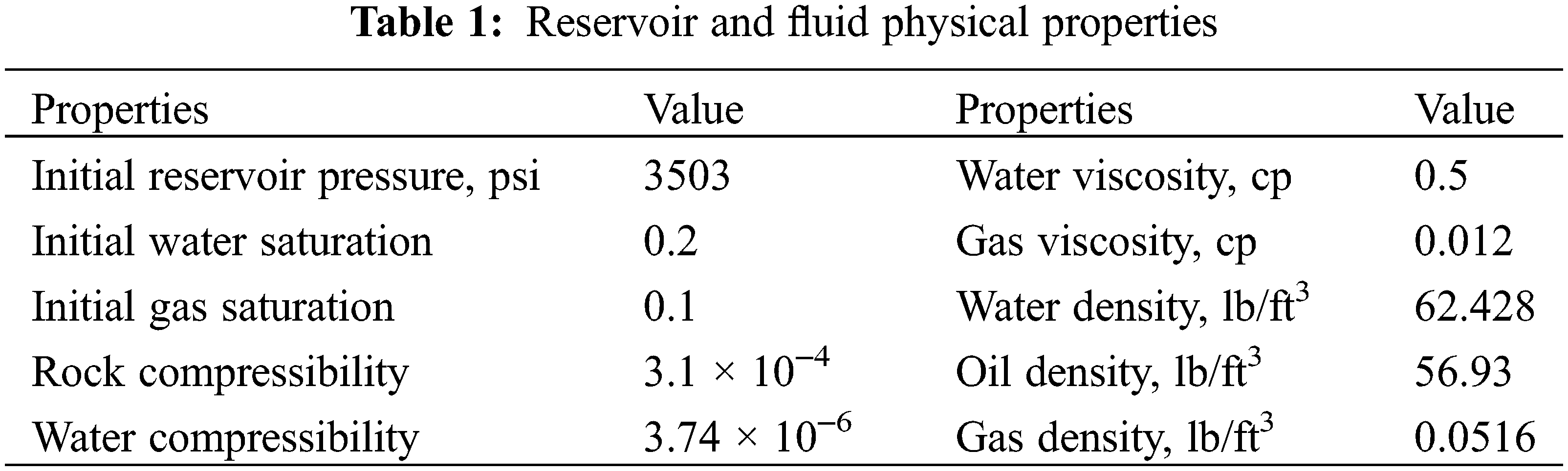
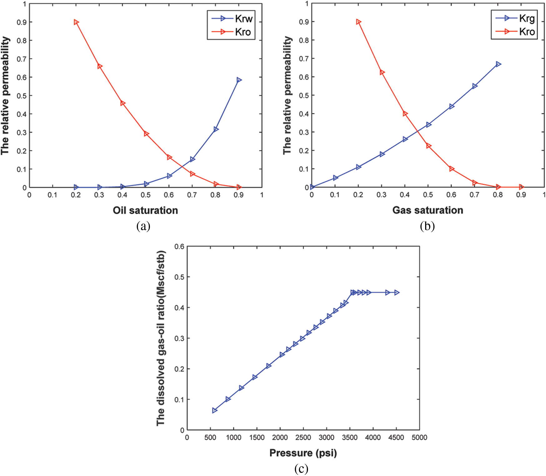
Figure 3: Fluid physical properties (a) oil-water relative permeability (b) oil-gas relative permeability (c) the dissolved gas-oil ratio vs. pressure

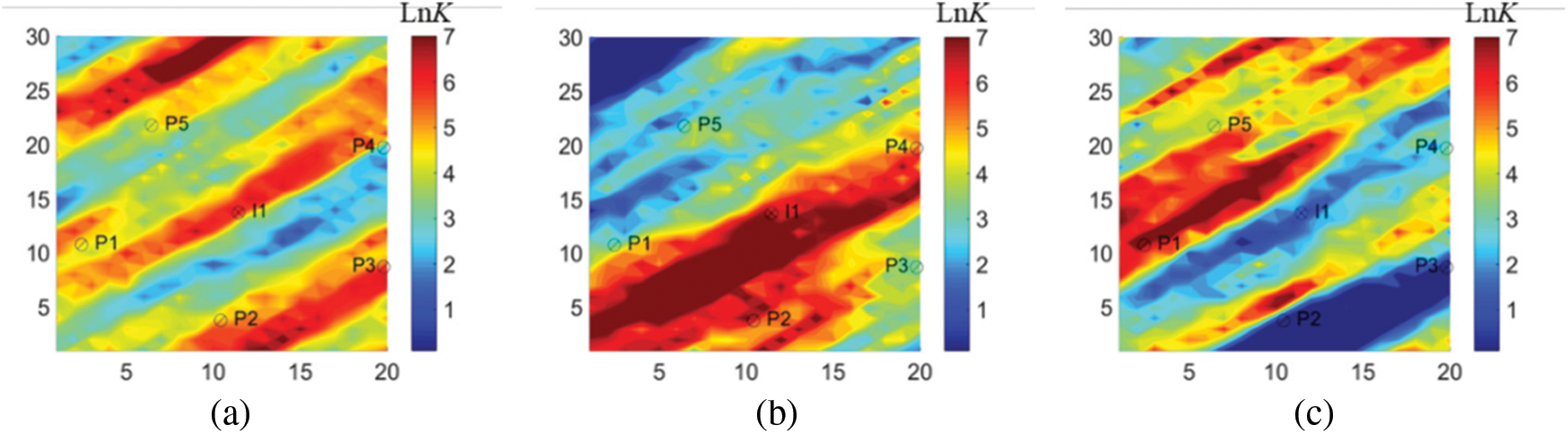
Figure 4: Log-permeability field (a) true model (b) average model (c) a specific model

In the history matching process, the FMM method was firstly used to calculate the flight time. Taking the injection well in the average model as an example (Fig. 5), the flight time was found to be related to permeability field. According to Eq. (1), the calculated migration velocity of the pressure wave was also related to the reservoir permeability. Generally speaking, higher permeability corresponds to better reservoir physical properties, and the flight time would be shorter. Based on the flight time, the sensitive area of each single well was then determined to localize the reservoir, as shown in Fig. 6. It was also worth mentioning that it only took 1.3 s to calculate the flight time without any numerical simulation runs, indicating the higher efficiency of FMM for sensitive area division as compared to the traditional methods based on experience, seismic data [32] or Voronoi diagram [33].

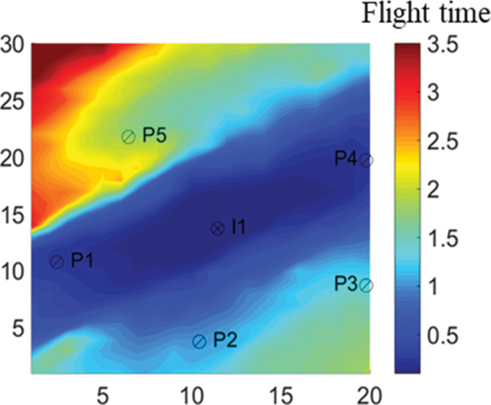
Figure 5: The flight time

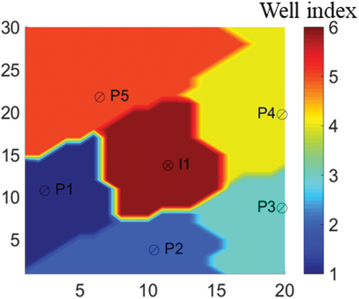
Figure 6: Single-well sensitive area

Subsequently, the PCA method was used to reduce the dimensionality of the parameters included in the reservoir model. In order to verify the effectiveness of the proposed method to weaken the pseudo-correlation, the finite difference method (FDM), simultaneous perturbation stochastic approximation (SPSA) [34,35], localized analytic gradient method (LAGM) and analytical gradient method without considering sensitive area (AGM) were adopted respectively to estimate the gradient of the objective function and to perform the history matching with 70 iterations. AGM refers to that the variable is updated by Eq. (15), and LAGM refers to that the variable is updated by Eq. (21). Some details about SPSA algorithm were listed in the Appendix A. For the four algorithms, the iteration step was set to 0.5. Figs. 7 and 8 were the calculated gradient by the four algorithms and its gradient correlation coefficient of each variable at the 10th and the 70th iteration step. Among them, the gradient calculated by FDM marked by red circles was considered as the true gradient. It was easy to notice that the LAGM gave a closer correlation with the true gradient than AGM and SPSA. For the calculated gradient correlation between FDM and the other three algorithms at the 10th iteration step, the SPSA marked by yellow line was 0.095, the AGM marked by gray line was 0.181, and the LAGM marked by blue line was 0.417. Similarly, at the 70th iteration step, the SPSA algorithm was 0.064, the AGM was 0.105, and the LAGM was 0.325. The results implied that the LAGM could effectively eliminate the pseudo correlation of the gradient. Fig. 9 was the convergence performance of the three algorithms within 70 iterations. In this example, LAGM and AGM yielded a final objective function value of about 7187. But LAGM showed a faster convergence speed, implying that LAGM had a higher computational efficiency for history matching process. The value of the final objective function obtained by SPSA was about 16601. Because SPSA required to perturb the variables synchronously for many times to obtain the approximate gradient, it often converged locally and required a higher computational cost. Also, it was tough to directly calculate the true gradient in history matching due to the huge numbers of reservoir parameters. Thus, parameterizing reservoir model and then modifying gradient might be a good choice for heavy reservoir history matching problem.

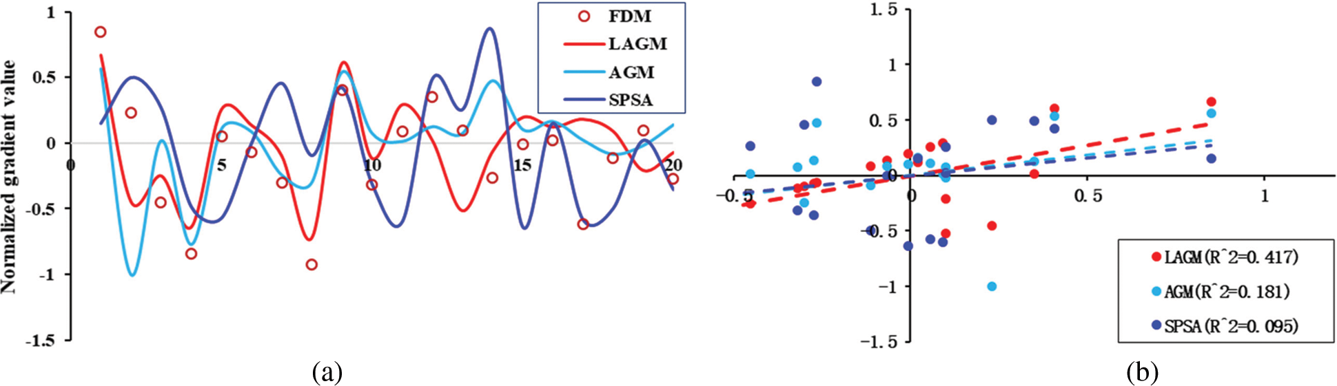
Figure 7: Calculated gradient information at 10th iteration step (a) Calculated normalized gradient for four algorithms (b) Gradient correlation coefficient between FDM and LAGM, AGM and SPSA

Figure 8: Calculated gradient information at 70th iteration step (a) Calculated normalized gradient for four algorithms (b) Gradient correlation coefficient between FDM and LAGM, AGM and SPSA

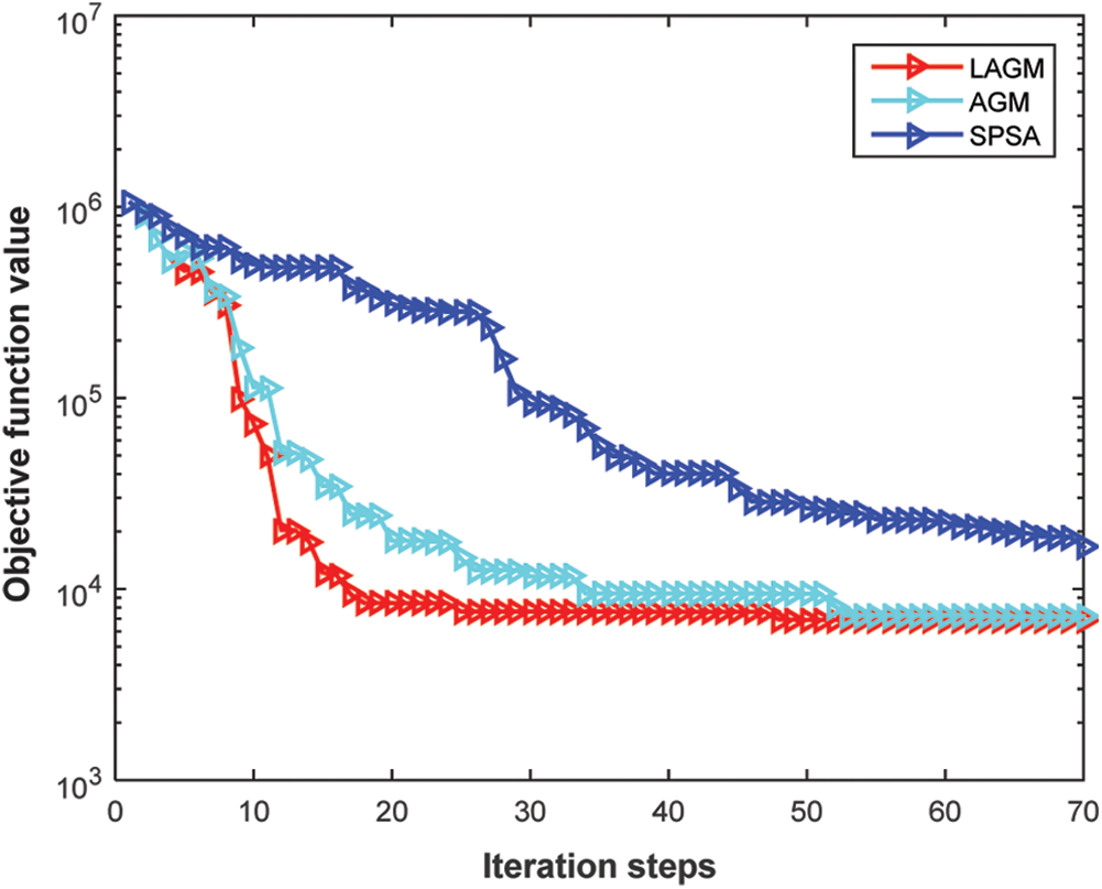
Figure 9: Objective function vs. the iteration steps

The final permeability estimates calculated by the three algorithms were presented in Fig. 10. The true model was obtained by FDM. By visual comparations, LAGM could reflect heterogeneous characteristics more accurate than AGM. In contrast, the permeability field obtained by SPSA gave more prominent heterogeneous characteristics. However, the obtained permeability field generated by SPSA was totally different as the true model in the upper left corner and lower right corner. The production predictions by the three algorithms were provided in Fig. 11. In this figure, the predictions of the initial model m¯ were marked by grey line. The observation data simulated by the true model was marked by the red circle. LAGM gave better history matching quality than the other two algorithms. However, for P3 well, no algorithms produced good results. Table 2 also showed that LAGM had higher calculation accuracy than the other two algorithms. This case mainly proved that the proposed method could effectively weaken the pseudo correlation and further improve the quality of history matching by using the single-well sensitive area and modified gradient.

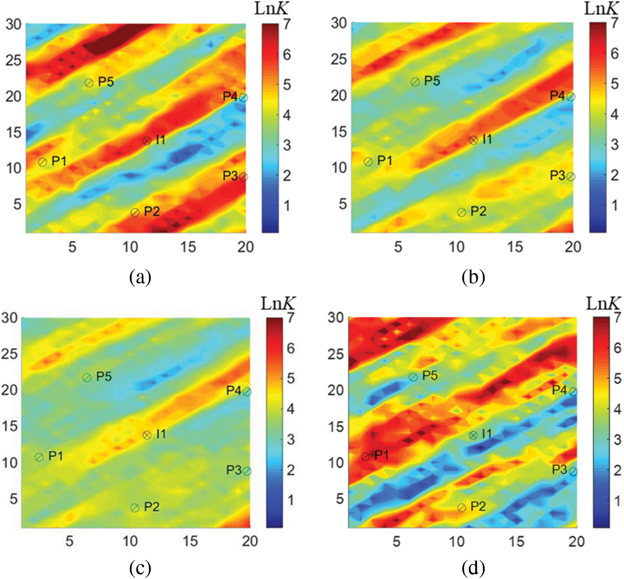
Figure 10: Log-permeability field of the history-matched model based on four algorithms (a) true model (b) LAGM (c) AGM (d) SPSA

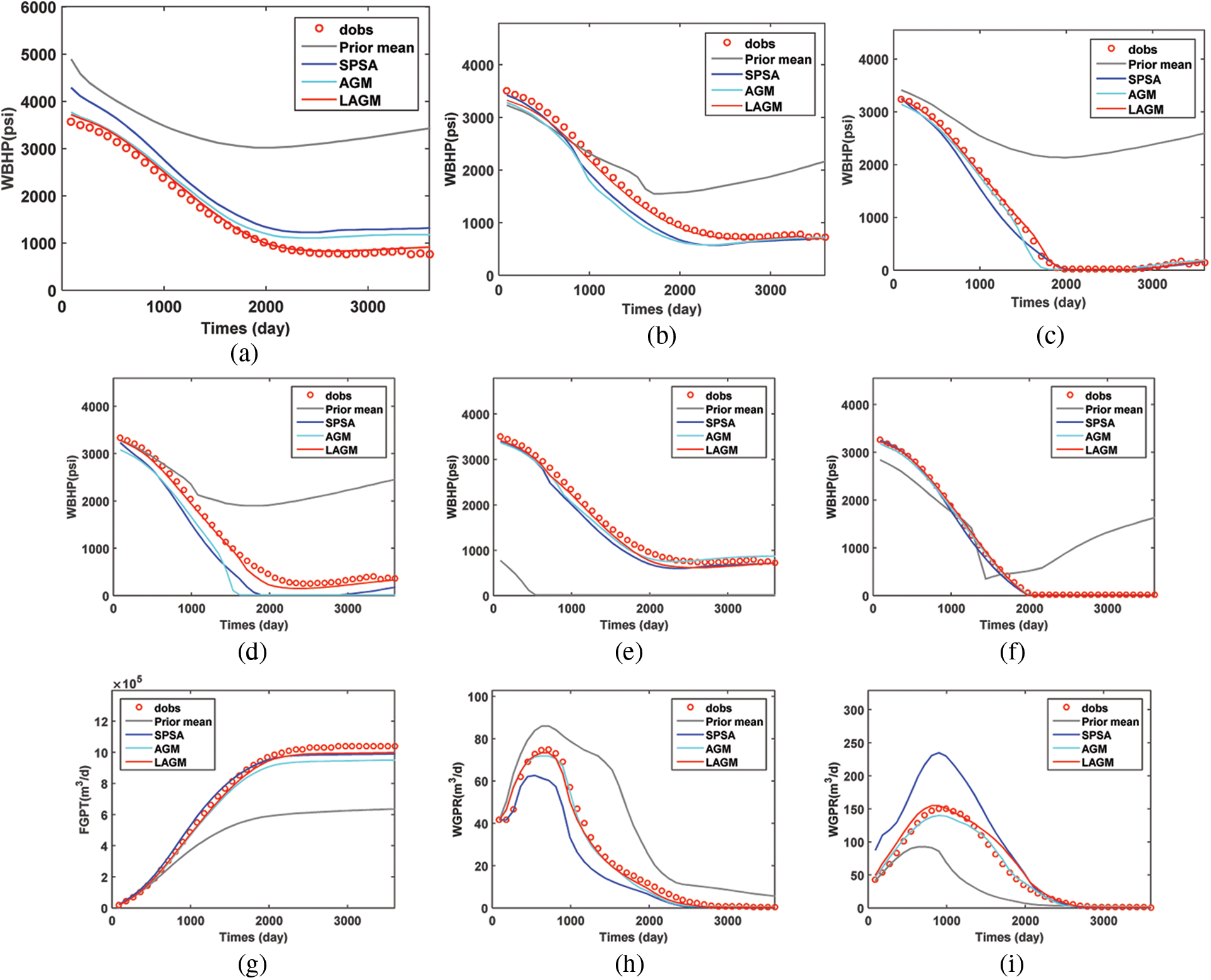
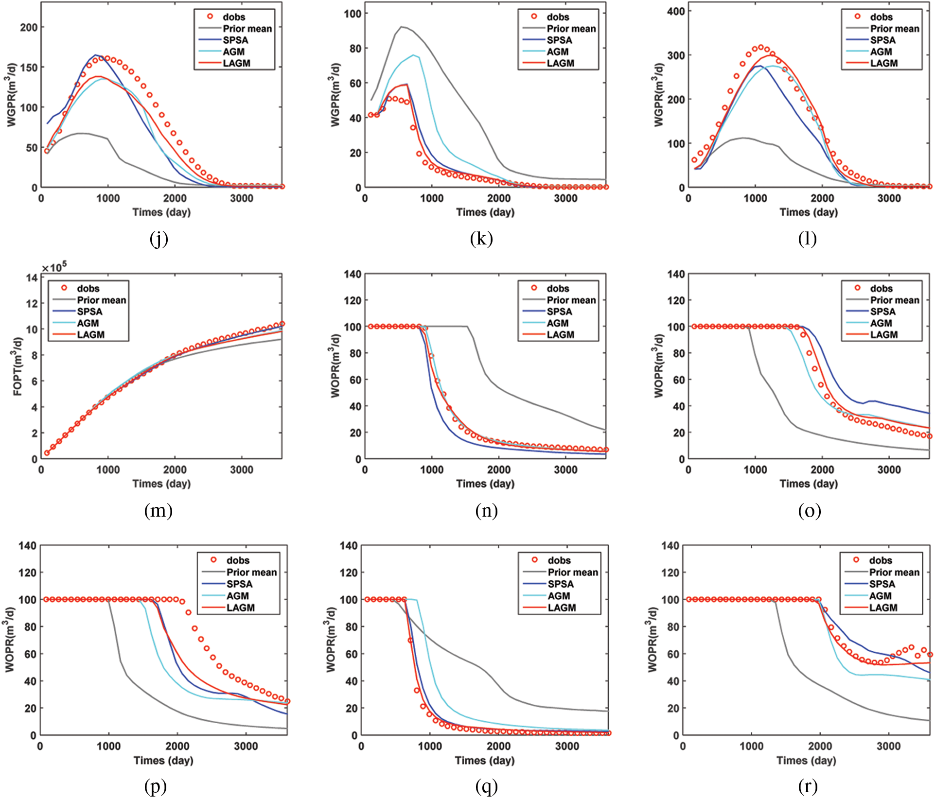
Figure 11: Production predictions of the history-matched model (a) I1 BHP (b) P1 BHP (c) P2 BHP (d) P3 BHP (e) P4 BHP (f) P5 BHP (g) FGPT (h) P1 WGPR (i) P2 WGPR (j) P3 WGPR (k) P4 WGPR (l) P5 WGPR (m) FOPT (n) P1 WOPR (o) P2 WOPR (p) P3 WOPR (q) P4 WOPR (r) P5 WOPR

3.2 Field Case

The Brugge oilfield was developed by TNO as a benchmark for closed-loop reservoir management test. Fig. 12 was the top structure of this reservoir. The grid represents the reservoir was divided into 139 × 48 × 9 grids, and the number of active grids is 44550. There are 20 production wells in the center and 10 injection wells at the edge to replenish energy within a lifetime of 7300 days. The injection rate was set to be 4000 m3/day and the production rate was 600 m3/day. In the history matching process, the variance of the measuring error was a fixed value of 0.05 over the observation data. The grid planar permeability was set to be the estimated parameter. Similar to the previously discussed example, 40 reservoir parameters were applied. Fig. 14a was the log-permeability field of the average model.

Then, FMM was introduced to calculate the flight time and to determine the single-well sensitive area. The sensitivity area of the first layer of the average model was shown in Fig. 13. The calculated flight time between grids with very long spatial distance was small due to the influence of strongly heterogeneous grids, resulting in noises. Therefore, we artificially eliminated some small noise in each area to improve the quality of history matching. Fig. 14 was the posterior estimate of permeability parameters generated by LAGM, AGM and SPSA algorithms at the 300th iteration step. LAGM and AGM gave very similar results in the MAP estimates, while SPSA gave more prominent heterogeneous characteristics. Fig. 15 was the matched production data of six wells. The production performances simulated by the average model diverted from the observations. LAGM algorithm showed better prediction results compared to other two algorithms. Table 3 presented the calculation accuracy of the three algorithms, indicating that LAGM had higher calculation accuracy in applications.

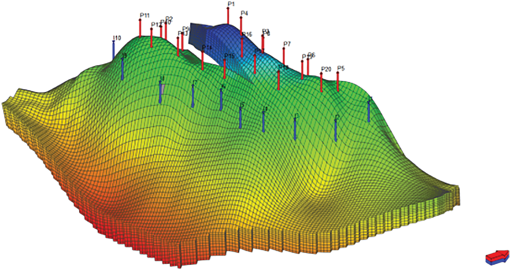
Figure 12: Reservoir structure

Figure 13: Single-well sensitive area

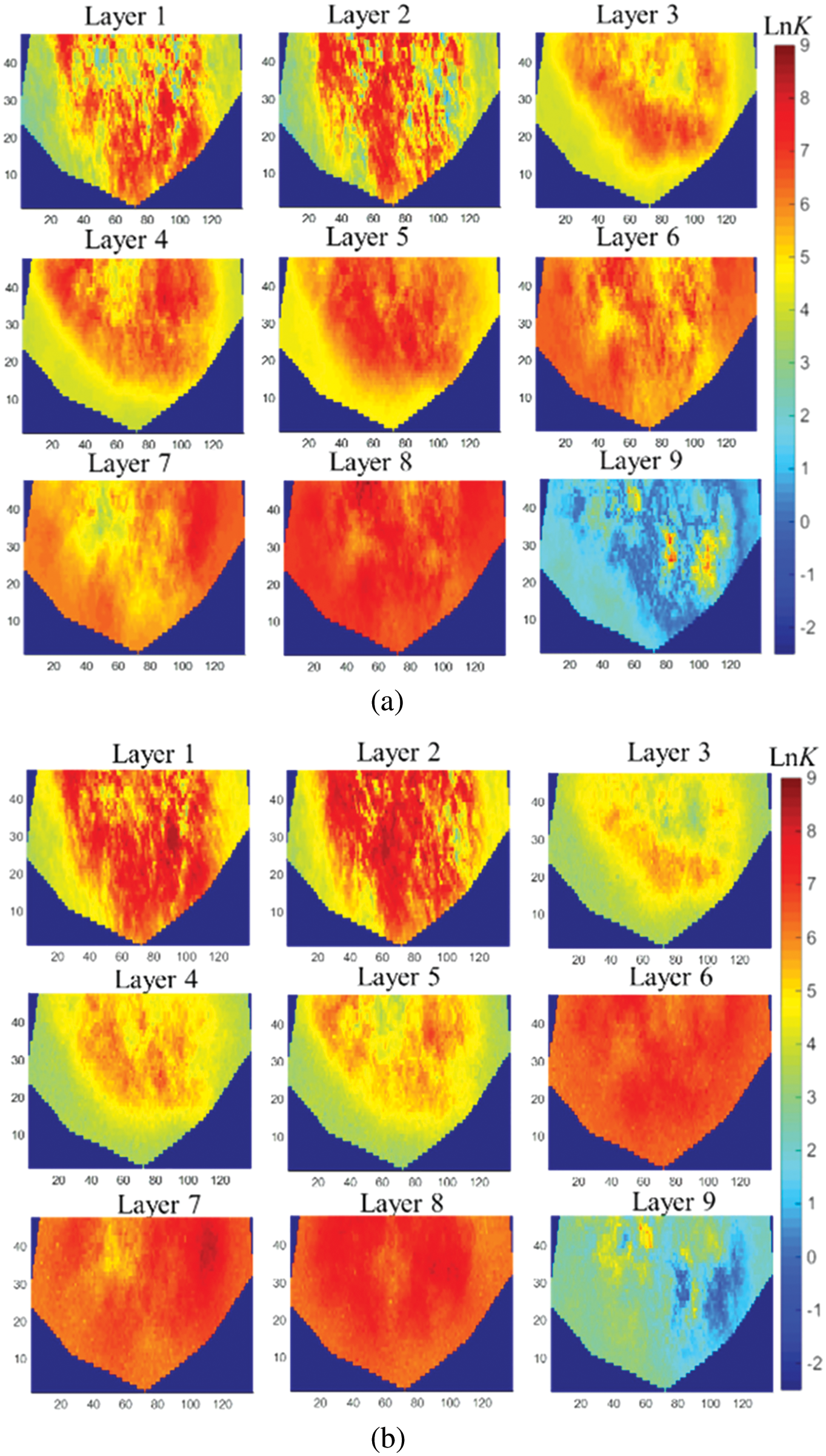
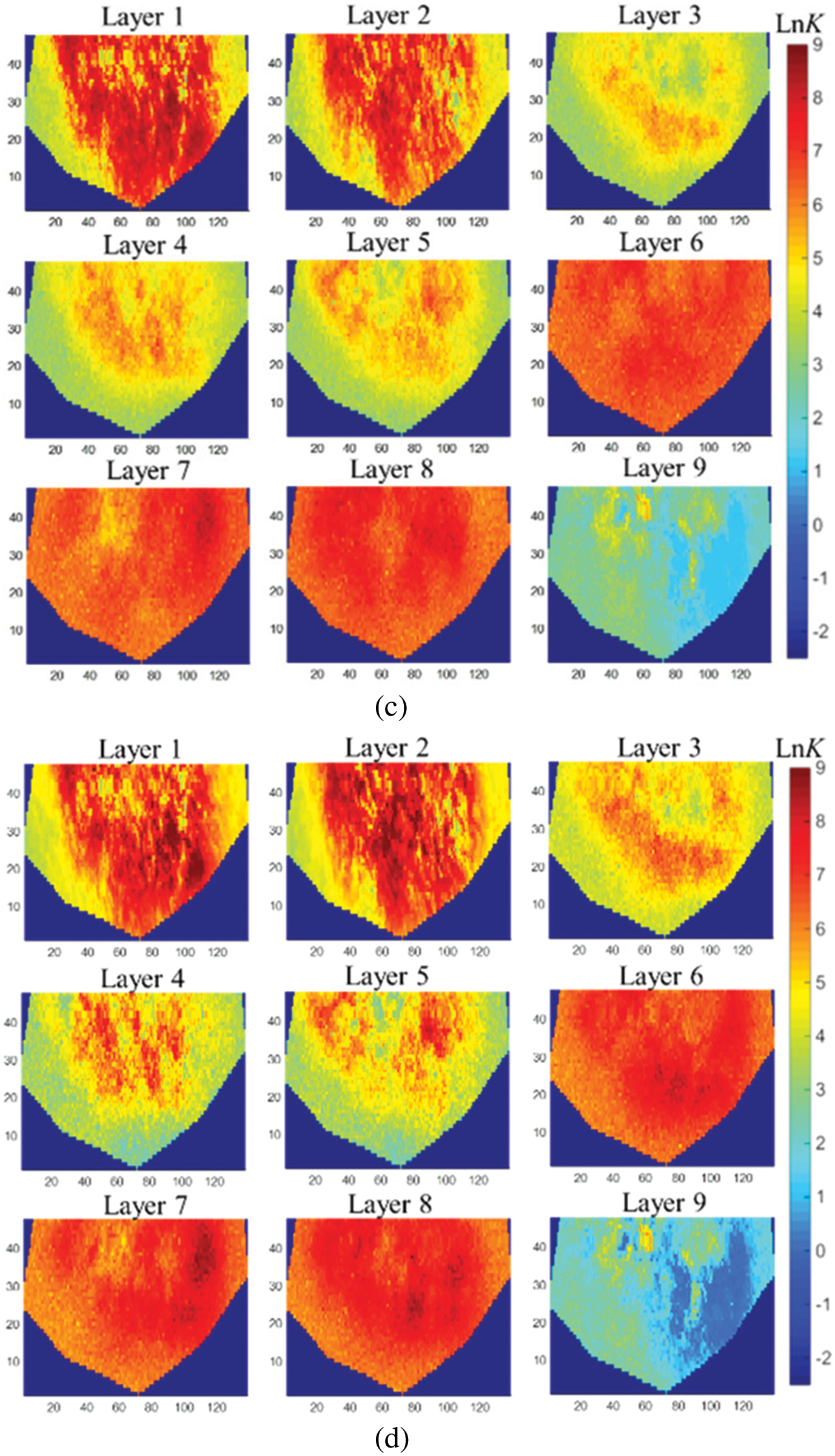
Figure 14: Log-permeability field of history-matched models (a) average model (b) LAGM (c) AGM (d) SPSA

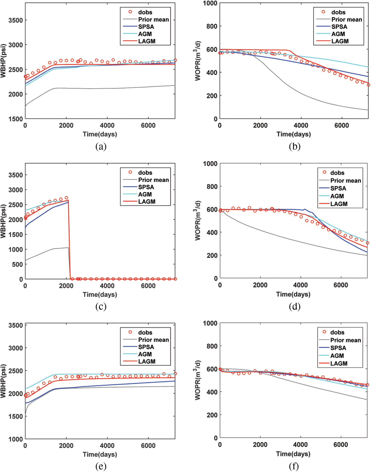
Figure 15: Production predictions of the history-matched model (a) I1 WBHP (b) P3 (c) I2 WBHP (d) P5 (e) P12 WBHP (f) P14

4  Conclusion

In this paper, we firstly reviewed the theorem of FMM and briefly introduced the sensitive area division method. Subsequently, we established a history matching mathematical model based on Bayesian framework. A parameterization method was used to reduce the dimensionality of original model parameters. By integrating the sensitive area information, the gradient of history matching could be better modified. The proposed approach was actually a two-step history matching method and no numerical simulation runs were required in the pretreatment process. To evaluate the feasibility of the presented method, a conceptual case of water drive in a heterogeneous two-dimensional reservoir and a real field case were tested. The results showed that the presented approach had higher accuracy and computational efficiency as compared to non-localized gradient method and gradient free algorithm. Moreover, the presented idea could also be used in other history matching algorithms, such as ENKF, ES-MDA, and so on. It was worth noting that parameterizing reservoir model and then modifying gradient may be a good choice for heavy reservoir history matching problem.

Funding Statement: This study was supported by National Natural Science Foundation of China (Nos. 52104017, 51874044, 51922007), Southern Marine Science and Engineering Guangdong Laboratory (Zhanjiang) (No. zjw-2019-04).

Conflicts of Interest: The authors declare that they have no conflicts of interest to report regarding the present study.

References

 1.  Afshari, S., Aminshahidy, B., Pishvaie, M. R. (2011). Application of an improved harmony search algorithm in well placement optimization using streamline simulation. Journal of Petroleum Science and Engineering, 78(3–4), 664–678. DOI 10.1016/j.petrol.2011.08.009. [Google Scholar] [CrossRef]

 2.  Amirsardari, M., Dabir, B., Naderifar, A. (2016). Development of a flow based dynamic gridding approach for fluid flow modeling in heterogeneous reservoirs. Journal of Natural Gas Science and Engineering, 31, 715–729. DOI 10.1016/j.jngse.2016.03.077. [Google Scholar] [CrossRef]

 3.  Bertolini, A. C., Maschio, C., Schiozer, D. J. (2015). A methodology to evaluate and reduce reservoir uncertainties using multivariate distribution. Journal of Petroleum Science and Engineering, 128(1), 1–14. DOI 10.1016/j.petrol.2015.02.003. [Google Scholar] [CrossRef]

 4.  Suri, Y., Islam, S. Z., Stephen, K., Donald, C., Thompson, M. et al. (2020). Numerical fluid flow modelling in multiple fractured porous reservoirs. Fluid Dynamics & Materials Processing, 16(2), 245–266. DOI 10.32604/fdmp.2020.06505. [Google Scholar] [CrossRef]

 5.  Ma, L., He, L., Luo, X., Mi, X. (2021). Numerical simulation and experimental analysis of the influence of asymmetric pressure conditions on the splitting of a gas-liquid two-phase flow at a T-Junction. Fluid Dynamics & Materials Processing, 17(5), 959–970. DOI 10.32604/fdmp.2021.016710. [Google Scholar] [CrossRef]

 6.  Yang, P. H., Watson, A. T. (1988). Automatic history matching with variable-metric methods. SPE Reservoir Engineering, 3(3), 995–1001. DOI 10.2118/16977-PA. [Google Scholar] [CrossRef]

 7.  Zhang, F., Reynolds, A. C. (2002). Optimization algorithms for automatic history matching of production data. Proceedings of the European Conference on the Mathematics of Oil Recovery. [Google Scholar]

 8.  Emerick, A. A., Reynolds, A. C. (2010). EnKF-MCMC. SPE EUROPEC/EAGE Annual Conference and Exhibition. SPE 131375-MS. [Google Scholar]

 9.  Emerick, A. A., Reynolds, A. C. (2013). Ensemble smoother with multiple data assimilation. Computers & Geosciences, 55(3), 3–15. DOI 10.1016/j.cageo.2012.03.011. [Google Scholar] [CrossRef]

10. Gao, G., Li, G., Reynolds, A. C. (2007). A stochastic optimization algorithm for automatic history matching. SPE Journal, 12(2), 196–208. DOI 10.2118/90065-PA. [Google Scholar] [CrossRef]

11. Powell, M. J. (2006). The NEWUOA software for unconstrained optimization without derivatives in large-scale nonlinear optimization, pp. 255–297. Springer US: Large-Scale Nonlinear Optimization. [Google Scholar]

12. Marcelo, M., Jorge, N. (2001). Wedge trust region methods for derivative free optimization. Mathematical Programming, 91(2), 289–305. DOI 10.1007/s101070100264. [Google Scholar] [CrossRef]

13. Eberhart, R., Kennedy, J. (1995). A new optimizer using particle swarm theory. Proceedings of the Sixth International Symposium on Micro Machine and Human Science. [Google Scholar]

14. Romero, C. E., Carter, J. N., Gringarten, A. C. (2000). A modified genetic algorithm for reservoir characterization. International Oil and Gas Conference and Exhibition, SPE 64765-MS. [Google Scholar]

15. Hong, Y., Lu, L., Abousleiman, Y., Wang, H., Li, X. et al. (2018). High permeability zone prediction based on seismic multi-attributes analysis with PCA fusion in IRAQ Ahdeb Oilfield. 2018 SEG International Exposition and Annual Meeting. [Google Scholar]

16. Wilson, A. (2015). Integrating PCA and streamline information for history matching channelized reservoirs. Journal of Petroleum Technology, 67(4), 138–141. DOI 10.2118/0415-0138-JPT. [Google Scholar] [CrossRef]

17. Tavakoli, R., Reynolds, A. C. (2009). History matching with parameterization based on the singular value decomposition of a dimensionless sensitivity matrix. SPE Journal, 15(2), 495–508. DOI 10.2118/118952-PA. [Google Scholar] [CrossRef]

18. Sarma, P., Durlofsky, L. J., Aziz, K., Chen, W. H. (2007). A new approach to automatic history matching using kernel PCA. SPE Reservoir Simulation Symposium, Houston. SPE-106176-MS. [Google Scholar]

19. Gharbi, R. B., Smaoui, N., Peters, E. J. (1998). Unstable EOR displacements and their prediction using the Karhunen-Loeve (K-L) decomposition. The International Petroleum Conference and Exhibition of Mexico. [Google Scholar]

20. Yang, X., Zhu, P. (2017). Stochastic seismic inversion of nonstationary model based on multigrid gradual deformation method. The 2017 SEG International Exposition and Annual Meeting. [Google Scholar]

21. RamaRao, B. S., LaVenue, A. M. (1995). Pilot point methodology for automated calibration of an ensemble of conditionally simulated transmissivity fields: 1. Theory and computational experiments. Water Resources Research, 31(3), 475–493. DOI 10.1029/94WR02258. [Google Scholar] [CrossRef]

22. Kim, S., Kim, J., Jung, H., Lee, C., Lee, K. et al. (2016). Characterization of 3D channelized gas reservoirs with an aquifer using EnKF, DCT, and PFR. 26th International Ocean and Polar Engineering Conference. [Google Scholar]

23. Xie, J., Mondal, A., Efendiev, Y., Mallick, B., Akhil, D. (2010). History matching channelized reservoirs using reversible jump markov chain monte carlo methods. SPE Improved Oil Recovery Symposium, pp. 393–412. [Google Scholar]

24. Han, J., Chen, R., Akhil, D. (2016). Multiscale method for history matching channelized reservoirs using level sets. Paper presented at the SPE Annual Technical Conference and Exhibition. SPE-181461-MS. [Google Scholar]

25. Han, Y., Zhao, H. (2013). TOT project financing risk assessment based on PCA. Proceedings of 2013 3rd International Conference on Applied Social Science, pp. 461–465. [Google Scholar]

26. Carobene, A., Campagner, A., Uccheddu, C., Banfi, G., Vidali, M. et al. (2021). The multicenter European Biological Variation Study (EuBIVASA new glance provided by the Principal Component Analysis (PCAa machine learning unsupervised algorithms, based on the basic metabolic panel linked measurands. Clinical Chemistry and Laboratory Medicine. DOI 10.1515/cclm-2021-0599. [Google Scholar] [CrossRef]

27. Liu, W., Zhao, H., Lei, Z. X., Chen, Z. S., Cao, L. et al. (2019). Reservoir assisted history matching method using a local ensemble Kalman filter based on single-well sensitivity region. Acta Petrolei Sinica, 40(6), 716–725. DOI 10.7623/syxb201906007. [Google Scholar] [CrossRef]

28. Sethian, J. A., Popovici, A. M. (1999). 3-D traveltime computation using the fast marching method. Geophysics, 64(2), 516–523. DOI 10.1190/1.1444558. [Google Scholar] [CrossRef]

29. Sethian, J. A. (2001). Implementation and application of level set and fast marching methods for advancing fronts. Journal of Computational Physics, 169(2), 503–555. DOI 10.1006/jcph.2000.6657. [Google Scholar] [CrossRef]

30. Rawlinson, N., Sambridge, M. (2018). The fast marching method: An effective tool for tomographic imaging and tracking multiple phases in complex layered media. Exploration Geophysics, 36(4), 341–350. DOI 10.1071/EG05341. [Google Scholar] [CrossRef]

31. Vasco, D. W., Keers, H., Karasaki, K. (2000). Estimation of reservoir properties using transient pressure data: An asymptotic approach, vol. 36, pp. 3447–3465. John Wiley & Sons, Ltd. [Google Scholar]

32. Roggero, F., Hu, L. Y. (1998). Gradual deformation of continuous geostatistical models for history matching. SPE Annual Technical Conference and Exhibition. SPE-49004. [Google Scholar]

33. Al-akhdar, S., Ding, D. Y., Dambrine, M., Jourdan, A. (2012). An integrated parameterization and optimization methodology for assisted history matching: Application to libyan field case. North Africa Technical Conference and Exhibition. SPE-150716-MS. [Google Scholar]

34. Spall, J. C. (1992). Multivariate stochastic approximation using a simultaneous perturbation gradient approximation. IEEE Transactions on Automatic Control, 37(3), 332–341. DOI 10.1109/9.119632. [Google Scholar] [CrossRef]

35. Spall, J. C. (2000). Adaptive stochastic approximation by the simultaneous perturbation method. IEEE Transactions on Automatic Control, 45(10), 1839–1853. DOI 10.1109/TAC.2000.880982. [Google Scholar] [CrossRef]

Appendix A: SPSA algorithm

As an approximate-gradient iterative optimization algorithm, SPSA can ensure that the optimization direction is always the uphill direction through the simultaneous disturbance of components of variable. For the lth iteration, the stochastic gradient of the target function in Eq. (11) can be calculated by

g^l(wl)=f(wl+clΔl)−f(wl−clΔl)2clΔl−1 (A-1)

where Δl is the random column vector that satisfies the +_1 Bernoulli distribution; cl is the positive coefficient controlling perturbation size with the fixed value of 0.101. The variable w is updated through steepest descent

w l+1 = w l + α l+1 g ^ ¯ l ( w l ) (A-2)

where αl+1 is the iteration step size with the fixed value of 0.5; the average gradient is defined by

g ^ ¯ l ( w l )= 1 p ∑ i=1 p g ^ l ( w l ) (A-3)

where p is the number of perturbation at each iteration with a fixed value of 5.

This work is licensed under a Creative Commons Attribution 4.0 International License, which permits unrestricted use, distribution, and reproduction in any medium, provided the original work is properly cited.