| Fluid Dynamics & Materials Processing |
DOI: 10.32604/fdmp.2022.019485
ARTICLE
Thermal Conductivity and Dynamic Viscosity of Highly Mineralized Water
1Building Engineering Educatation, Universitas Pendidikan Indonesia, Bandung, 45363, Indonesia
2Al-Nisour University College, Iraq, 10004, Baghdad
3Departamento de Energía, Universidad de la Costa, Barranquilla, 080002, Colombia
4Universitas Masoem, Bandung, 45363, Indonesia
5Department of Language, FPT University, Hanoi, 700000, Vietnam
6Kazan Federal University, Russia, Kazan, 420000, Russia
7Dentistry Department, Kut University College, Kut, Wasit, Iraq, College of Technical Engineering, The Islamic University, Najaf, 54001, Iraq
8National University of Science and Technology, Dhi-Qar, 64001, Iraq
9Department of Pharmacology, Saveetha Dental College and Hospital, Saveetha Institute of Medical and Technical Sciences, Chennai, 600056, India
*Corresponding Author: Dadang Mohamad. Email: m.mana.qeshm@gmail.com
Received: 26 September 2021; Accepted: 09 November 2021
Abstract: Further development in the field of geothermal energy require reliable reference data on the thermophysical properties of geothermal waters, namely, on the thermal conductivity and viscosity of aqueous salt solutions at temperatures of 293–473 K, pressures Ps = 100 MPa, and concentrations of 0–25 wt.%. Given the lack of data and models, especially for the dynamic viscosity of aqueous salt solutions at a pressure of above 40 MPa, generalized formulas are presented here, by which these gaps can be filled. The article presents a generalized formula for obtaining reliable data on the thermal conductivity of water aqueous solutions of salts for Ps = 100 MPa, temperatures of 293–473 K and concentrations of 0%–25% (wt.%), as well as generalized formulas for the dynamic viscosity of water up to pressures of 500 MPa and aqueous solutions of salts for Ps = 100 MPa, temperatures 333–473 K, and concentration 0%–25%. The obtained values agree with the experimental data within 1.6%.
Keywords: Thermal conductivity; dynamic viscosity; water-salt systems; aqueous solutions of salts; high pressure; multicomponent water-salt systems
For many years, solutions have attracted and continue to attract the attention of many researchers due to the important role they play in all natural phenomena of life and the complexity of their nature that is largely determined by the properties of the liquid phase in general. The development of power engineering and other industries is closely related to the use of a wide range of coolants and working fluids. Among the liquid heat carriers used in various sectors of the economy, aqueous and non-aqueous solutions of inorganic substances play an important role [1–6]. The use of suitable nano additives to improve and increase the cooling property in industrial devices can be effective in reducing the hot spot temperature, which is one of the design limitations [7,8]. It increases the nominal power, reduce the dimensions and consumables in equipment as coolant. Studies on nanofillers show that increasing the thermal conductivity of nanofluids depends on many variables [9–12]. These factors include nano-filler size, particle surface shape and area, filler volume, particle aggregation, stability, viscosity, brown motion and temperature effect. In this paper, these factors are introduced and how they affect the heat transfer of nanofluids. In one study, h-BN powder nanoparticles were used as fillers in ethylene glycol fluid [13]. After preparing nanofluids with filler values of 0.025 vol and 0.2% vol and examining their thermal conductivity, the results showed that the thermal conductivity for nanofluids with filler volume of 0.025% is higher than the other.
Aqueous solutions of electrolytes are widely used in power generation systems at thermal and nuclear power plants, plants using solar and geothermal energy, oil and gas industry. In such industries as the production of mineral fertilizers, electrochemical methods for the production of inorganic metal compounds by electrolysis of aqueous solutions, the production of soda, aqueous solutions of inorganic substances are widely used. For the effective use of aqueous solutions of electrolytes in these areas of technology, accurate information is required on their thermophysical properties, in particular, on thermal conductivity and dynamic viscosity in a wide range of state parameters. In modern technology, a variety of fluids are used as heat carriers. However, it is not always possible to timely obtain experimental data on the physical properties of these substances at high state parameters. This is especially true for thermal conductivity and dynamic viscosity, the experimental determination of which presents significant difficulties. Therefore, it is important to consider the equations that are the most reliable and convenient for calculation with sufficient approximation for practice [14,15].
Cooling fluids are used in many industrial fields such as electronics, refrigeration, air conditioning equipment and transportation. The thermal conductivity of these fluids plays a vital role in the development of high-performance heat transfer devices. Since solids have much higher thermal conductivity than conventional fluids, the idea of introducing heat-conducting particles into the fluid was considered. The thermophysical parameters measured include the thermal conductivity, thermal diffusivity, and specific heat capacity.
In this method the geothermal energy has developed on the thermophysical properties of geothermal waters, namely, on the thermal conductivity and viscosity of aqueous salt solutions at temperatures of 293–473 K, pressures Ps = 100 MPa, and concentrations of 0–25 wt.%. For this purpose a generalized formula for obtaining reliable data on the thermal conductivity of water in the pressure ranges Ps = 1000 MPa, temperatures of 293–473 K and the thermal conductivity of aqueous solutions of salts in the pressure ranges Ps = 100 MPa, temperatures of 293–473 K and concentrations of 0%–25% (wt.%), as well as generalized formulas for the dynamic viscosity of water up to pressures of 500 MPa and aqueous solutions of salts in the pressure ranges Ps = 100 MPa, temperatures 333–473 K, and concentration 0%–25%.
Maxwell was the first person who investigated thermal conductiv- ity, using particle suspension system. Maxwell’s model ignores the in- teractions between particles and the base fluid and assumes very low concentration of spherical particles. Other researchers have investigated the effects of different parame-ters such as particle morphology, surface energy, and heat resistance on thermal conductivity. Table 2 shows some of the current theoretical and empirical models used for nanoparticles. As can be seen, changes in thermal conductivity are dependent on volume fraction and temperature of nanofluids. high mineralized waters with purities of 99.9% and 99.5%, respectively, were used in the current study. An important challenge with nanofluids is that nanoparticles tend to accumulate due to molecular interactions such as van der Waals forces [16–21]. Therefore, as the percentage of filler increases, the accumulation of particles also increases. Also, the viscosity of the system increases and with decreasing the ratio of the effective surface area to the volume, the thermal performance of the fluid also decreases. In general, the accumulation velocity is determined by the collision frequency and the probability of cohesion during collision.
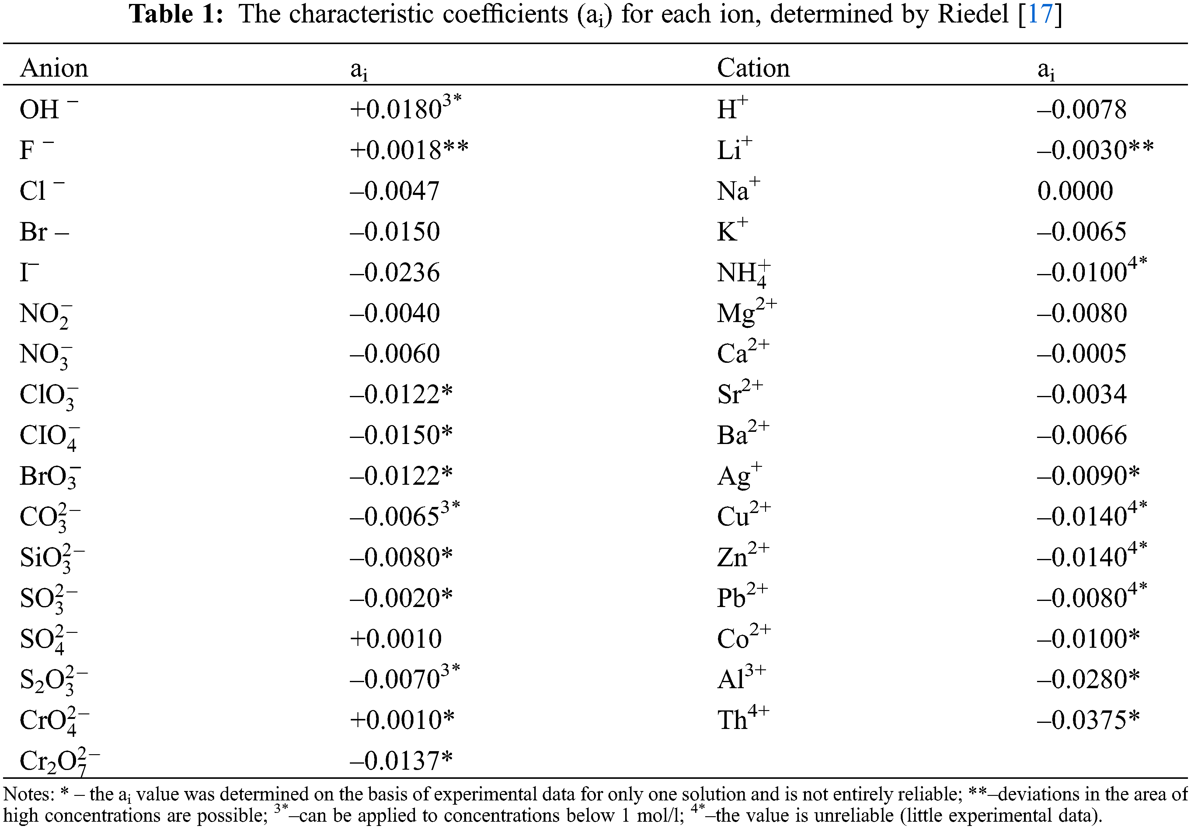
For aqueous solutions of binary and multicomponent inorganic substances, in [4,5] proposed a formula for determining the coefficient of thermal conductivity of aqueous solutions of salts, acids, and alkalis at a temperature of 293 K without the coefficient 1.163–for a unit of measurement of thermal conductivity in kcal/(m·h·deg), and the author of this paper introduced 1.163 to measure the thermal conductivity coefficient in W/(m·K):
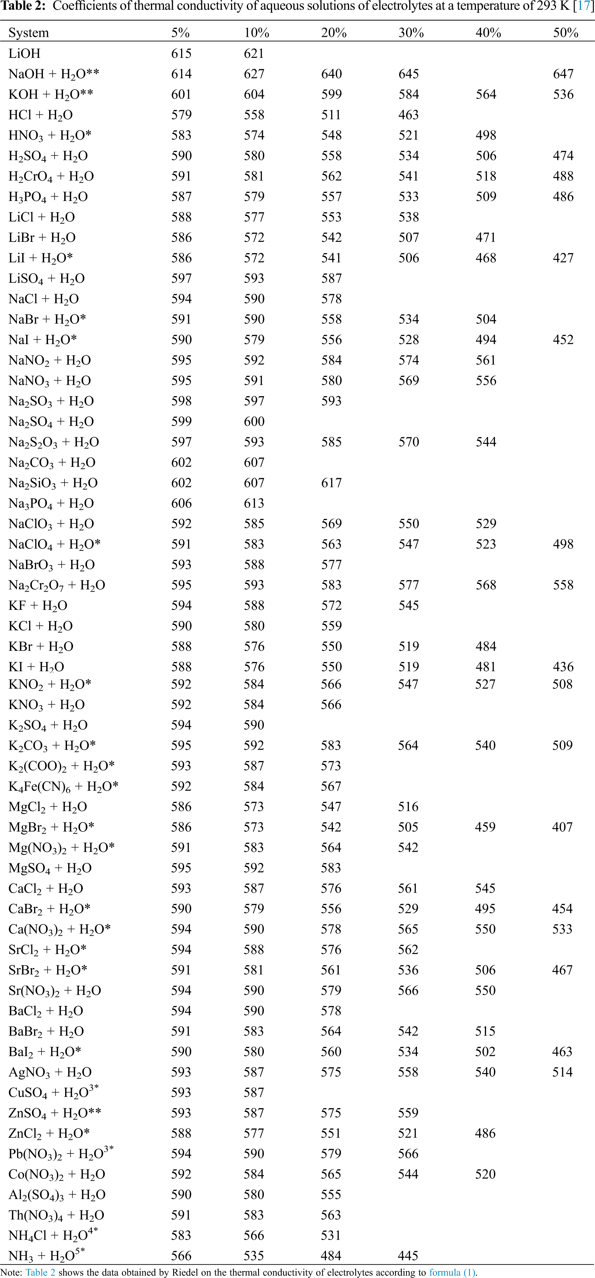
where 1.163–the coefficient of conversion of the unit of measurement of thermal conductivity from kcal/(m·h·deg) to W/(m·K). Typical coefficients (ai) are given in [4,5], and here they are presented in Table 1.
Note that N = 10 rc/m [3], where N is the concentration of the electrolyte, mol/dm3 of the solution; r– solution density, g/dm3; c–solution concentration, wt.%; m–the molar mass of the substance, g/mol. Data on the density of solutions of various water-salt systems and molar masses are given in [6], and ai – coefficients characteristic for each ion are presented in [4], and here in Table 2.
In formula (1), there is the letter N–the concentration of the electrolyte, mol/dm3 of the solution, which is needed in calculations when converting the concentration of the solution near the saturation line from mol/dm3 to % (wt). For this purpose, the author used the formula N =r10c/m and experimental and reference data [18].
In [19], it considered a formula for calculating the thermal conductivity of aqueous solutions of salts of acids and alkalis at temperatures of 293–373 K. The formula for the equality of the same ratios of the thermal conductivity of water and aqueous solutions at T = 273–373 K is the following:
The author’s studies have shown that formula (2) can be represented as (3) and (4) when using the values of thermal conductivity of water and aqueous solutions of electrolytes near the saturation line at temperatures of 293–473 K. If instead
Equation formulas for the ratio of thermal conductivity of water and aqueous solutions of electrolytes at temperatures of 273–473 K [5] are the following:
The deviation of the calculated values of the thermal conductivity of aqueous salt solutions near the saturation line according to formula (4) from the experimental data [4,5,9] was less than 1.3%, and from the data according to formula (1) at a temperature of 293 K, less than 1% (because formula (1) is only for one temperature–293 K).
The effect of salt on the thermal conductivity of the solution is manifested in the same way at all temperatures, when taking the interval of 293–473 K at pressures of 0.1–2 MPa.
In calculations by formula (4), critically estimated experimental values of the thermal conductivity of water in a state of saturation [22] were used, and the characteristic coefficients for each ion ai were those from [4] (given in Table 1) and new ones, which were obtained by the author using formula (4).
Note that ai for most aqueous solutions of salts, acids, and alkalis (anions and cations) consist of negative numbers.
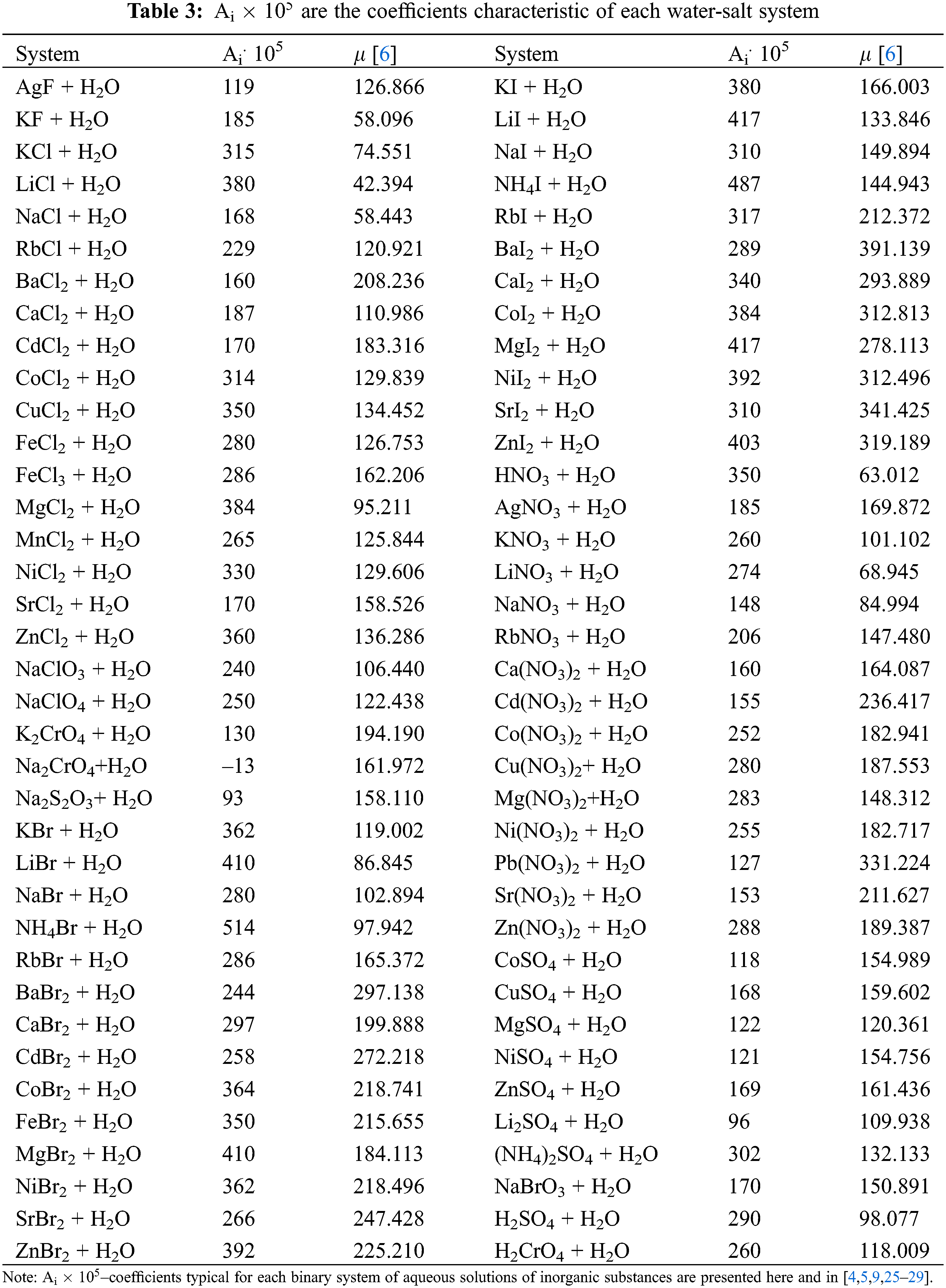
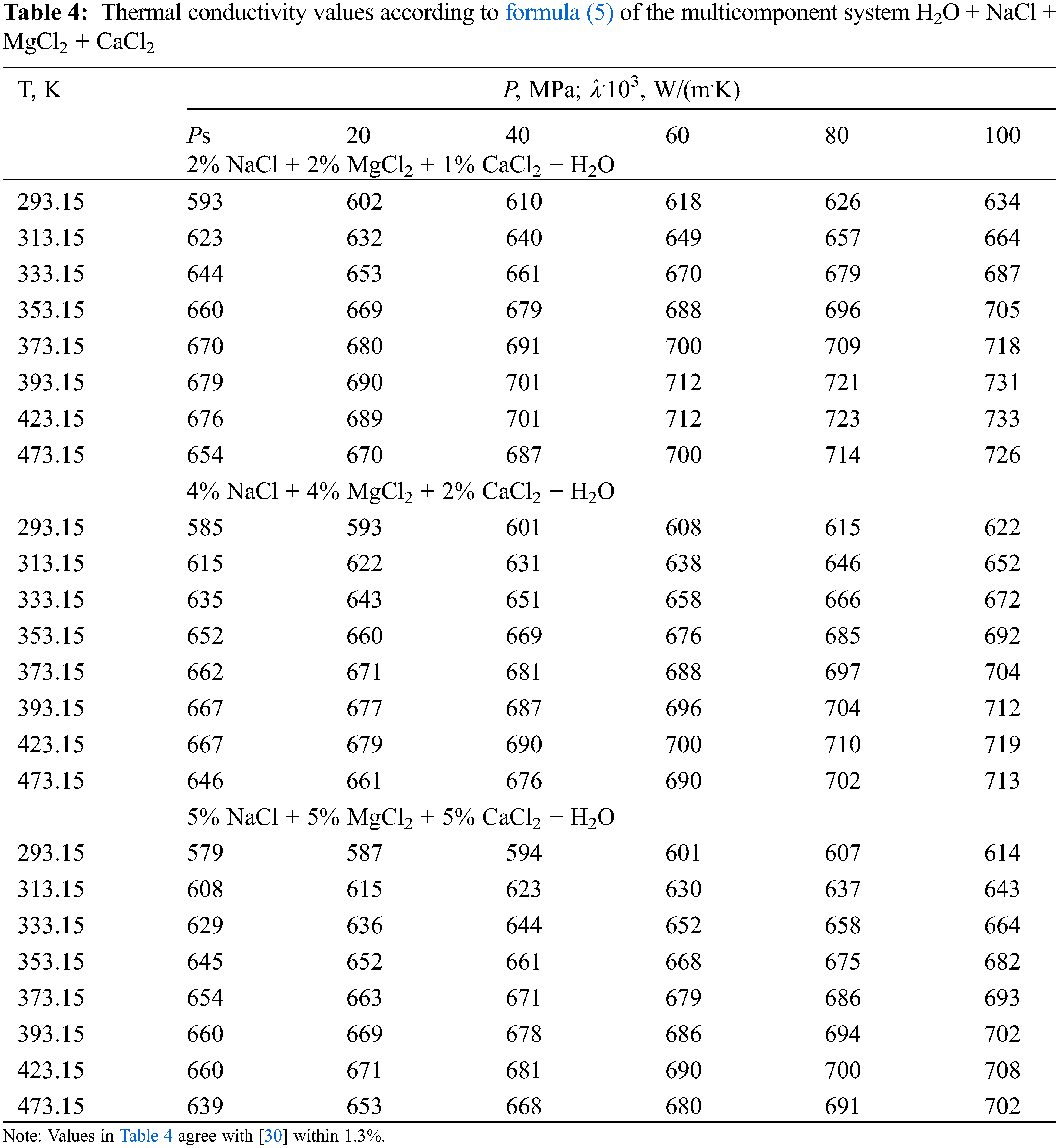
Based on the analysis of the obtained formulas and data from various works on the thermal conductivity of aqueous solutions of inorganic substances [23], a generalized formula (5) was obtained for calculating the thermal conductivity (W/(m·K)) of aqueous solutions of salts [24] in the temperature range of 293–473 K, pressures of 0.1–100 MPa, and concentrations of 0–25 wt.%.
Ai – coefficients characteristic of each binary system of aqueous solutions of inorganic substances, determined from experimental data on the thermal conductivity of the solution are presented in Table 3 and in [25–28].
Formula (6) for calculating the thermal conductivity of water and aqueous salt solutions at T = 273–473 K is presented in [30]:
and for pure water (c = 0), formula (6) takes the form of formula (7):
where Ps is the pressure near the saturation line, which during the experiment can be
Based on the analysis of the density data of pure water and experimental data on the dynamic viscosity of aqueous solutions of salts of various authors, a new generalized formula is presented that can be used to obtain the values of the viscosity of aqueous solutions of salts in the temperature range of 333–473 K, pressures of 0.1–100 MPa, and concentrations of 0–25 wt.%.
The viscosity of saline waters has not been studied sufficiently at high pressures. The material on the dynamic viscosity of water-salt systems at pressures above 40 MPa is limited. There is no reference material on the dynamic viscosity of water-salt systems at pressures of 40–100 MPa.
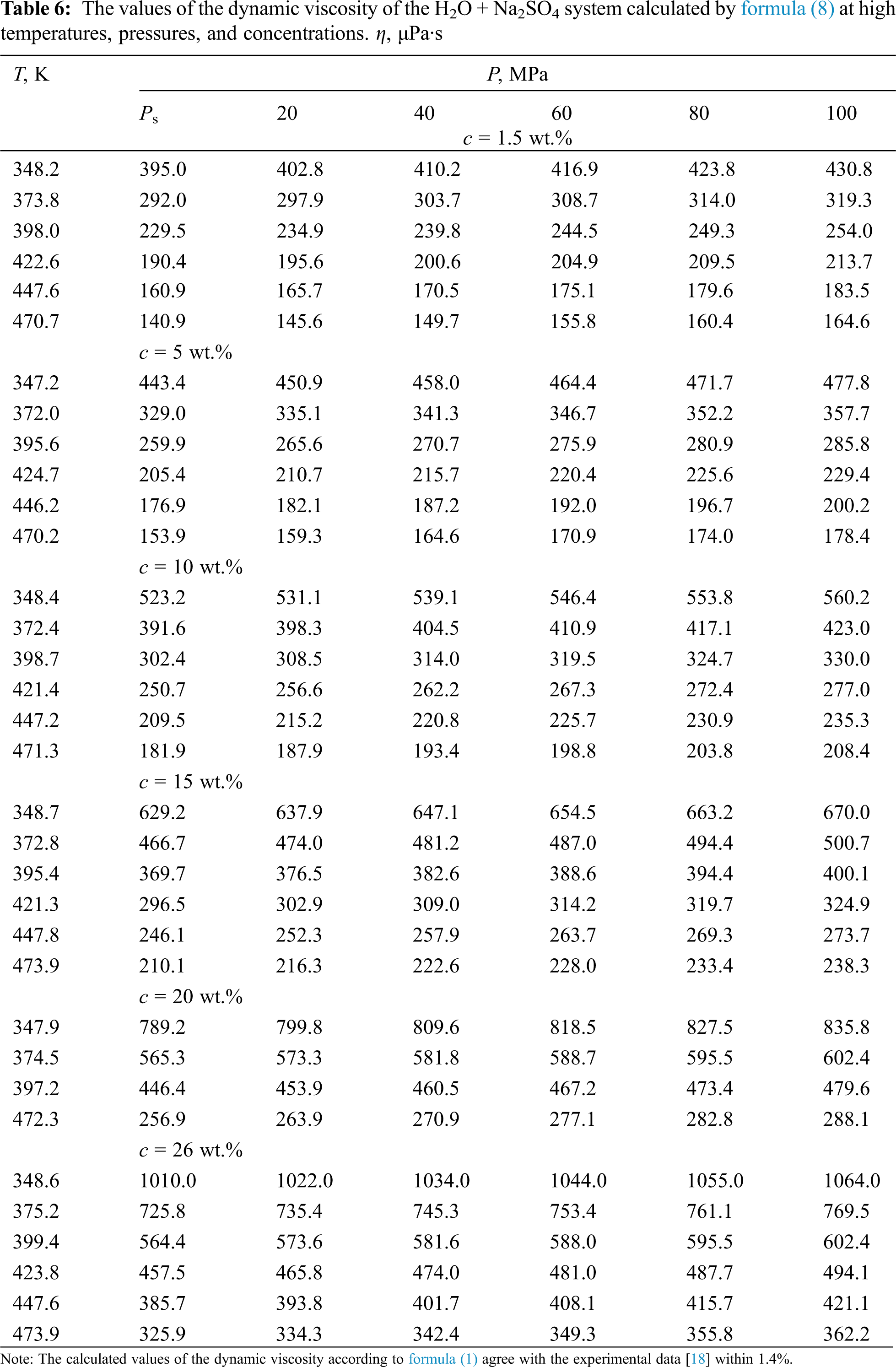
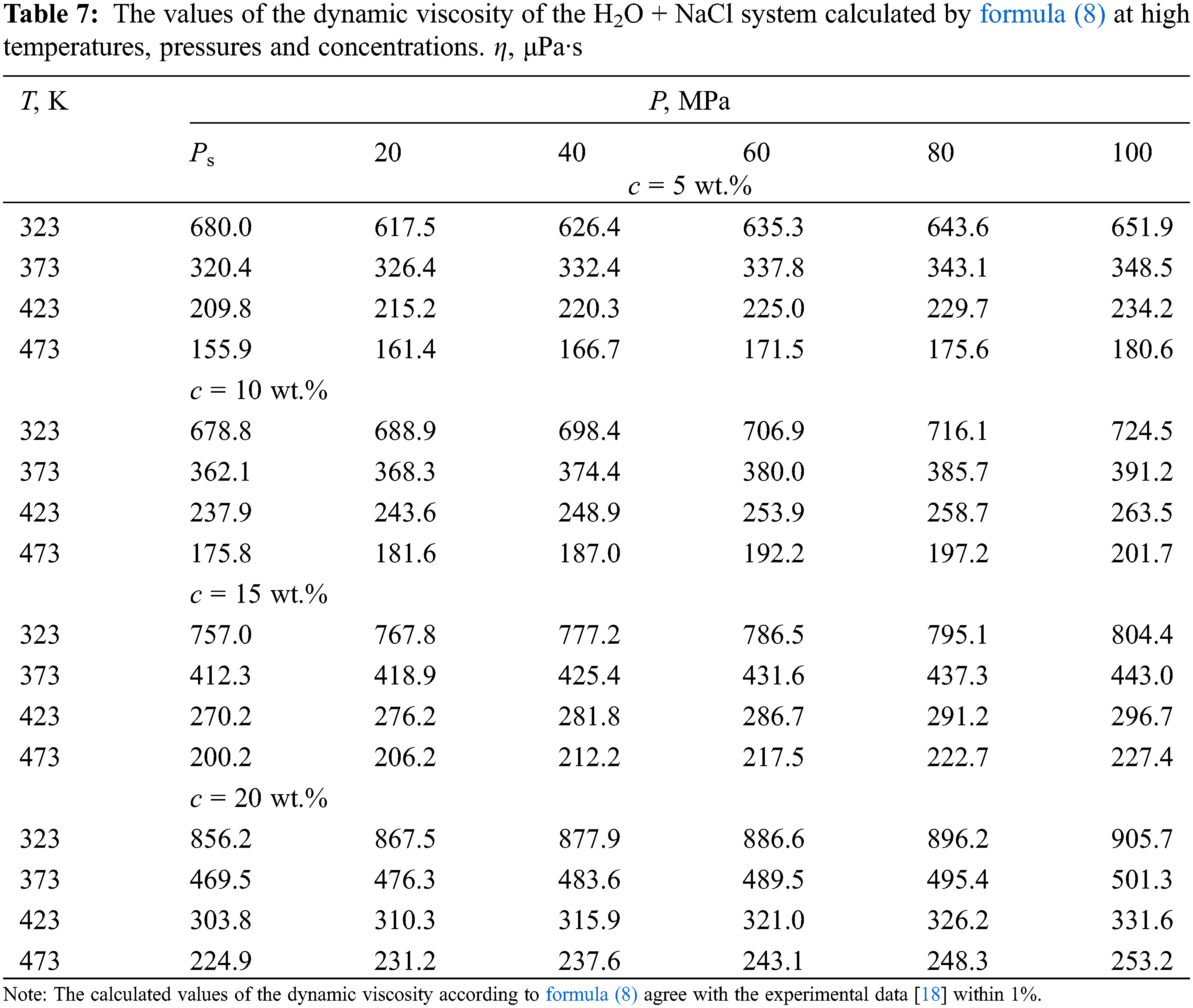
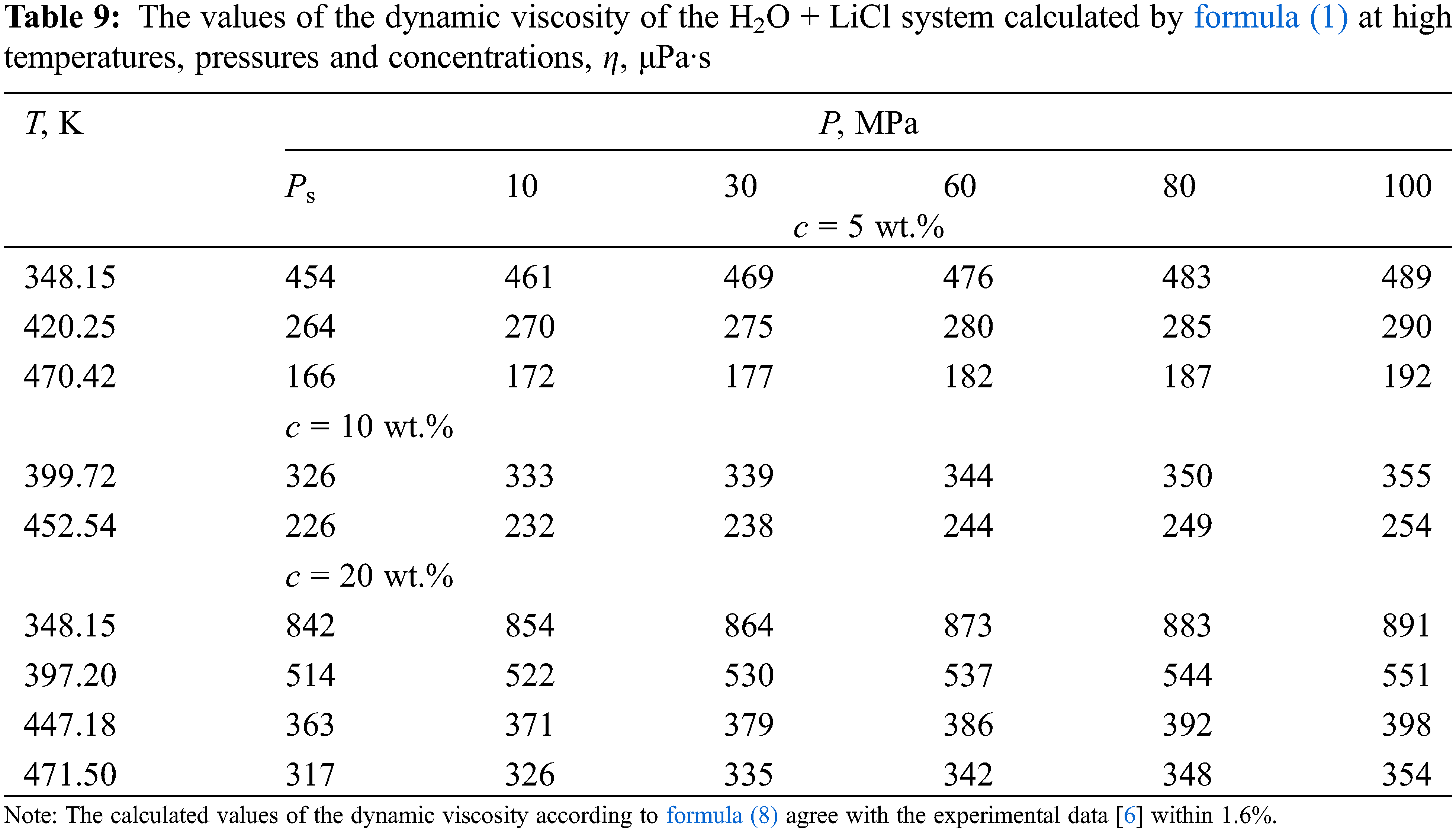
Based on the analysis of density data [31], viscosity [32] of pure water, and experimental data on the dynamic viscosity of aqueous solutions of salts of various authors [33], a new generalized formula (8) is presented, which can be used to obtain the values of viscosity (μPa·s) of aqueous solutions of salts in the temperature range of 333–473 K, pressures of 0.1–100 MPa, and concentrations of 0–25 wt.%–in the presence of viscosity data near the saturation line. The formula is as follows:
and for pure water (c = 0) formula (8) takes the form:
where
According to formula (8), the values of the dynamic viscosity of various water-salt systems were obtained in the temperature range of 333–473 K, pressures of 0.1–100 MPa, and concentrations of 0–25 wt.%. The deviation of the calculated values of the viscosity of water-salt systems according to formula (1) from the experimental data of various authors [30] was less than 1.5%. Here, in Tables 5–9, the values of dynamic viscosity for five water-salt systems are presented, although many systems have been studied, and Figs. 1 and 2 show isobars of water and aqueous solutions of sodium chloride.
Note that there are experimental studies of water-salt systems by various authors at pressures up to 40 MPa and a small part up to 60 MPa.
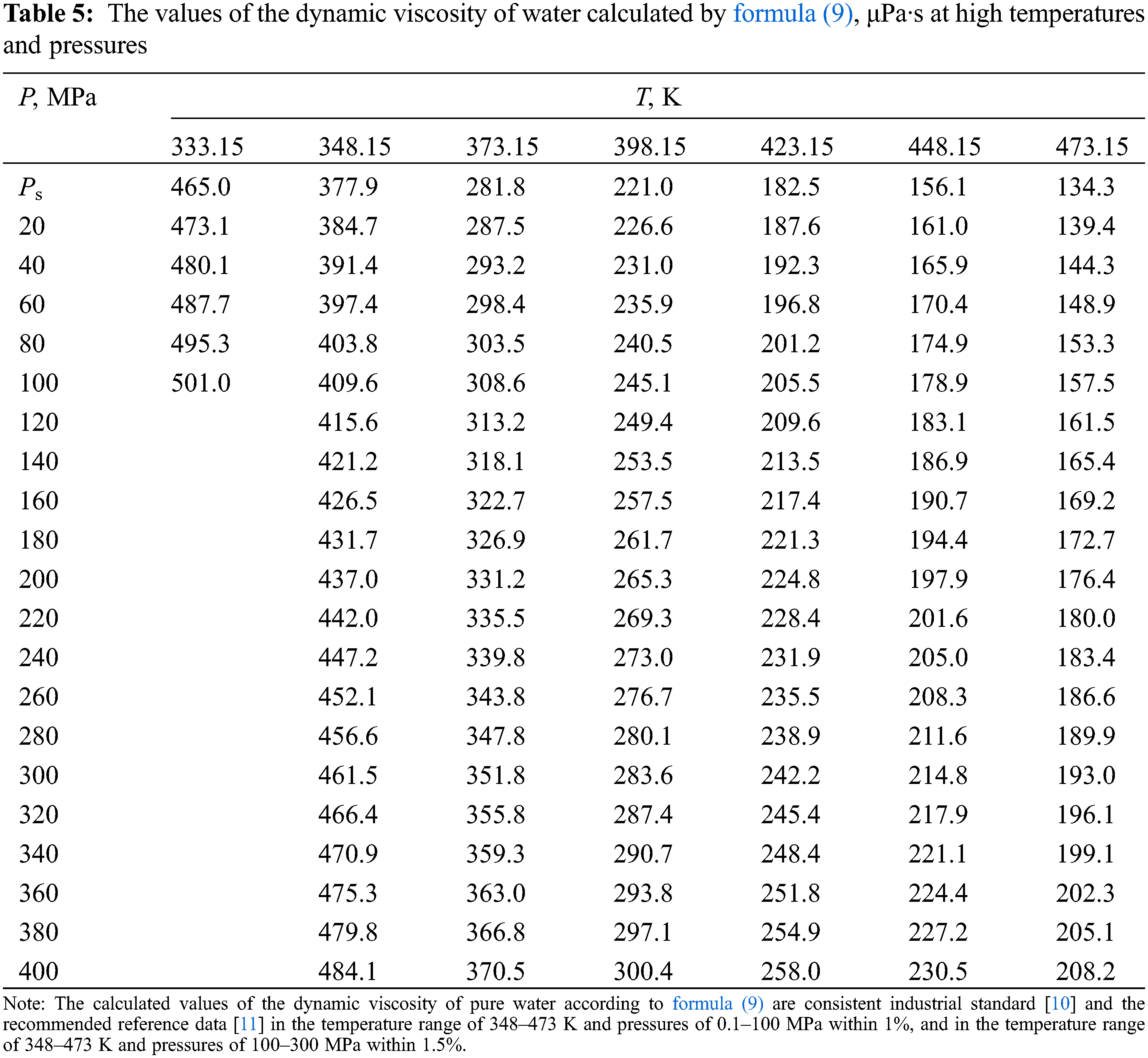
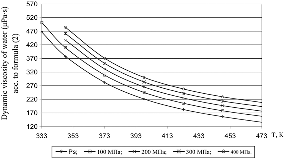
Figure 1: Viscosity of water at high state parameters
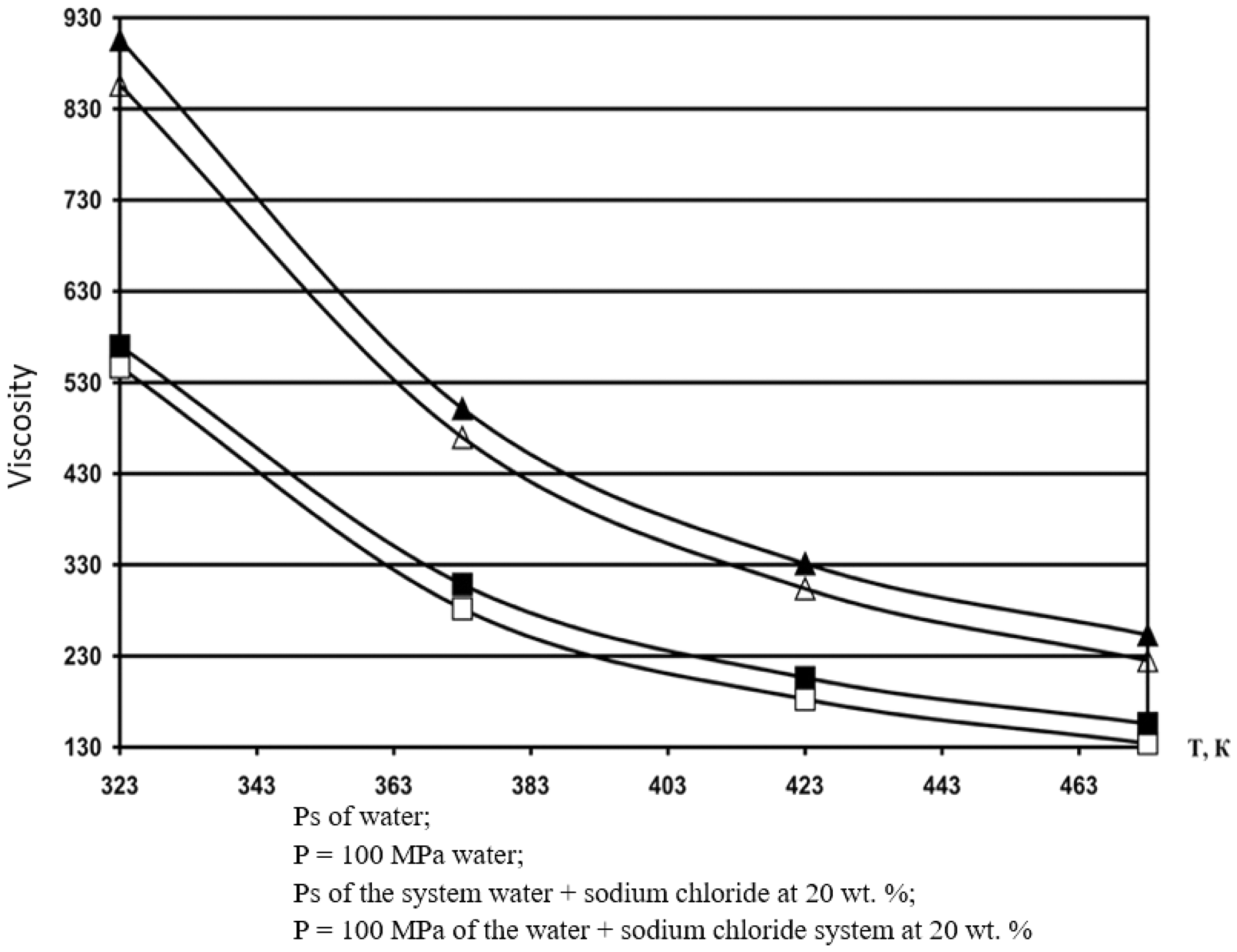
Figure 2: Isobar viscosity of water and aqueous solutions of sodium chloride, calculated by formula (1) at 20 wt.%

In the present paper Based on the analysis of experimental data, generalized formulas are presented, which in turn will allow many scientists to use them to obtain reliable and accurate material on the thermal conductivity and dynamic viscosity of aqueous solutions of salts. Nanofluids are a new generation of fluids with great potential in industrial cartridges. In nanofluids, due to the small size of the particles, a significant amount of corrosion, impurities and pressure drop problems are reduced and the stability of fluids against sedimentation is significantly improved. To increase the stability of nanofluid suspension in order to increase the thermal conductivity, surfactants and physical or chemical bonding of polymer chains on the surface of nanostructures can be used. Other factors affecting the thermal conductivity of the nanofluid include the amount of nano filler, the viscosity of the nanofluid and the temperature of the system used. The presence of nanofillers in the nanofluid changes the thermal conductivity by changing the temperature, whereas without the filler the thermal conductivity is not temperature dependent. Results demonstrated that thermal conductivity of Water hybrid nanofluid increases with increase in volume fraction of nanoparticles.Also, based on the experimental results of the previous researches a novel a novel correlation with a margin of deviation of 1.6% was proposedfor predicting thermal conductivity.
Funding Statement: The authors received no specific funding for this study.
Conflicts of Interest: The authors declare that they have no conflicts of interest to report regarding the present study.
1. Zainal, A. G., Yulianto, H., Yanfika, H. (2021). Financial benefits of the environmentally friendly aquaponic media system. IOP Conference Series: Earth and Environmental Science, vol. 739, 012024.IOP Publishing. [Google Scholar]
2. Gashi, F., Dreshaj, E., Troni, N., Maxhuni, A., Laha, F. (2020). Determination of heavy metal contents in water of Llapi River (Kosovo). A case study of correlations coefficients. European Chemical Bulletin, 9(2), 43–47. DOI 10.17628/ecb.2020.9.43-47. [Google Scholar] [CrossRef]
3. Chen, H., Bokov, D., Chupradit, S., Hekmatifar, M., Mahmoud, M. Z. et al. (2021). Combustion process of nanofluids consisting of oxygen molecules and aluminum nanoparticles in a copper nanochannel using molecular dynamics simulation. Case Studies in Thermal Engineering, 28(3), 101628. DOI 10.1016/j.csite.2021.101628. [Google Scholar] [CrossRef]
4. Prischepa, O. M., Nefedov, Y. V., Ibatullin, A. K. (2020). Raw material source of hydrocarbons of the arctic zone of russia. Periodico Tche Quimica, 17(36), 506–526. DOI 10.52571/PTQ.v17.n36.2020.521_Periodico36_pgs_506_526.pdf. [Google Scholar] [CrossRef]
5. Al-Hassani, K. A., Alam, M. S., Rahman, M. M. (2021). Numerical simulations of hydromagnetic mixed convection flow of nanofluids inside a triangular cavity on the basis of a two-component nonhomogeneous mathematical model. Fluid Dynamics & Materials Processing, 17(1), 1–20. DOI 10.32604/fdmp.2021.013497. [Google Scholar] [CrossRef]
6. Alkhasov, A. B., Magomedov, U. B., Magomedov, M. M. S. (2011). Thermal conductivity of aqueous solutions of salts at high state parameters. Natural and Technical Sciences, 1(51), 23–26. [Google Scholar]
7. Yang, S., Jasim, S. A., Bokov, D., Chupradit, S., Nakhjiri, A. T. et al. (2021). Membrane distillation technology for molecular separation: A review on the fouling, wetting and transport phenomena. Journal of Molecular Liquids, 565(2), 118115. DOI 10.1016/j.molliq.2021.118115. [Google Scholar] [CrossRef]
8. Anggono, A. D., Elveny, M., Abdelbasset, W. K., Petrov, A. M., Ershov, K. A. et al. (2021). Creep deformation of Zr55Co25Al15Ni5 bulk metallic glass near glass transition temperature: A nanoindentation study. Transactions of the Indian Institute of Metals, 1–8. [Google Scholar]
9. Nourdanesh, N., Ranjbar, F. (2022). Investigation on heat transfer performance of a novel active method heat sink to maximize the efficiency of thermal energy storage systems. Journal of Energy Storage, 45(12), 103779. DOI 10.1016/j.est.2021.103779. [Google Scholar] [CrossRef]
10. Nourdanesh, N., Ranjbar, F. (2021). Introduction of a novel electric field-based plate heat sink for heat transfer enhancement of thermal systems. International Journal of Numerical Methods for Heat & Fluid Flow, 61. DOI 10.1108/HFF-08-2021-0531. [Google Scholar] [CrossRef]
11. Magomedov, U. B. (2005). Thermal conductivity of aqueous solutions of inorganic substances at high temperatures, pressures and concentrations. Materials of the International Conference Renewable Energy: Problems and Prospects, vol. 2, pp. 115–123. Makhachkala: Delovoi mir. [Google Scholar]
12. Mozaffari, M., D’Orazio, A., Karimipour, A., Abdollahi, A., Safaei, M. R. (2019). Lattice Boltzmann method to simulate convection heat transfer in a microchannel under heat flux: Gravity and inclination angle on slip-velocity. International Journal of Numerical Methods for Heat & Fluid Flow, 30(6), 3371–3398. DOI 10.1108/HFF-12-2018-0821. [Google Scholar] [CrossRef]
13. Abdulagatov, I. M., Azizov, N. D. (2006). Viscosity of aqueous calcium chloride solutions at high temperatures and high pressures. Fluid Phase Equilibria, 240(2), 204–219. DOI 10.1016/j.fluid.2005.12.036. [Google Scholar] [CrossRef]
14. Sun, K., Hu, X., Li, D., Zhang, G., Zhao, K. et al. (2021). Analysis of bubble behavior in a horizontal rectangular channel under subcooled flow boiling conditions. Fluid Dynamics & Materials Processing, 17(1), 81–95. DOI 10.32604/fdmp.2021.013895. [Google Scholar] [CrossRef]
15. Han, Y. (2020). Investigation of reynolds number effects on high-speed trains using low temperature wind tunnel test facility. Fluid Dynamics & Materials Processing, 16(1), 1–19. DOI 10.32604/fdmp.2020.06525. [Google Scholar] [CrossRef]
16. Abdulagatov, I. M., Azizov, N. D. (2005). Viscosity of aqueous LiI solutions at 293-523 K and 0.1–40 MPa. Thermochimica Acta, 439(1–2), 8–20. DOI 10.1016/j.tca.2005.08.036. [Google Scholar] [CrossRef]
17. Abdulagatov, I. M., Zeinalova, A. B., Azizov, N. D. (2004). Viscosity of the aqueous Ca (NO3)2 solutions at temperatures 298 to 573 K and at pressures up to 40 MPa. Journal of Chemical Engineering Data, 49(5), 1444–1450. DOI 10.1021/je049853n. [Google Scholar] [CrossRef]
18. Abdulagatov, I. M., Zeinalova, A. B., Azizov, N. D. (2006). Experimental viscosity B-coefficients of aqueous LiCl solutions. Journal of Molecular Liquids, 126(1–3), 75–88. DOI 10.1016/j.molliq.2005.10.006. [Google Scholar] [CrossRef]
19. Akmedova-Azizova, L. A. (2006). Thermal conductivity and viscosity of aqueous Mg(NO3)2, Ca(NO3)2 and Ba(NO3)2 solutions at high temperatures and high pressures. Journal of Chemical Engineering Data, 54, 510–517. [Google Scholar]
20. Tian, Z., Bagherzadeh, S. A., Ghani, K., Karimipour, A., Abdollahi, A. et al. (2019). Nonlinear function estimation fuzzy system (NFEFS) as a novel statistical approach to estimate nanofluids’ thermal conductivity according to empirical data. International Journal of Numerical Methods for Heat & Fluid Flow, 30(6), 3267–3281. DOI 10.1108/HFF-12-2018-0768. [Google Scholar] [CrossRef]
21. Hoseini, M., Haghtalab, A., Navid Family, M. (2020). Elongational behavior of silica nanoparticle-filled low-density polyethylene/polylactic acid blends and their morphology. Rheologica Acta, 59(9), 621–630. DOI 10.1007/s00397-020-01225-5. [Google Scholar] [CrossRef]
22. Abdulagatov, I. M., Zeinalova, A. B., Azizov, N. D. (2005). Viscosity of aqueous Na2SO4 solutions at temperatures from (298 to 573) K and at pressures up to 40 MPa. Fluid Phase Equilibria, 227(1), 57–70. DOI 10.1016/j.fluid.2004.10.028. [Google Scholar] [CrossRef]
23. Zeynalova, A. B., Iskenderov, A. I., Tairov, A. D., Akhundov, T. S. (1991). Dynamic viscosity of calcium nitrate. Oil and Gas Studies, 1, 53–54. [Google Scholar]
24. Nikfarjam, A., Raji, H., Hashemi, M. M. (2019). Label-free impedance-based detection of encapsulated single cells in droplets in low cost and transparent microfluidic chip. Journal of Bioengineering Research, 1(4), 29–37. [Google Scholar]
25. Ahmadizadeh, P., Mashadi, B., Lodaya, D. (2017). Energy management of a dual-mode power-split powertrain based on the Pontryagin’s minimum principle. IET Intelligent Transport Systems, 11(9), 561–571. DOI 10.1049/iet-its.2016.0281. [Google Scholar] [CrossRef]
26. Sokolov, B., Potryasaev, S., Serova, E., Ipatov, Y., Andrianov, Y. (2019). Informative and formal description of structure dynamics control task of cyber-physical systems. Journal of Applied Engineering Science, 17(1), 61–64. DOI 10.5937/jaes16-18716. [Google Scholar] [CrossRef]
27. Bakhtiari, R., Kamkari, B., Afrand, M., Abdollahi, A. (2021). Preparation of stable TiO2-Graphene/Water hybrid nanofluids and development of a new correlation for thermal conductivity. Powder Technology, 385, 466–477. DOI 10.1016/j.powtec.2021.03.010. [Google Scholar] [CrossRef]
28. Deryagin, A. V., Krasnova, L. A., Sahabiev, I. A., Samedov, M. N., Shurygin, V. Y. (2019). Scientific and educational experiment in the engineering training of students in the bachelor’s degree program in energy production. International Journal of Innovative Technology and Exploring Engineering, 8(8), 572–577. [Google Scholar]
29. Kuzmin, P. A., Bukharina, I. L., Kuzmina, A. M. (2016). The activity of copper-containing enzymes in the birch leaves in the conditions of the built environment. International Journal of Pharmacy and Technology, 8(4), 24608–24614. [Google Scholar]
30. Fedorov, S. N., Smolnikov, A. D., Palyanitsin, P. S. (2020). Metrology and standardization in pressureless flows. Journal of Physics: Conference Series, 1515(5), 052069. DOI 10.1088/1742-6596/1515/5/052069. [Google Scholar] [CrossRef]
31. Movchan, I. B., Yakovleva, A. A., Daniliev, S. M. (2019). Parametric decoding and approximated estimations in engineering geophysics with the localization of seismic risk zones on the example of northern part of kola peninsula. 15th Conference and Exhibition Engineering and Mining Geophysics, pp. 188–198. Gelendzhik. [Google Scholar]
32. He, W., Bagherzadeh, S. A., Tahmasebi, M., Abdollahi, A., Bahrami, M. et al. (2019). A new method of black-box fuzzy system identification optimized by genetic algorithm and its application to predict mixture thermal properties. International Journal of Numerical Methods for Heat & Fluid Flow, 30(5), 2485–2499. DOI 10.1108/HFF-12-2018-0758. [Google Scholar] [CrossRef]
33. Gerdroodbary, M. B., Ganji, D. D., Moradi, R., Abdollahi, A. (2018). Application of knudsen thermal force for detection of CO2 in low-pressure micro gas sensor. Fluid Dynamics, 53(6), 812–823. DOI 10.1134/S0015462818060149. [Google Scholar] [CrossRef]
 | This work is licensed under a Creative Commons Attribution 4.0 International License, which permits unrestricted use, distribution, and reproduction in any medium, provided the original work is properly cited. |