Fluid Dynamics & Materials Processing

DOI: 10.32604/fdmp.2022.019810

ARTICLE

A Mathematical Model of Heat Transfer in Problems of Pipeline Plugging Agent Freezing Induced by Liquid Nitrogen

Yafei Li and Yanjun Liu*

Southwest Petroleum University, Chengdu, 610500, China
*Corresponding Author: Yanjun Liu. Email: SWPUliuyanjun@126.com
Received: 16 October 2021; Accepted: 28 December 2021

Nomenclature

1  Introduction

In the gas pipelines industry, due to the factors such as corrosion, topography and process transformation, it is often necessary to replace the pipes or valves, or change the line [1]. Emergency repair operations likes these usually have to vent the natural gas in a long pipe section and replacing them with nitrogen. Then non-spark cutting equipment is required to cut it off, and finally, operators could conduct their assignment with the help of welding [2]. This method is very safe, but high-cost and time-consuming, which is not environmentally friendly yet [3].

Therefore, a more economical and safer way plugging–both ends of the problematic pipe section–was raised, which could reduce the waste by venting less gas. At present, the commonly technique for gas pipeline plugging includes mechanical plugging and bladder plugging [4]. The former one is good at plugging [5], but non-economic and complex in operation [6]. The latter spends less while its blocking effect is poor [7]. The pipeline freezing and plugging technique, which not only costs less but also performs better in plugging, was first proposed by Bishop et al. [8]. This method could freeze the fluid by implementing part refrigeration outside the pipe to form a frozen plug, with low cost and good plugging performance [9]. Burton et al. [10] was the one who observed and analyzed the water’s natural convection phenomenon in the pipe during refrigeration, and Keary [11] was the one who simulated the cooling and freezing process of the flowing water in the pipe, and Bueno et al. [12] successfully froze the crude oil pipeline. In early times, it was considered that the pipeline freezing and plugging technique is only applicable to pipelines where the medium in the pipe was liquid. The reason for this idea is that the gas cannot be frozen, besides, injecting freezable fluid into the pipeline could not fill the pipe section to form a closed freezing plug. Afterwards Zhang et al. suggested to restrict the fluid plugging agent by using the airbag, whose expansion are able to generate pressure with the inner wall of the pipe, resulting in axial static friction, so that the fluid plugging agent can fill the pipe (Fig. 1). Wang et al. [13] and Liang et al. [14] conducted experiments to test the plugging performance of different diameter natural gas pipelines.

Nowadays, most researches focus on the pressure-bearing capacity of the freezing plug, which is to put the prefabricated freezing plug into the cut pipeline for freezing, and then test the pressure. Liang et al. [14] conducted a pressurization experiment on an 86 mm small-diameter natural gas pipeline. Wang et al. [13] did the same experiment on a 762 mm large-diameter natural gas pipeline. The pressure-bearing capacity of the plugging proves the feasibility of applying the freezing and plugging technique to natural gas pipelines. The actual pipeline freezing and plugging, however, is carried out in a closed pipe, and it is impossible to cut the pipeline and put the freezing plug into it. Therefore, it is particularly significant to study the heat transfer characteristics of the pipeline’s freezing and plugging. Learning the heat transfer process can help researchers predict the formation of freezing plugs in closed pipelines, which lays a foundation for the research on the influence of heat transfer factors on the pressure bearing capacity of freezing plugs. However, it is barely studied.

Based on the status quo, the objectives of this study are:

(1) Develop a transient temperature field model and phase change model of the one-dimensional circular pipe of freezing and plugging;

(2) Conduct experiments to confirm the model;

(3) Extend the model to practical engineering–predicting the time for the freezing plug to form.

Figure 1: Freezing and plugging technique for gas pipeline

2  Heat Transfer Modeling

2.1 Physical Model

When freezing, one jacket is needed to set outside the pipe so that liquid nitrogen can be introduced to freeze the plugging agent. At the same time, it is requested for two special airbags at the both end of the pipe to limit the plugging agent in the pipe section, so it can be frozen to an airtight freezing plug. In order to simplify the physical model, it is assuming that:

(1) Both ends of the plugging agent are thermal insulation during the freezing and plugging process;

(2) The radial temperature of the outer wall of the pipe section in the jacket is uniform;

(3) The axial temperature distribution in the refrigeration zone is uniform;

(4) Ignoring the natural convection effect of the fluid due to the density change caused by refrigeration.

According to these assumptions above, this model can be applied when the jacket length is greater than three times the pipe diameter and liquid nitrogen is used as refrigerant. And if the density of plugging agent changes greatly due to the difference in temperature, the natural convection effect needs to be taken into account.

As shown in Fig. 2, the simplified model only considers the one-dimensional transient heat transfer in the radial direction of the pipe.

Then, based on this physical model, it is possible to analyze and build a cooling model for the plugging agent from liquid to freezing point and a freezing model from freezing point to solid.

Figure 2: Physical model of heat transfer in pipeline freezing plugging

2.2 Cooling Model

Before cooling, the liquid plugging agent will be cooled from its initial temperature to its freezing point at the refrigeration temperature. The governing equation of the liquid temperature, T(r,t) , in the tube during this process is:

∂2T∂r2+1r∂T∂r=1α∂T(r,t)∂t0 ≤ r ≤ Rinn,t>0 (1)

The boundary condition and initial condition are as follows:

−kL∂T(r,t)∂r=U[T(r,t)−T∞]r=Rinn (2)

T(r,t)=Ti−T∞t=0,0 ≤ r ≤ Rinn (3)

where U is total heat transfer coefficient, calculated as follows:

1U=R′′+1ho (4)

where R′′ is:

R′′=itln(DoDinn)2kpDo (5)

Liquid nitrogen will rapidly vaporize and expand in the jacket. And the state of nitrogen sweeping the pipe wall is very complicated, so it is hard to obtain the precise value of the convective heat transfer coefficient of the outer wall of the pipe. Perkins et al. [15], who found the average heat transfer coefficient will be affected by the flow in the laminar boundary layer and the separation area on the tube, derived the equation for estimating the average heat transfer coefficient on the cylinder:

ho=kNDo[0.31Re0.50+0.11Re0.67]Pr0.40 (6)

Decompose T(r,t) by separating variables:

T(r,t)=R(r)Γ(t) (7)

Incorporating Eq. (7) into Eq. (1):

1R(r)(d2R(r)dr2+1rdR(r)dr)=1αΓ(t)dΓ(t)dt (8)

In this equation, the left side is about the space, and the right side is about the time, then there is:

1R(r)(d2R(r)dr2+1rdR(r)dr)=1αΓ(t)dΓ(t)dt=−λ2 (9)

λ is eigenvalue, then:

dΓ(t)dt+αλ2Γ(t)=0 (10)

d2R(r)dr2+1rdR(r)dr+λ2R(r)=0 (11)

By solving the Eq. (10), the following equation is obtained:

Γ(t)=e−αλ2t (12)

Eq. (11) is the zero-order Bessel equation. The defined problem is called eigenvalue problem. It can obtain solution only when λ=λm,m=1,2,3… , so, R(r) is related to λm and becomes R(λm,r) . The solution of R(λm,r) is composed of the first kind of zero-order Bessel function J0(λm,r) and the second kind of zero-order Bessel function Y0(λm,r) . When r = 0, Y0(λm,r) is infinite, so the finite value solution at r = 0 is taken as:

R(λm,r)=J0(λmr) (13)

If Eq. (13) satisfies the boundary condition Eq. (2), then the eigenvalue λm is the positive root of the following transcendental equation:

λmJ0′(λmRinn)+UJ0(λmRinn)/kL=0 (14)

The complete solution of the temperature, T(r,t) , can be formed by the basic solution of the separation equation containing variables according to the principle of linear superposition, and its form is:

T(r,t)=∑m=1∞cme−αλm2tR(λm,r) (15)

Bring initial condition Eq. (3) into Eq. (15):

T(r,0)=∑m=1∞cmR0(λm,r) (16)

The unknown coefficient cm can be determined according to the orthogonality of the characteristic function R(λm,r) :

∫0RinnrR(λn,r)R(λm,r)dr={0m≠nN(λm)m=n (17)

Then use the operator ∫0RinnrR(λm,r)dr to operate on both sides of Eq. (16), and combined Eq. (17), it can get:

cm=1N(λm)∫0RinnrR(λm,r)F(r)dr (18a)

N(λm)=∫0RinnrR2(λm,r)dr (18b)

Bring the value of cm into Eq. (15), and use the properties of Bessel function to obtain the final form of T(r,t) :

T(r,t)=T∞+2u(Ti−T∞)Rinn∑m=1∞e−αλm2tJ0(λmr)(λm2+u2)J0(λmRinn) (19)

Eq. (19) is a heat transfer model with a space variable r and a time variable t , which can obtain the transient temperature field in a one-dimensional tube when the plugging agent is liquid.

2.3 Freezing Model

When the plugging agent undergoes a phase change, it can be considered that the solid phase and the liquid phase are at the same temperature, thus the focus should lie in the movement of the solid phase and the liquid phase. The governing equations for the temperature distribution of solid phase and liquid phase are as follows:

TL(r,t)=Tf0≤r<rin(t) (20)

1r∂∂r(r∂Ts∂r2)=1αs∂Ts∂trin(t)<r≤Rinn (21)

The boundary condition and initial condition are as follows:

Ts(rin,t)=Tfr=rin (22)

−ks∂Ts(r,t)∂r=U[Ts(r,t)−T∞]r=Rinn (23)

Ts(r,t)=Tft=0 (24)

rin(t)=Rinnt=0 (25)

The phase change is accompanied by the movement of the solid-liquid interface. Due to the energy conservation of the solid-liquid interface, another boundary condition–the interface energy equation–will produce. rin(t) is the transient position of the interface, and the energy equation of the solid-liquid interface is:

ks∂Ts(r,t)∂r=ρsLdrdtr=rin (26)

Eq. (21) can be solved by variable separation [16]. And Eq. (21) together with Eq. (25) determine the inhomogeneity of Ts(r,t) , so it can be assumed that the solution of Ts(r,t) is the sum of two functions. One is a general solution to r and t, Ψ(r,t) , and another is special solution for r, ϕ(r) , then:

Ts(r,t)=Ψ(r,t)+ϕ(r) (27)

Incorporating Eq. (27) into Eq. (21):

1r∂∂r(r∂Ψ∂r)=1αs∂Ψ∂t (28)

1rddr(rdϕdr)=0 (29)

Decompose Ψ(r,t) as following:

Ψ(r,t)=ℜ(r)τ(t) (30)

where:

ℜ(r)=AkJ0(λkr)+BkY0(λkr) (31)

τ(t)=Cke−αsλk2t (32)

where Ak , Bk and Ck are integral constants; λk is the eigenvalue. In order to determine λk , the boundary condition Eq. (23) is incorporated into Eq. (31):

λk[J1(λkRinn)−J0(λkrin)Y0(λkrin)Y1(λkRinn)][J0(λkRinn)−J0(λkrin)Y0(λkrin)Y0(λkRinn)]=Uks (33)

One of the values of λk is λk=λ0=0 . Put λ0 into Eqs. (31) and (32), and then put boundary conditions (22) and (23) into Eq. (31):

Ψ(r,t)=ℜ(r)τ(t)=0ℜ(r)=0 (34)

Then the solution of Ψ(r,t) is

Ψ(r,t)=∑k=1∞ak[J0(λkr)−J0(λkrin)Y0(λkrin)Y0(λkr)]e−αsλk2t (35)

where ak=AkCk .

By solving Eq. (29):

ϕ(r)=Eln r+F (36)

where E and F are integral constants. Bring the boundary conditions Eqs. (22) and (23) into Eq. (36):

E=U(Tf−T∞)Uln(rinRinn)−ksRinn (37a)

F=Tf−U(Tf−T∞)Uln(rinRinn)−ksRinnln rin (37b)

Then introduce E and F into ϕ(r) , and ϕ(r) into Eq. (27). It can be achieved that the temperature distribution in the solid phase is:

Ts(r,t)−Tf=U(Tf−T∞)Uln⁡(rinRinn)−ksRinnln⁡(rrin)+∑k=1∞ak[J0(λkr)−J0(λkrin)Y0(λkrin)Y0(λkr)]e−αsλk2t (38)

Putting Eq. (38) into the energy Eq. (26):

[U(Tf−T∞)rin[Uln⁡(rinRinn)−ksRinn]+∑k=1∞akλk[J0(λkrin)Y0(λkrin)Y1(λkrin)−J1(λkrin)]e−αsλk2t]ks≈ρsLdrindt (39)

Then different eigenvalues λk can be brought into Eq. (39) by using Matlab. Through first-order finite difference approximate estimation, it is found that the approximate value of the first term dominated by the summation term of infinite series is 10−7 , then:

ksU(Tf−T∞)rin[Uln(rinRinn)−ksRinn]≈ρsLdrindt (40)

Eq. (40) gives the position changes of t the solid-liquid interface over time under the condition of radial axis symmetry in the pipeline, which could be used to predict whether the freezing and plugging is accomplished.

3  Experiment

3.1 Experiment System

In order to verify the heat transfer model, one freezing and plugging experiment system with a 219 mm long pipeline was designed and built. As it is shown in Fig. 3, the system includes experimental pipelines, refrigeration jackets, liquid nitrogen delivery devices, temperature data collection devices, pressurizing devices, pressure monitoring devices and related accessories. The parameters are shown in Table 1.

Figure 3: Pipe freezing and plugging experimental system

3.2 Experimental Method

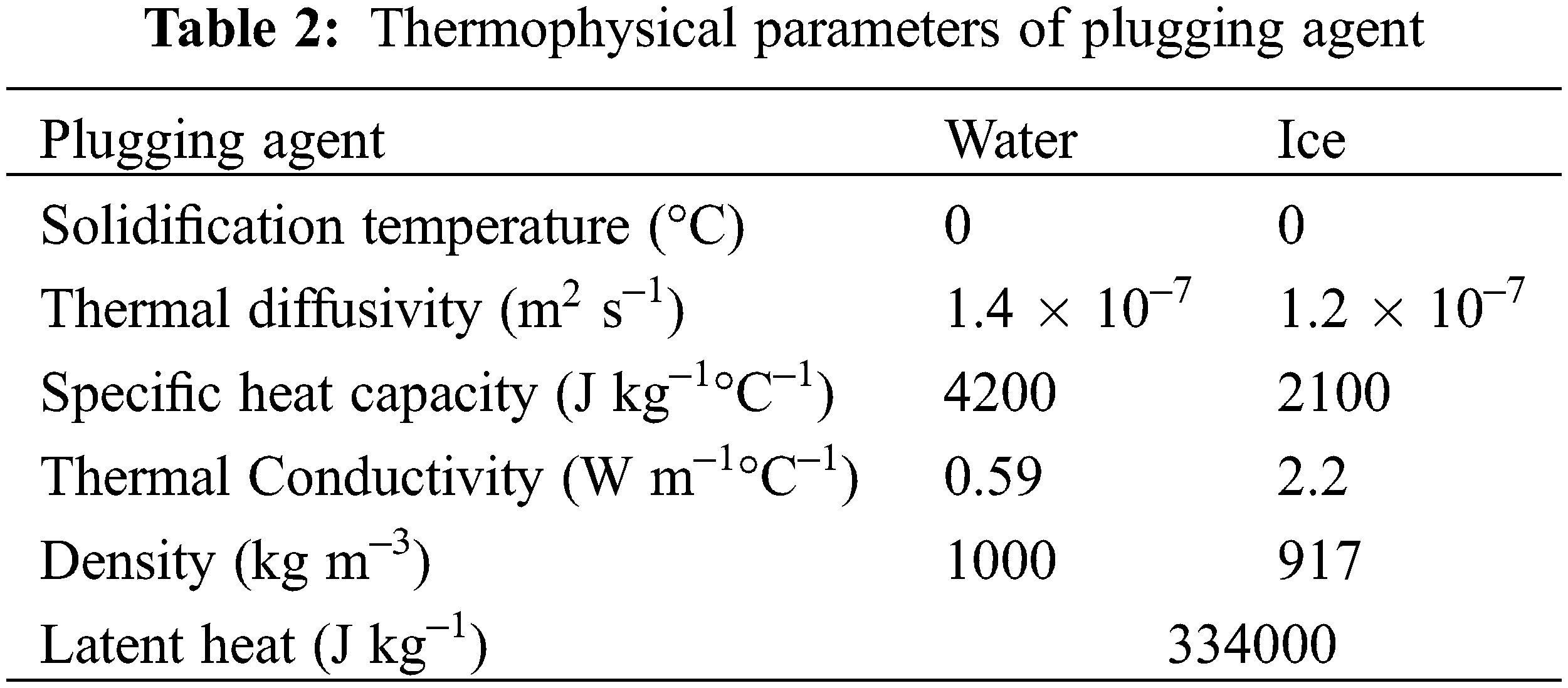
Generally, water or solid water emulsifier [13] is used as the plugging agent when freezing and plugging gas pipelines. This experiment takes water as the plugging agent, and the thermal physical parameters [17] of which are in Table 2.

Firstly, the pipe will be filled with water to replace the gas. Secondly, all valves of the pipe will be closed. Then, we press 5 MPa into the pipe through a nitrogen bottle and last for 30 min. The tightness of the experimental system can be determined by observing whether there is water seepage at the pipe wall, joints or welds. After the test, the pressure can be released.

At the beginning of the experiment, we can inject the plugging agent into the pipe through Nipple.1 until the pipe is full. Then the liquid nitrogen tank valve 1 will be opened to transport the liquid nitrogen through Nipple.3 to refrigerate. A temperature sensor is installed at the nitrogen’s outlet Nipple.2 to measure the refrigeration temperature, which is adjusted by the flow change of the liquid nitrogen. In this system, 5 groups of different refrigeration temperatures are set within the range of –30°C to –71°C. The temperature of the plugging agent is measured by the temperature sensor set at the center of the pipeline. These data, which will be gathered every 1 s, will be collected by the XMT624 intelligent PID device, and recorded by a computer. At both ends of the jacket, the pipe is filled with thermal insulation materials to simulate the airbag to limit the position of the plugging agent. The pipe and refrigeration jacket are equipped with insulation layers to reduce the outside interference.

Once the temperature in the center of the pipeline reaches below 0°C, it can be considered that the freezing plug is completely closed [18]. Then we can open the pressurizing device to pressurize the pipe from 0 MPa to 2 MPa through Nipple.3. Nipple.1 on the other side of the pipeline is in the normally open state. If the freezing plug is not entirely closed, there will be gas or plugging agent overflow from Nipple.1. If not, we can conclude that the freezing plug is formed. Then the freezing model can be verified by whether the freezing plug is closed and the time it cost.

4  Results and Discussion

4.1 Experiment Result

When the average refrigeration temperature, T∞ , of liquid nitrogen is –30.4°C, –41.3°C, –52.1°C, –60.8°C and –70.2°C, the temperature change of the plugging agent is shown in Fig. 4. It can be seen that the temperature of the plugging agent shows a downward-steady-downward trend. This is because at the first stage, the plugging agent will gradually cool down to its freezing point under the action of liquid nitrogen, during which the plugging agent will remain in a liquid state. Then the plugging agent will begin to release latent heat and freeze, and the solid-liquid interface will gradually move from the pipe wall to the center of the pipe until the plugging agent is completely frozen. In this period, the temperature is almost constant. After the plugging agent was entirely frozen, it will continue cooling down in the solid-state, which is similar to the heat transfer process of frozen soil [19].

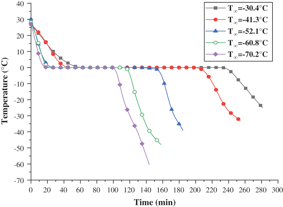
Figure 4: Temperature change of plugging agent at different refrigeration temperatures

The cooling, freezing time, and cooling rate of the plugging agent in the 5 groups of experiments are shown in Table 3.

4.2 Model Verification

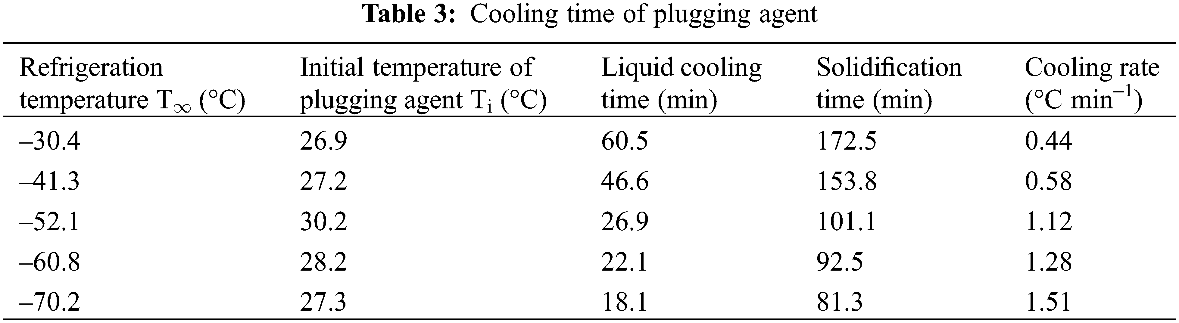
The cooling and freezing time of the plugging agent in the pipeline depends on the transient temperature distribution of the liquid and solid phases. The temperature distribution model Eqs. (19) and (40) are used to estimate the cooling and freezing time of the plugging agent respectively. The total heat transfer coefficient, U, which is the main parameter needed to be determined, is calculated by Eqs. (4)–(6). The value of U at different liquid nitrogen refrigeration temperatures are shown in Table 4.

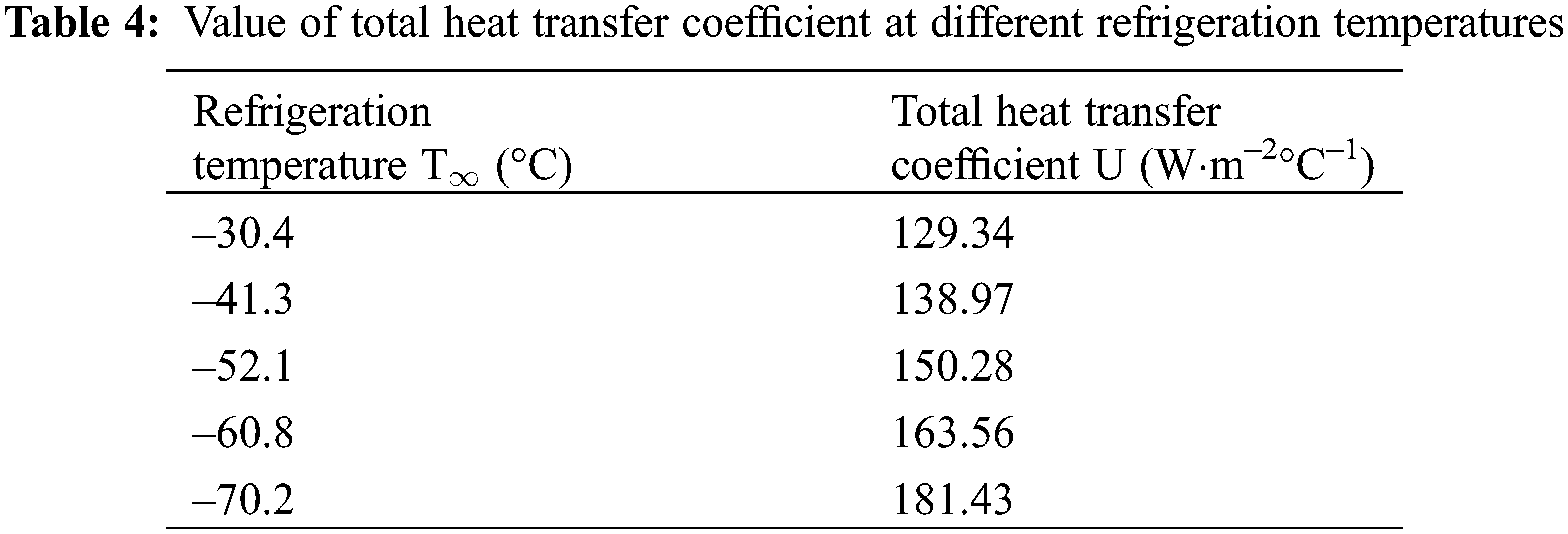
Put the value of U into Eqs. (19) and (40) to get the model result. The comparison between the model calculation value and the experiment is shown in Fig. 5. As shown in Fig. 5a, the error between theoretical value and actual value is large when the plugging agent was cooled from the liquid state to the freezing point. The minimum error is 25.41%, and the maximum is 50.92%. The reason for this phenomenon is that because when cooling, the temperature of the plugging agent near the pipe wall is low, while near the center of the pipe is relatively high. The uneven density of the plugging agent caused by the temperature will cause a small but complex convection effect [20], which enhanced the heat transfer effect [21]. Fig. 5b shows that the average error between the model and the experiment is 13.91% during the freezing process. As shown in Fig. 5c, the average error of the total time (liquid cooling time plus freezing time) between the heat transfer model and the experiment is just 17.18%. So, it can be considered that the model agreed with the experimental results.

In the cooling stage, the error between the model and the experiment is at the range of 25.41%–50.92%. This mainly caused by the ignorance of the natural convection of the refrigerant in the tube. As the cooling temperature of liquid nitrogen decreases, the convective heat transfer coefficient outside the tube increases and the error is gradually reduced, which indicates that the effect of forced convection outside the tube is stronger than the natural convection inside.

At the freezing stage, the maximum error between the model and the experiment is 15.23%, and the minimum is 7.81%. The lower the liquid nitrogen refrigeration temperature, the smaller the error is. The main cause of the error is that the process of vaporization and expansion of liquid nitrogen in the jacket is complicated, and the convective heat transfer coefficient estimated by the model is different from the real situation. The overall average error between the experiment and the model is 17.18%, which includes the error of the cooling stage and the freezing stage. Although the error of the cooling stage is relatively large, it accounts for a small proportion in the overall time. It is the freezing phase that controls the main error. As the refrigeration effect of liquid nitrogen increases, the overall error shows a decreasing trend. The model uses the outlet end temperature of the refrigeration jacket to represent the average refrigeration temperature of the jacket, which leads that the date of the heat transfer model is more conservative than the experimental results.

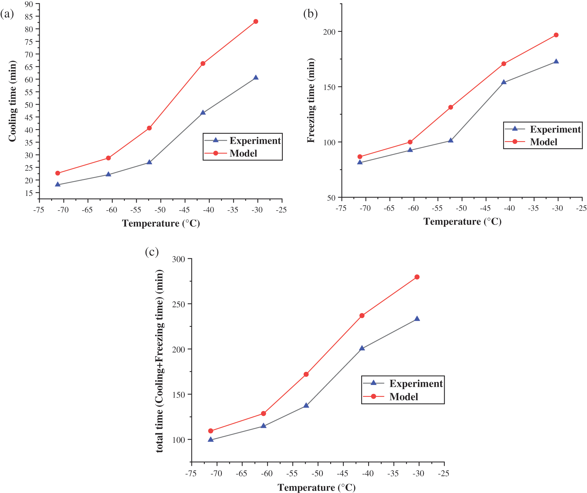
Figure 5: Comparison of heat transfer model and experiment in (a) cooling time, (b) freezing time and (c) total (cooling+freezing) time

4.3 Pipe Freezing Plugging Time Prediction

Based on the consistency between the heat transfer model and the experimental results, the model can be used to predict the time required for the freezing and plugging at different refrigeration temperatures when water is used as the plugging agent at an initial temperature of 25°C in the gas transmission pipeline. It provides a reference for predicting whether the plugging in the pipe is reached during the freezing and plugging. The calculation and prediction results are shown in Fig. 6. It can be seen that the freezing and plugging time of the pipe raises as the increasing of the pipe diameter and shortens with the decrease of the refrigeration temperature. When the refrigeration temperature is –30°C to –70°C, reducing the refrigeration temperature can significantly shorten the freezing and plugging time. When the refrigeration temperature is –70°C to –100°C, reducing the refrigeration temperature has little effect on the freezing and plugging time.

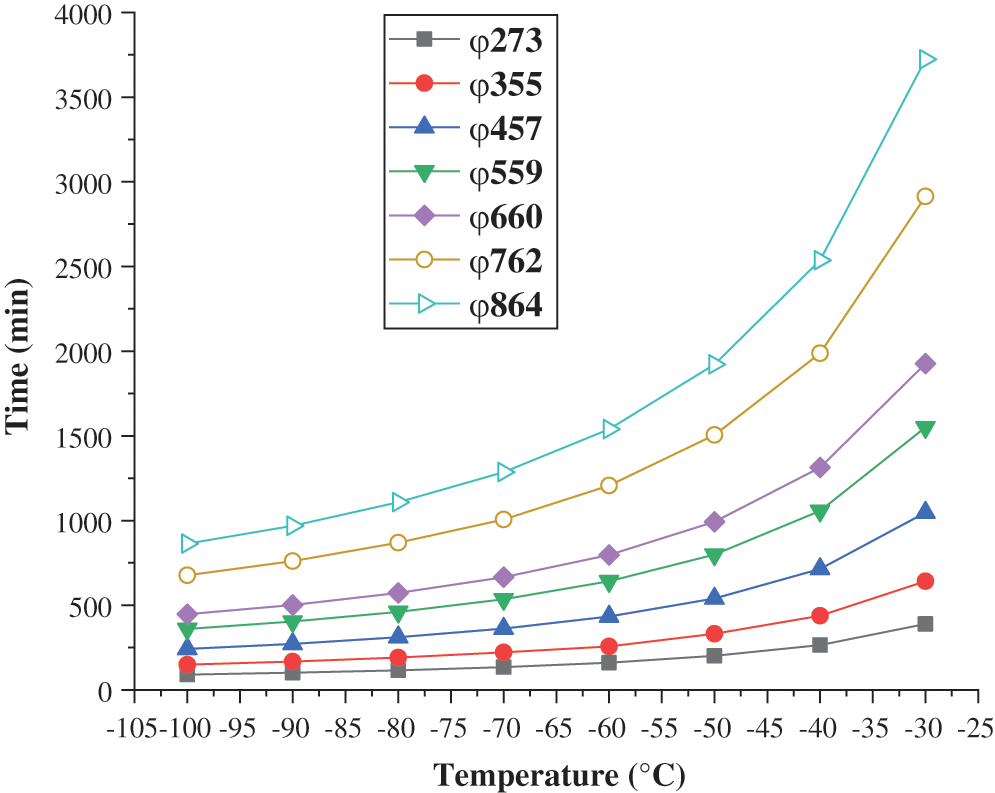
Figure 6: Prediction of freezing plugging time for pipes of different diameters

5  Conclusion

The main conclusions of this article are as follows:

(1) A heat transfer model that can be used to predict the transient temperature field and the position of the phase interface of the plugging agent in the pipeline during freezing and plugging of gas pipelines has been established.

(2) The heat transfer model was verified by a self-designed freezing and plugging experiment with water as a plugging agent. The results showed that the average error is 17.18%. And the greater the heat transfer temperature difference, the smaller the error is. The established heat transfer model is greatly consistent with the experiment.

(3) The heat transfer model is used to predict the time needed for freezing and plugging of gas pipelines with different diameters under different heat transfer conditions when water is used as the plugging agent, which provides a reference for whether the plugging conditions are achieved during the pipe’s freezing and plugging.

Acknowledgement: I gratefully acknowledge the guide of my teacher.

Funding Statement: The authors received no specific funding for this study.

Conflicts of Interest: The authors declare that they have no conflicts of interest to report regarding the present study.

References

 1.  Mokhatab, S., Poe, W. A. (2012). Handbook of natural gas transmission and processing. UK: Gulf Professional Publishing. [Google Scholar]

 2.  Ming, M., Hong, Z., Xin, S., Kun, L. (2014). The current development status and prospect of oil and gas pipeline plugging and emergency repair technology. China Petroleum Machinery, 42(6), 109–112. DOI 10.3969/j.issn.1001-4578.2014.06.026. [Google Scholar] [CrossRef]

 3.  Farrag, K. (2013). Selection of pipe repair methods. DOT Project No.: 359. USA: Office of Pipeline Safety. [Google Scholar]

 4.  Zhang, S., Li, Y., Ma, Y. M. (2009). Intelligent plugging techniques in high-pressure pipeline. Oil & Gas Storage and Transportation, 28(6), 59–61. [Google Scholar]

 5.  Song, Z., Liu, Z., Zhang, J., Chen, N., Zhou, L. et al. (2017). Technique of plugging with pressure applied in Ansai Oilfield pipeline maintenance. Petroleum Engineering Construction, 17(3), 17–19. DOI 10.3969/j.issn.1001-2206.2017.03.017. [Google Scholar] [CrossRef]

 6.  Chen, R., Yang, L. B., Xu, X. G. (2012). Troubleshooting of disc plugging device in rush repair of pipeline. Oil & Gas Storage and Transportation, 12(6), 16–19. DOI 10.6047/j.issn.1000-8241.2012.06.016. [Google Scholar] [CrossRef]

 7.  Cheng, S., Zhu, Y. (2016). Finite element analysis of online replacement of plugging capsule for long distance pipeline of refined oil. Journal of Xi’an Technological University, 16(6), 4–8. DOI 10.16185/j.jxatu.edu.cn.2016.06.004. [Google Scholar] [CrossRef]

 8.  Bishop, C. W. (1977). Pipefreezing-latest maintenance “tool” for pipeline engineers. Pipes and Pipelines International, 12(4), 16–40. [Google Scholar]

 9.  Bowen, R. J., Keary, A. C., Syngellakis, S. (1996). Pipe freezing operations offshore–some safety considerations. Proceedings of the international Conference on Offshore Mechanics and Arctic Engineering, pp. 511–516. USA. [Google Scholar]

10. Burton, M. J., Bowen, R. J. (1989). Effect of convection on plug formation during cryogenic pipe freezing. Chemical Engineering Research & Design, 67(2), 121–126. DOI 10.1016/B978-0-408-01259-1.50073-5. [Google Scholar] [CrossRef]

11. Keary, A. C. (1997). A numerical study of solidification and natural convection during cryogenic pipe freezing (Ph.D. Thesis). University of Southampton, UK. [Google Scholar]

12. Bueno, S. I. O., Murray, P. B. (2000). Freezing technique applied to an offshore pipeline at campos basin in Brazil. International Pipeline Conference, vol. 40252, pp. V002T07A007. USA, American Society of Mechanical Engineers. [Google Scholar]

13. Liang, Z., Lan, H., Li, L., Deng, X. (2010). Partial freeze sealing techniques for small-diameter natural gas pipelines. Natural Gas Industry, 24(9), 24–27. DOI 10.3787/j.issn.1000-0976.2010.09.018. [Google Scholar] [CrossRef]

14. Wang, X., Han, D., Chen, J., Li, H., Zhou, Y. (2012). Gas condensate pipe freezing blocking technology research and application. Petrochemical Industry Application, 12(3), 8–12. DOI 10.3969/j.issn.1673-5285.2012.03.015. [Google Scholar] [CrossRef]

15. Perkins H. C.Jr., Leppert G. (1964). Local heat-transfer coefficients on a uniformly heated cylinder. International Journal of Heat and Mass Transfer, 7(2), 143–158. DOI 10.1016/0017-9310(64)90079-1. [Google Scholar] [CrossRef]

16. Doktorov, E. V., Leble, S. B. (2007). A dressing method in mathematical physics, vol. 28. GER: Springer Science & Business Media. [Google Scholar]

17. Ã–zisik, M. N., Özışık, M. N., Özısık, M. N. (1993). Heat conduction. USA: John Wiley & Sons. [Google Scholar]

18. Akyurt, M., Zaki, G., Habeebullah, B. (2002). Freezing phenomena in ice-water systems. Energy Conversion and Management, 43(14), 1773–1789. DOI 10.1016/S0196-8904(01)00129-7. [Google Scholar] [CrossRef]

19. Shen, D., Si, H., Xia, J., Li, S. (2019). A new model for the characterization of frozen soil and related latent heat effects for the improvement of ground freezing techniques and its experimental verification. Fluid Dynamics & Materials Processing, 15(1), 63–76. DOI 10.32604/fdmp.2019.04799. [Google Scholar] [CrossRef]

20. Jeong, G. H., Ahn, B. J., Seong, Y. S., Kim, K. S. (2002). Numerical analysis of phase change and natural convection phenomena during pipe freezing process. ASME Pressure Vessels and Piping Conference, pp. 145–149. USA. [Google Scholar]

21. Kriraa, M., Souhar, K., Achemlal, D., Yassine, Y. A., Farchi, A. (2020). Fluid flow and convective heat transfer in a water chemical condenser. Fluid Dynamics & Materials Processing, 16(2), 199–209. DOI 10.32604/fdmp.2020.07986. [Google Scholar] [CrossRef]

This work is licensed under a Creative Commons Attribution 4.0 International License, which permits unrestricted use, distribution, and reproduction in any medium, provided the original work is properly cited.