Fluid Dynamics & Materials Processing

DOI: 10.32604/fdmp.2022.018628

ARTICLE

Simulation of the Hydraulic Behavior of a Bionic-Structure Drip Irrigation Emitter

Tianyu Xu1, Yanru Su1, Zhouming Su1, Shuteng Zhi1, Ennan Zheng1,* and Chengcheng Yan2

1School of Hydraulic and Electric Power, Heilongjiang University, Harbin, 150080, China
2School of Traditional Chinese Medicine, Zhejiang Pharmaceutical College, Ningbo, 315503, China
*Corresponding Author: Ennan Zheng. Email: xty1115291208@163.com
Received: 06 August 2021; Accepted: 15 October 2021

1  Introduction

Drip irrigation emitter is the core component of the drip irrigation system. The flow channel of the drip irrigation emitter affects the hydraulic performance and energy dissipation efficiency [1,2]. The hydraulic performance of the flow channel is expressed by the flow index, which indicates the sensitivity of the flow rate of the drip irrigation emitter to the inlet pressure [3,4]. The energy dissipation efficiency of the flow channel is expressed by the energy dissipation coefficient, which indicates the intensity of flow turbulence in drip irrigation emitter [5]. The geometric parameters of the flow channel have a significant impact on the uniformity and efficiency of the drip irrigation system [6,7]. Excessive geometric parameters will cause the uniformity of irrigation to decrease, and small geometric parameters will reduce the energy dissipation efficiency [8,9]. Therefore, the research on the relationship between the geometric parameters and the hydraulic performance of flow channels has always been a hot topic in the field of water-saving irrigation [10,11].

Computational fluid dynamics (CFD) is a new method to study the flow mechanism of emitters, reduce the development cost of emitters and shorten the test period, which makes up for the deficiency of the experiment to a certain extent [12,13]. Yuan et al. [14] used the CFD method to optimize the structure of the divided-flow drip irrigation emitter to obtain the functional relationship between anti-blocking performance and geometric parameters. Guo et al. [15] designed a two-way opposed flow channel and applied CFD to analyze the relationship between flow rate and working pressure. In order to improve the hydraulic performance and energy dissipation efficiency, many scholars had put forward many new design concepts and structural types of drip irrigation emitters [16,17]. The fractal flow channel designed on the basis of fractal theory can effectively reduce the flow index [18]. The triangle circulation flow channel can increase fluid turbulence and improve the uniformity of outlet flow-through internal large and small triangles [19]. A two-way flow channel with the combination of “V” shape and “∧” shape can improve the energy dissipation efficiency by mixing forward and reverse flow [20]. Xing et al. [21] used the bionic principle to design the drip irrigation emitter with a perforated plate structure, which had good hydraulic performance, and the flow index was 0.47–0.51.

Many inventions were derived from the bionics of plant structure or form, and plant bionics had a very wide range of applications. Based on the pressure drop similarity between the drip irrigation emitter and the torus-margo bordered pit structure of the plant xylem, the pit drip irrigation emitter was designed [22,23]. The bionic structure drip irrigation emitter (BSDE) was taken as the research objectives, numerical simulation and tests used to obtain pressure, and flow rate in the flow channel, combined with multiple regression models to establish a mathematical equation for calculating the flow index. It can: (1) obtain the flow index and the energy dissipation coefficient of the BSDE, (2) analyze the influence of geometric parameters on the performance of the BSDE, (3) evaluate the prediction model and flow characteristics of the BSDE. The results will provide a reference for the new bionic structure drip irrigation emitters and offer a deeper understanding of channel design in the drip irrigation technology.

2  Materials and Methods

2.1 BSDE Structure Design

The torus-margo bordered pit structure in plant xylem tracheids had good depressurization stability (Fig. 1a). According to the structure similarity, the pit drip irrigation emitter (PDIE) was designed [23]. Later research found that the BSDE had better working performance than the PDIE. The structure of PDIE and BSDE were shown in Figs. 1b and 1c.

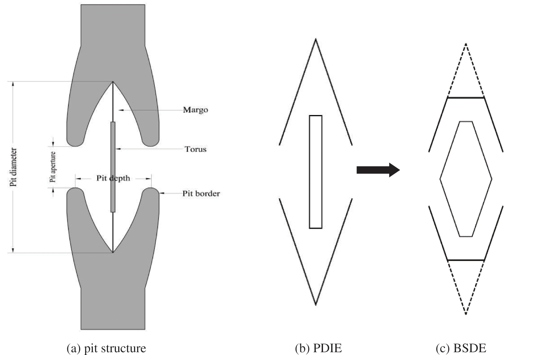
Figure 1: Schematic diagram of pit structure and two bionic models

2.2 Numerical Simulation and Test Model

2.2.1 Control Equation

The fluid flow relies on the steady-state conservation equations for mass and momentum in a fluid, which are given by [24,25]:

Continuity equation:

∂u∂x+∂v∂y+∂w∂z=0 (1)

Momentum equation:

{ ρ(u∂u∂x+v∂u∂y+w∂u∂z)=−∂P∂x+μ(∂2u∂x2+u∂2u∂y2+u∂2u∂z2)ρ(u∂v∂x+v∂v∂y+w∂v∂z)=−∂P∂y+μ(∂2v∂x2+u∂2v∂y2+u∂2v∂z2)ρ(u∂w∂x+v∂w∂y+w∂w∂z)=−∂P∂z+μ(∂2w∂x2+u∂2w∂y2+u∂2w∂z2)(2)

where u, v, w are the components of the velocity vector along the x, y, z-directions, respectively, ρ is the fluid density, P is the fluid pressure, µ is the dynamic viscosity.

In this study, a non-direct numerical simulation method was selected for analysis. The standard k–ε model had strong applicability to turbulent flow involved in BSDE model.

Its control equations are as follows:

∂(ρK)∂t+∂(ρkui)∂xi=∂∂xi[(μ+μtσk)∂k∂xj]+Gk+Gb−ρε−YM+Sk∂(ρε)∂t+∂(ρεui)∂xi=∂∂xj[(μ+μtσε)∂ε∂xj]+C1εεk(Gk+C3εGb)−C2ερε2k+Sε (3)

In the model, ε representing the turbulent dissipation rate was defined as:

ε=μρ(∂u′i∂xk)(∂u′j∂xk)¯ (4)

Gk representing the generation term of the turbulent energy k due to the average velocity gradient was defined as:

Gk=μt(∂ui∂xj+∂uj∂xi)∂ui∂xj (5)

Turbulent viscosity µt can be expressed as a function of k and ε as follows:

μt=ρCμk2ε (6)

where Gb was the generic term of the kinetic energy k caused by buoyancy, YM represented the contribution of pulsation expansion in compressible turbulence, C1Ɛ, C2Ɛ and C3Ɛ were the empirical constant, σk and σƐ were the Prandtl numbers corresponding to the kinetic energy k and the turbulent dissipation rate ε, respectively. Cμ was empirical constant, Sk and SƐ were user-defined source items, and the correlation values were: C1Ɛ = 1.44, C2Ɛ = 1.92, C3Ɛ = 1.44, σk = 1.0, σƐ = 1.3, Gb = 0, YM = 0, Cμ = 0.09, Sk = 0, SƐ = 0.

2.2.2 Structure and Geometric Parameters

The BSDE model was composed of inlet, flow channel and outlet (Fig. 2). The flow channel included pit aperture A(mm), pit depth B(mm), bottom height C(mm), left width E(mm) and right width D(mm) (Fig. 3a).

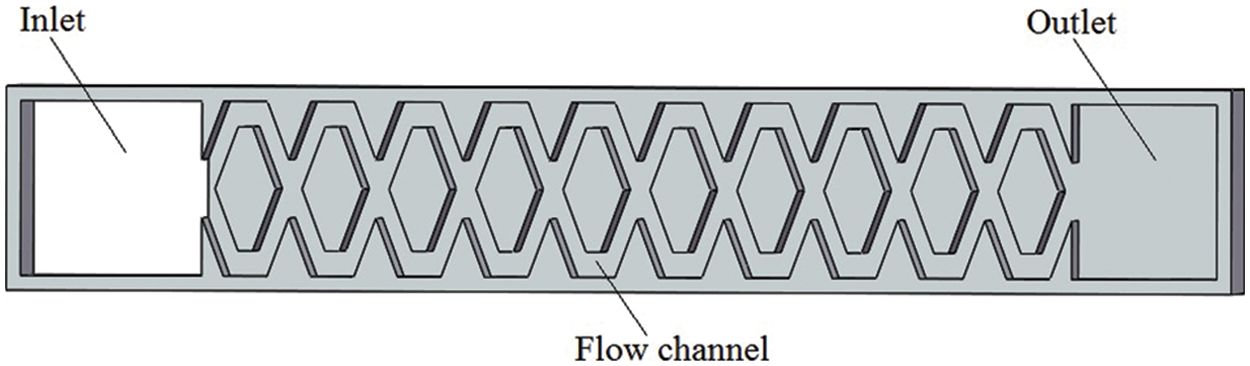
Figure 2: Schematic diagram of BSDE model

The value range of geometric parameters of the flow channel was as follows: A was 0.6 mm–1.0 mm, B was 1.0 mm–1.4 mm, C was 0.25 mm–0.45 mm, D was 0.12 mm–0.24 mm, E was 0.12 mm–0.24 mm. The pit diameter of the unit was 2.4 mm. The depth of BSDE model was 0.8 mm and the number of channel units was 10.

2.2.3 Meshing and Boundary Conditions

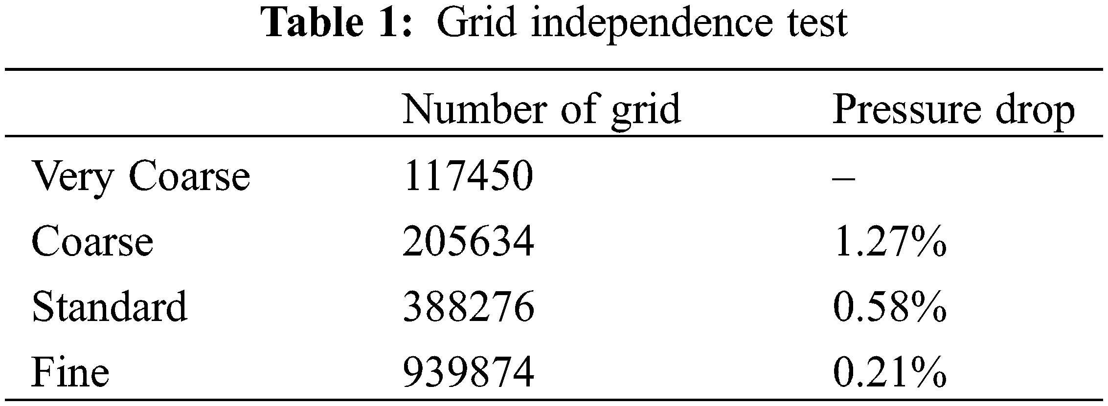
The BSDE model was built by SolidWorks software. The fluid domain was divided by unstructured grids of tetrahedron and hexahedron. Based on the prediction accuracy of the inlet and outlet pressure drop, the predicted pressure drop difference was less than 0.5% (Table 1), and it was considered that the number of grids had no effect on the numerical simulation results. The maximum element size was 3 × 10−5 m, the minimum element size was 1 × 10−5 m, and the total element number of the fluid domain was about 0.39 million. The grid of flow channels were shown in Fig. 3b.

Figure 3: Schematic diagram of the geometric parameters and meshing

The spatial discretization was based on the finite volume method. The second-order upwind scheme was adopted for the convection term. The coupling of velocity and pressure was solved by the SIMPLE algorithm, and the accuracy control standard was set to 10−5. The time step size was 0.02 s, Number of time step was 1000. The inlet of the flow channel was set to the pressure inlet, and the pressure values were set to 50, 75, 100, 125, 150, 175, 200, 225 and 250 kPa, respectively; the flow channel outlet was set to the outflow boundary. The no-slip condition was applied to the wall faces of the flow channel. The computing hardware platform was the five PowerCube-S01 cloud cubes high-performance parallel computers, and the ANSYS FLUENT 17.1 calculation software was used.

2.2.4 Construction of Test Model

The test rigs were 5 sets of test models. A pressure level set of tests was designed to each time 25 kPa increase within the pressure range of 50–250 kPa. Each test lasts 15 minutes, and 3 times of test measurements were done under each pressure level to take the average values. The BSDE models were made of plexiglass. An EM-G32S-X32 high-precision engraving machine with a manufacturing precision of 0.01 mm was used, and a repeating positioning accuracy was 0.005 mm. The physical picture of the plexiglass test model was shown in Fig. 4.

Figure 4: Prototype of BSDE model

2.3 Orthogonal Experiment Scheme

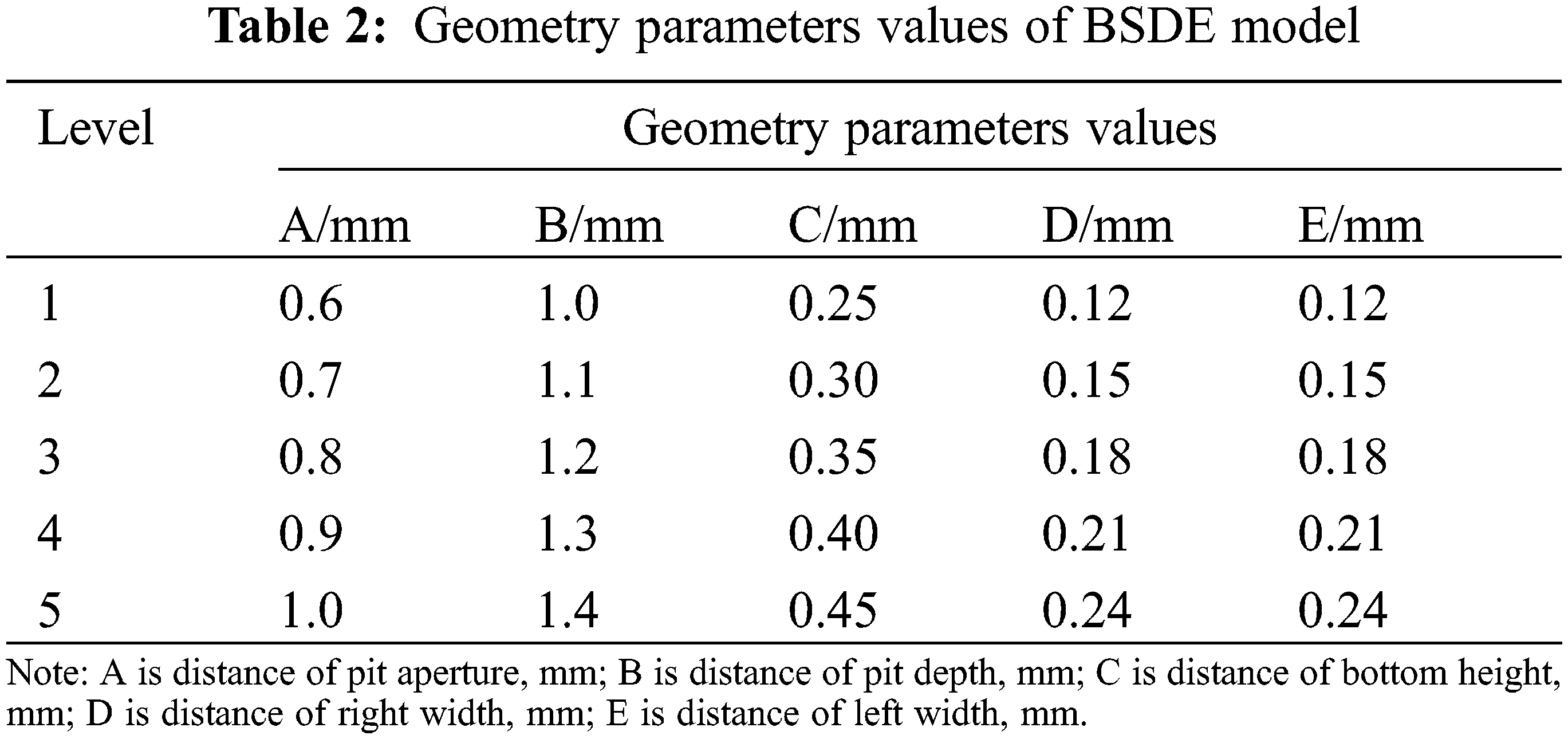
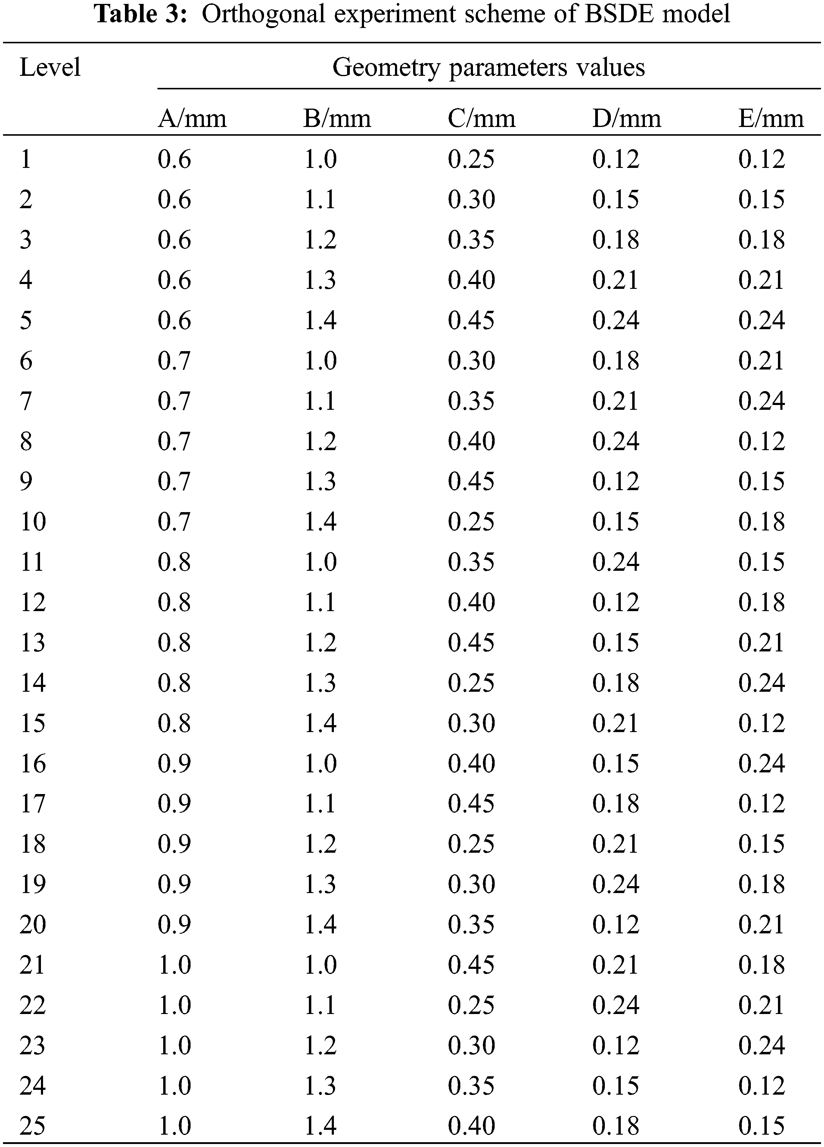
The geometric parameters of BSDE have adopted five factors and five levels (Table 2) and were designed according to the orthogonal experimental design table L25(56). The structure parameters values were shown in Table 3.

2.4 Calculation Method of Energy Dissipation Efficiency, Flow Index and Relative Error

The model can analyze the fluid flow in BSDE (Fig. 5) by the energy conservation law (Bernoulli equation). The flow between arbitrary sections satisfies the Bernoulli equation, which was written in sections from the inlet to the exit sections Z1, Z2, Zn as:

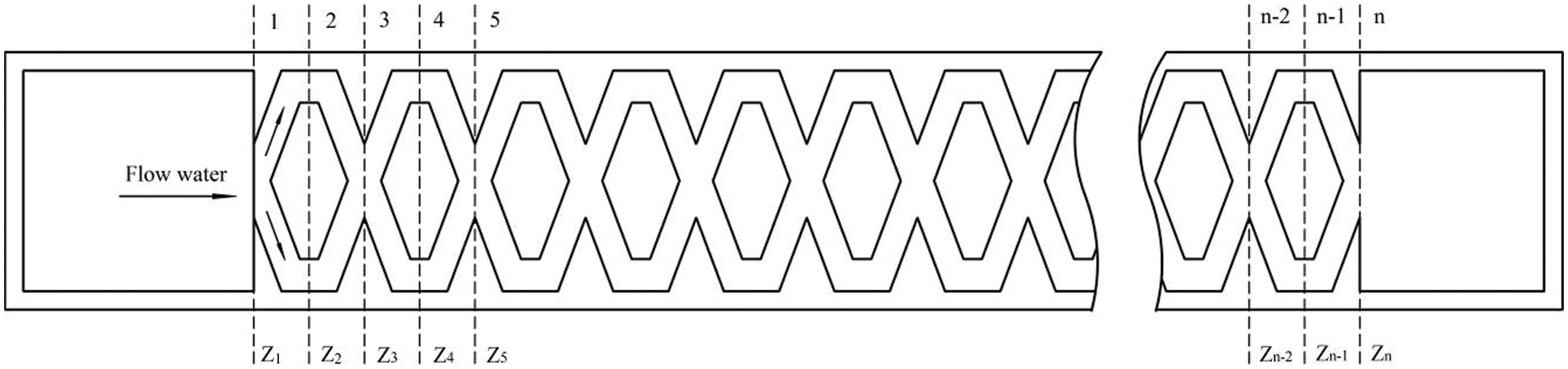
Figure 5: Schematic diagram of flow mechanism in BSDE model

P1ρg+V122g+z1=P2ρg+V222g+z2+ξ1V222g+λl1V228DgP2ρg+V222g+z1=P3ρg+V322g+z3+ξ2v322g+λl2V328Dg.............Pn−1ρg+Vn−122g+zn−1=Pnρg+Vn22g+zn+ξn−1Vn22g+λln−1Vn28Dg(7)

where Pn and Vn were the average pressure and flow velocity at section n, ρ was fluid density, g was the acceleration of gravity, zn was the position head of water at the section, ξn−1 was the local loss coefficient of section n−1 to section n, λ was the friction factor of head loss, ln−1 was the length between two adjacent sections. D was the hydraulic radius of the rectangular section flow channel. And a and b were the width and depth of the flow channel section, the expression of D was:

D=Aχ=ab2(a+b) (8)

Add the two sides of the equations of Eq. (7) in order:

P1−Pnρg=zn−z1+ξ1V222g+ξ2V322g+⋅⋅⋅+ξn−1Vn22g+λLVn28Dg (9)

where l1 + l2 + l3 + ··· + ln-1 = L, L was the total length of the flow channel. Positioning head due to the horizontal flow path, so Z1 = Z2 = Z3 = ··· = Zn.

Known by the continuity equation:

V1A1=V2A2=V3A3=⋅⋅⋅=VnAn (10)

In Eq. (10), Ai(i=1,2…,n) was the flow area at the corresponding section, substituting Eq. (10) into Eq. (9) give:

ΔPρg=[λ(A1An)2L4D+∑i=1n−1ξi(A1Ai+1)2]V122g (11)

where

ξ=[λ(A1An)2L4D+∑i=1n−1(A1Ai+1)2ξi] (12)

Eq. (11) was simplified to:

ΔPρg=ξV122g (13)

Expressed as:

ξ=2V12⋅ΔPρ (14a)

Expressed by flow rate:

ξ=2a2b2q2⋅ΔPρ (14b)

In Eqs. (14a) and (14b), ξ was the flow channel energy dissipation coefficient (frictional head loss and local head loss), q was the average flow rate of the flow channel. Obviously, ξ reflected energy dissipation capacity of BSDE. The expression of q was:

q=kHx (15)

where k was the flow coefficient; H was the inlet pressure, kPa; x was the flow index.

The relative error equation was as follows:

ε=S(T)−ES(T)×100 (16)

where ε was the relative error; S was the simulation value, l/h; T was the test value, l/h; and E was the estimated value, l/h.

3  Result

3.1 Flow-Pressure Relationship and Flow Index of Flow Channel

The orthogonal experiment numerical simulation results were shown in Table 4. Formula (15) was used to fit the relationship between flow rate and pressure, the coefficient of determination was 0.9998-0.9999, and the regression equation had a good correlation. The flow index of different geometric parameters was between 0.4757–0.5067. The schemes 12 and 18 were taken as examples (Fig. 6), the root means square error between the fitted value and the experiment value was 0.0053 and 0.0090 L/h, which more accurately reflected the relationship between the pressure and flow rate of the BSDE.

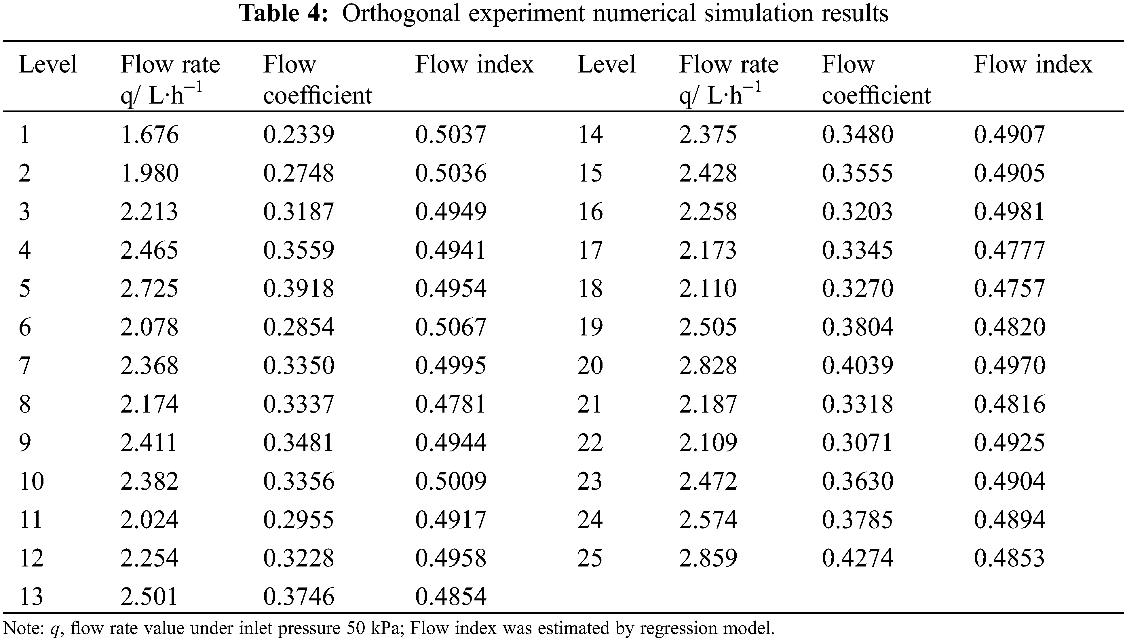
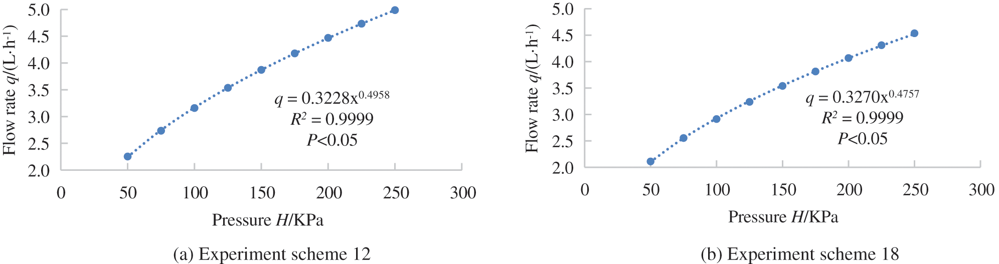
Figure 6: Relationship between flow rate and pressure for test schemes 12 and 18

3.2 Energy Dissipation Efficiency and Velocity Distribution

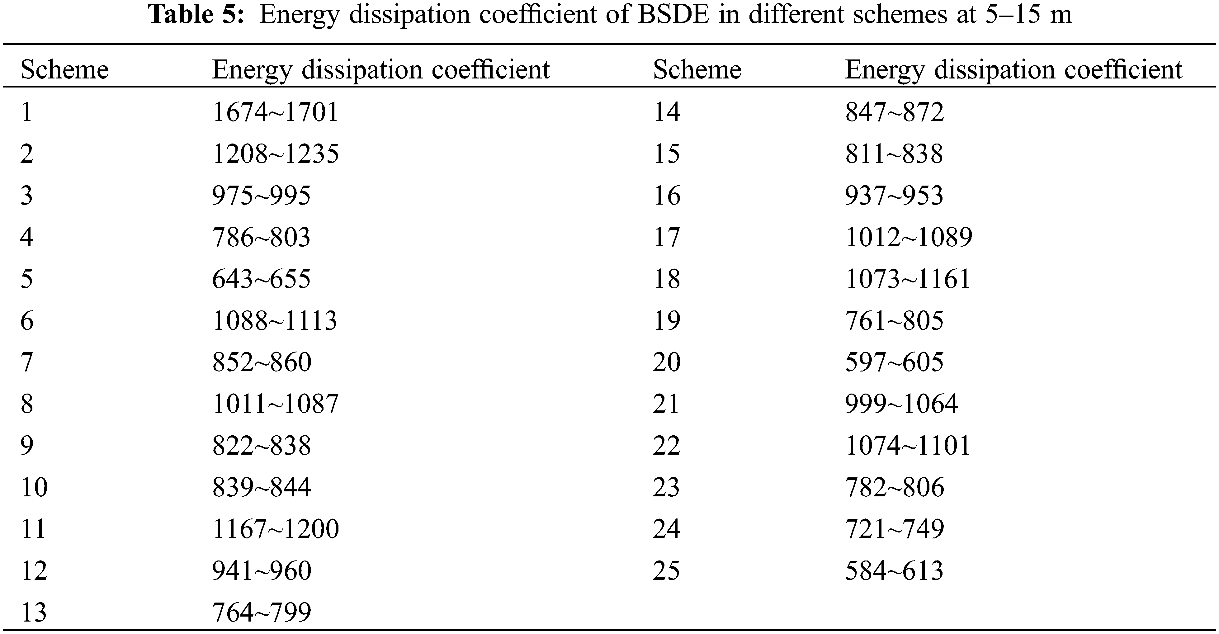
The energy dissipation efficiency of the BSDE was solved by the Bernoulli Eq. (14b). The results showed that the energy dissipation coefficient of the flow channel was 584–1701 at 5–15 m in the 25 experiment schemes (Table 5), which showed that the energy dissipation efficiency was obvious.

Taking scheme 1 (maximum energy dissipation coefficient) and scheme 25 (minimum energy dissipation coefficient) under 50 kpa pressure as the example. The fluid velocity at all points in the flow channel was not the absolute flow velocities in the BSDE (Fig. 7). However, the compared velocities within different locations in the flow channel were valid. By observing the velocity distribution of the two BSDE models, low-speed zone will be generated at the junction of the pit aperture, and high-speed zone will be generated at the left side of the tours. Experimental scheme 25 also produced obvious low-speed zones in the upper and lower corners. In the different low-speed zones of the BSDE model, a complete low-speed vortex was not observed, which had a good anti-blocking performance. The analysis of the flow velocity distribution and geometric parameters showed that the energy dissipation efficiency of the BSDE model was related to the flow rate and velocity distribution, the low-speed mixing of the junction area was conducive to energy dissipation.

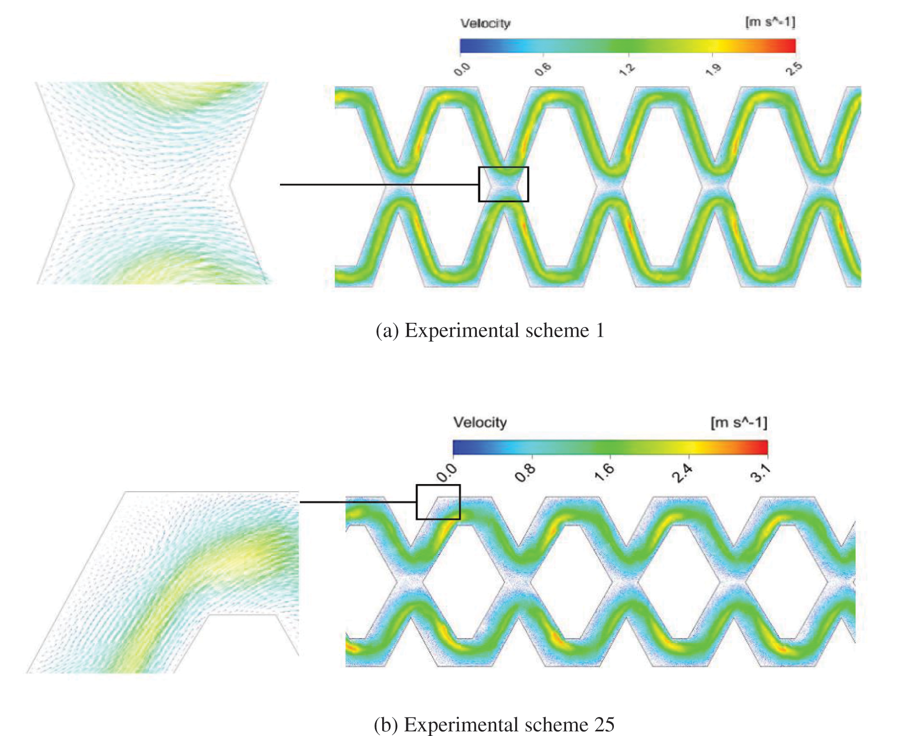
Figure 7: Relationship between flow rate and pressure for experimental schemes 1 and 25

3.3 Influencing Factors of Flow Index

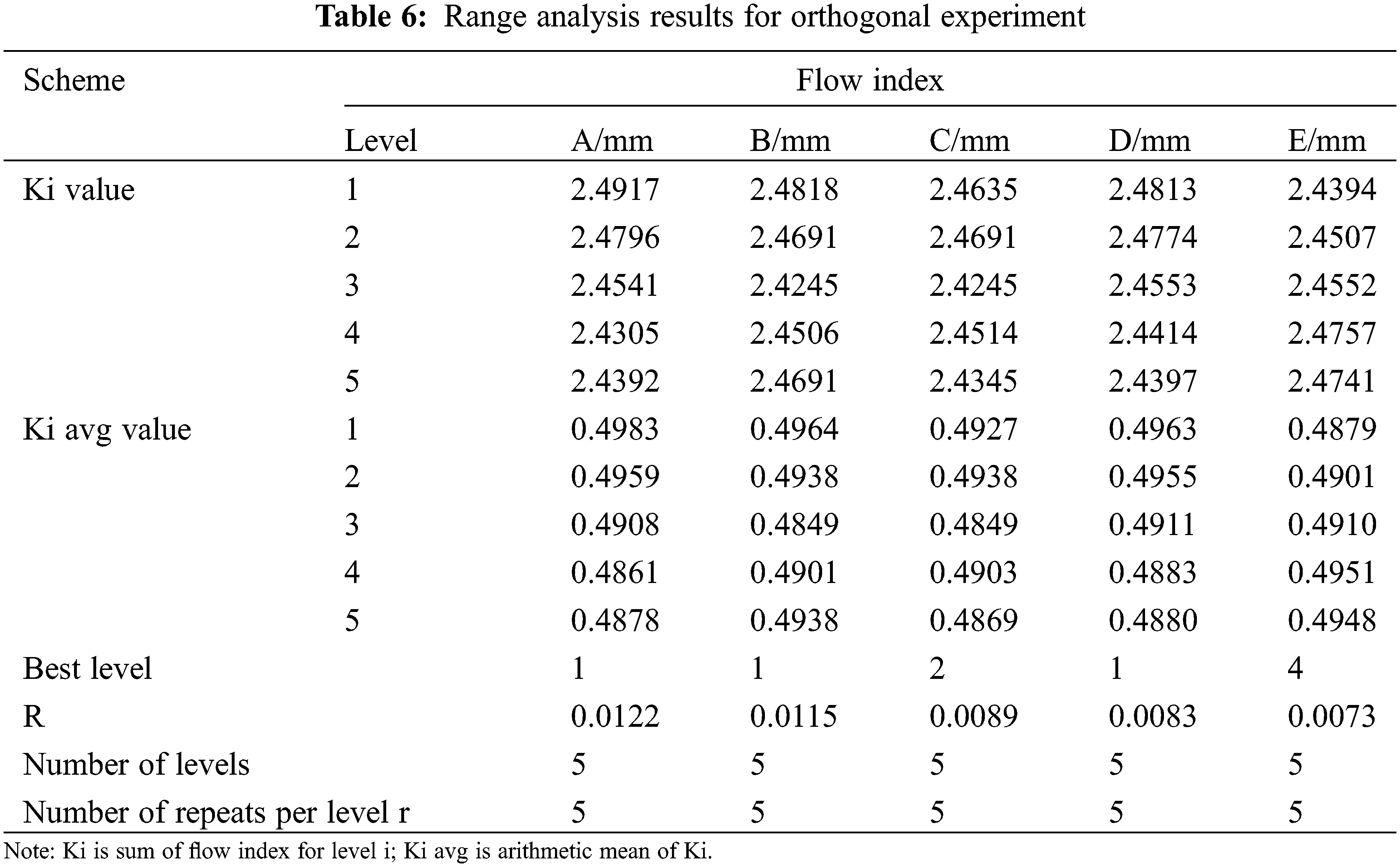
The range analysis of geometric parameters was implemented through the flow index values in Table 4. The range value showed that the order of the influence of each geometric parameter on the flow index was A > B > C > D > E. The optimal solution was A0.6B1.0C0.3D0.12E0.21 (Table 6).

Further analysis of the trend of the relationship between each parameter and the flow index (Fig. 8), it can be seen that the flow index decreased with the increase of A, B, C and D, and increased with the increase of E.

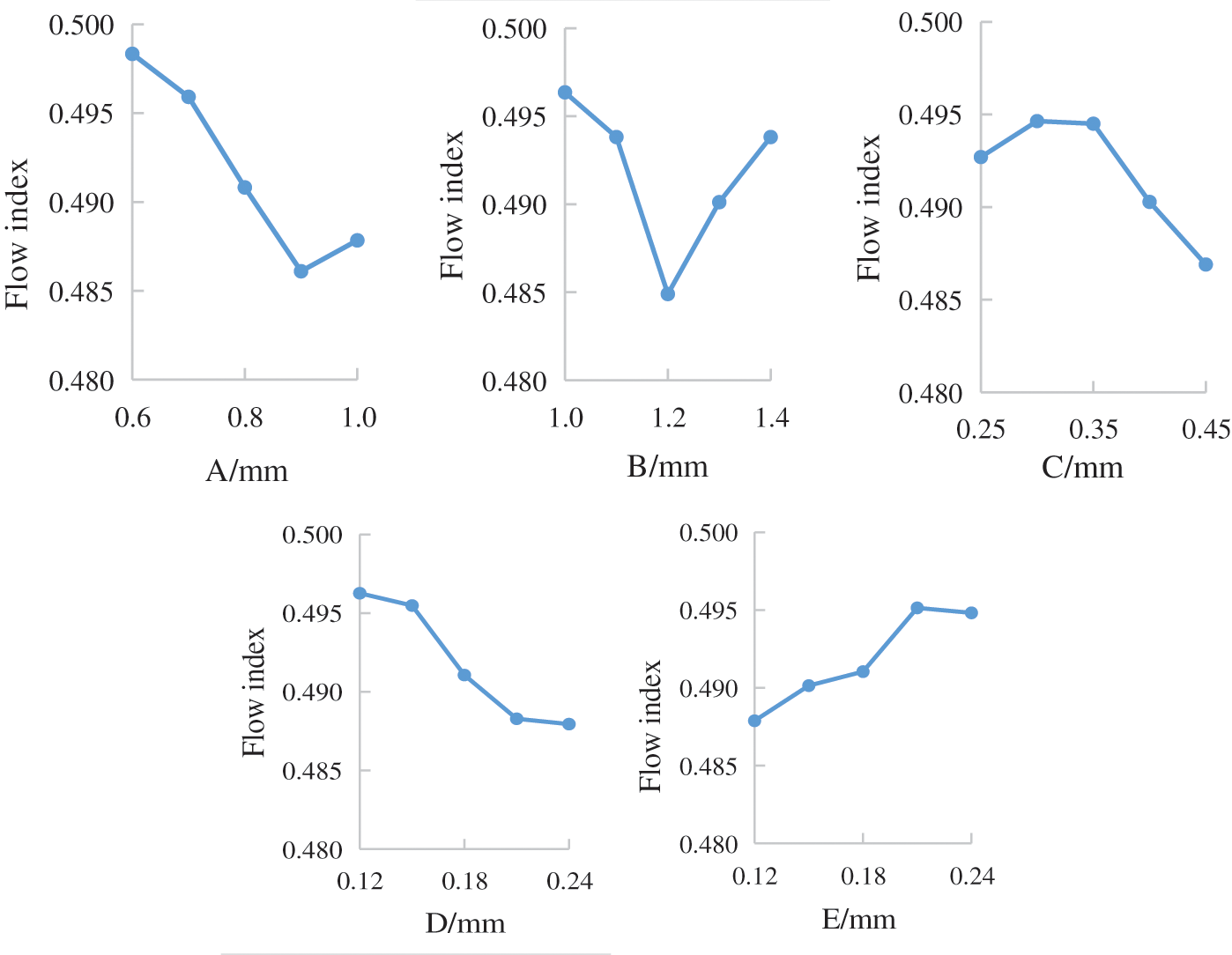
Figure 8: Effect of geometric parameter on flow index

3.4 Establishment and Verification of Flow Index Prediction Model

Based on the results of the orthogonal experiment, SPSS software was used to perform a multiple linear regression with a confidence level of 95%, and the regression model between the flow index and each parameter was calculated as:

x=0.5411−0.0308A−0.0088B−0.0319C−0.0795D+0.0629E (17)

The regression coefficient significance test F statistic value of this model was 6.997, the significance level Sig.= 0.001, the regression effect was significant, and the established regression equation was effective.

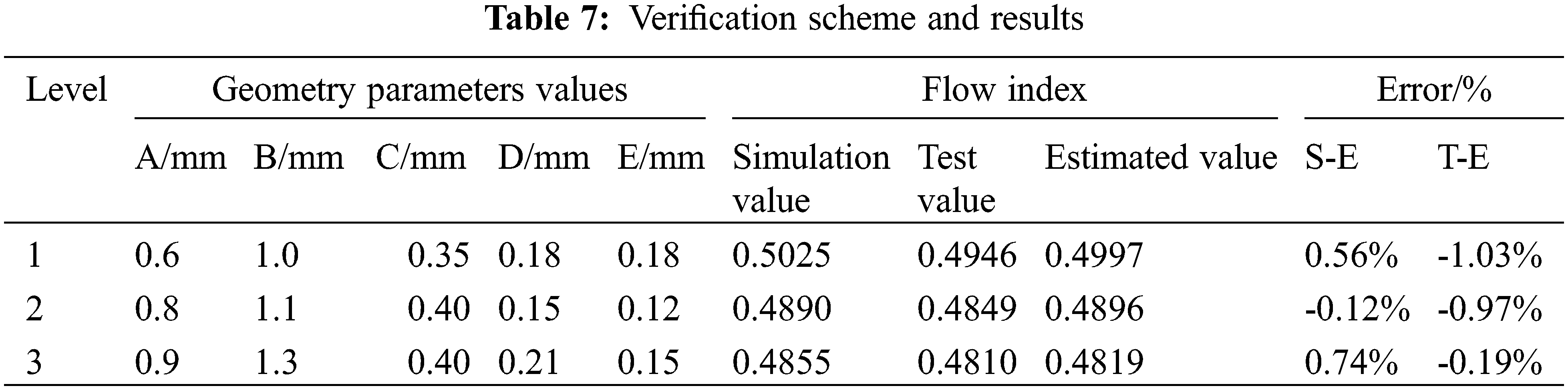
In order to further verify the reliability of the regression model, three groups of different flow channels were selected within the range of geometric parameters (Table 7), and the model samples were processed for testing and simulation. The estimated value was calculated by the formula (17) and the relative error was calculated by the formula (16). The calculation showed that the relative error of the flow index was −1.03% to 0.74%, which was less than 3%, indicating that the regression model of the formula (17) can accurately reflect the quantitative relationship between the flow index and the geometric parameters of the BSDE.

4  Conclusion

1.    The flow index of the BSDE was 0.4757–0.5067, indicating that its hydraulic performance was good. The energy dissipation coefficient under the pressure head of 5–15 m was 584–1701. Compared with the traditional unit flow channel structure, the energy loss effect was significantly improved, indicating that the structure of this type of drip irrigation emitter was reasonable.

2.    There was no low-speed vortex zone in the model flow channel, and the low-speed mixing of the junction area was conducive to energy dissipation. The results showed that the flow index decreased with the increase of A, B, C and D, and increased with the increase of E. The influence order of the geometric parameters on the flow index was A > B > C > D > E, The optimal solution was A0.6B1.0C0.3D0.12E0.21.

3.    The flow index prediction model was established, and the relative error among the test value, simulated value and estimated value was less than 3%, which proved the accuracy and reliability of the regression model.

Acknowledgement: Thank you to the co-operation and support of School of Hydraulic and Electric Power, Heilongjiang University, Harbin, 150080, China for this research.

Funding Statement: This work was supported by the Basic Scientific Research Fund of Heilongjiang Provincial Universities (2020-KYYWF-1042).

Conflicts of Interest: The authors declare that they have no conflicts of interest to report regarding the present study.

References

 1.  Madramootoo, C. A., Morrison, J. (2013). Advances and challenges with micro-irrigation. Irrigation and Drainage, 62(3), 255–261. DOI 10.1002/ird.1704. [Google Scholar] [CrossRef]

 2.  Al-Amoud, A. I., Mattar, M. A., Ateia, M. I. (2014). Impact of water temperature and structural parameters on the hydraulic labyrinthchannel emitter performance. Spanish Journal of Agricultural Research, 12(3), 580–593. DOI 10.5424/sjar/2014123-4990. [Google Scholar] [CrossRef]

 3.  Liu, C. J., Tang, D. B., Wang, L., Zhao, Z. (2016). Multi output optimization of the hydraulic performance for drip irrigation trapezoidal labyrinth channel of emitter. Arid Land Geography, 39(3), 600–606. DOI 10.13826/j.cnki.cn65-1103/x.2016.03.017. [Google Scholar] [CrossRef]

 4.  Souza, W. D. J., Sinobas, L. R., Sánchez, R., Botrel, T. A., Coelho, R. D. (2014). Prototype emitter for use in subsurface drip irrigation: Manufacturing, hydraulic evaluation and experimental analyses. Biosystems Engineering, 128(2), 41–51. DOI 10.1016/j.biosystemseng.2014.09.011. [Google Scholar] [CrossRef]

 5.  Ozekici, B., Sneed, R. E. (1991). Analysis of pressure losses in tortuous-path emitters, pp. 23–26. American Society of Agricultural Engineers (USAAlbuquerque, New Mexico. https://agris.fao.org/agris-search/search.do?recordID=US9511213. [Google Scholar]

 6.  Feng, J., Li, Y., Wang, W., Xue, S. (2018). Effect of optimization forms of flow path on emitter hydraulic and anti-clogging performance in drip irrigation system. Irrigation Science, 36(1), 37–47. DOI 10.1007/s00271-017-0561-9. [Google Scholar] [CrossRef]

 7.  Mohamed, A. M., Ahmed, I. A. (2017). Gene expression programming approach for modeling the hydraulic performance of labyrinth-channel emitters. Computers and Electronics in Agriculture, 142(2), 450–460. DOI 10.1016/j.compag.2017.09.029. [Google Scholar] [CrossRef]

 8.  Vekariya, P. B., Subbaiah, R., Mashru, H. H. (2011). Hydraulics of microtube emitters: A dimensional analysis approach. Irrigation Science, 29(4), 341–350. DOI 10.1007/s00271-010-0240-6. [Google Scholar] [CrossRef]

 9.  Wang, H. X., Zhang, X. Y., Niu, W. Q., Liu, M., Li, B. (2020). The effect of temperature on emitter clogging in low-pressure drip fertilization system. Journal of Irrigation and Drainage, 39(3), 63–71. DOI 10.13522/j.cnki.ggps.2019157. [Google Scholar] [CrossRef]

10. Hu, Y. X., Peng, J. Z., Yin, F., Liu, X. F., Li, N. (2020). Optimization and parameter analysis of trapezoidal labyrinth emitter channel based on MATLAB and COMSOL co-simulation. Transactions of the Chinese Society of Agricultural Engineering, 36(22), 158–164. DOI 10.11975/j.issn.1002-6819.2020.22.017. [Google Scholar] [CrossRef]

11. Philipova, N., Nikolov, N., Pichurov, G., Markov, D. (2009). Numerical simulation and a mathematical model of pressure losses depending on geometric parameters of drip emitter labyrinth channel. Comptes Rendus De l’Académie Bulgare Des Sciences: Sciences Mathématiques Et Naturelles, 62(7), 891–898. [Google Scholar]

12. Demir, V., Yurdem, H. U., Yazgi, A., Gunhan, T. U. (2019). Measurement and prediction of total friction losses in drip irrigation laterals with cylindrical integrated in-line drip emitters using CFD analysis method. Journal of Agricultural Sciences, 25(3), 354–366. DOI 10.15832/ankutbd.433830. [Google Scholar] [CrossRef]

13. Baghel, Y. K., Kumar, J., Patel, V. K. (2021). CFD Analysis of the flow characteristics of in-line drip emitter with different labyrinth channels. Journal of the Institution of Engineers (IndiaSeries A, 102(1), 111–119. DOI 10.1007/s40030-020-00499-5. [Google Scholar] [CrossRef]

14. Yuan, W. J., Wei, Z. Y., Chu, H. L., Ma, S. L. (2014). Optimal design and experiment for divided-flow emitter in drip irrigation. Transactions of the Chinese Society of Agricultural Engineering, 30(17), 117–124. DOI 10.3969/j.issn.1002-6819.2014.17.016. [Google Scholar] [CrossRef]

15. Guo, L., Bai, D., Wang, X. D., He, J., Zhou, W. et al. (2016). Hydraulic performance and energy dissipation effect of two-ways mixed flow emitter in drip irrigation. Transactions of the Chinese Society of Agricultural Engineering, 32(17), 77–82. DOI 10.11975/j.issn.1002-6819.2016.17.011. [Google Scholar] [CrossRef]

16. Wu, F., Dong, X. S., Wu, Y. B., Ma, D., Feng, X. F. (2017). Hydraulic properties of the flow in a gradual shrinking and sudden enlarging channel. Journal of North China University of Water Resources and Electric Power, 38(2), 61–67. DOI 10.3969/j.issn.1002-5634.2017.02.012. [Google Scholar] [CrossRef]

17. Yurdem, H., Demir, V., Mancuhan, A. (2015). Development of a simplified model for predicting the optimum lengths of drip irrigation laterals with coextruded cylindrical in-line emitters. Biosystems Engineering, 137(1), 22–35. DOI 10.1016/j.biosystemseng.2015.06.010. [Google Scholar] [CrossRef]

18. Li, Y., Yang, P., Ren, S. (2007). Effects of fractal flow part designing and its parameters on emitter hydraulic performance. Chinese Journal of Mechanical Engineering, 43(7), 109–114. DOI 10.3901/JME.2007.07.109. [Google Scholar] [CrossRef]

19. Guo, L., Bai, D., Cheng, P., Zhou, W. (2015). Optimization design of triangular labyrinth channel in drip irrigation emitter. Journal of Drainage and Irrigation Machinery Engineering, 33(7), 634–639. DOI 10.3969/j.issn.1674-8530.14.0164. [Google Scholar] [CrossRef]

20. Tian, J. Y., Bai, D., Ren, C. J., Wang, X. D. (2013). Analysis on hydraulic performance of bidirectional flow channel of drip irrigation emitter. Transactions of the Chinese Society of Agricultural Engineering, 29(20), 89–94. DOI 10.3969/j.issn.1002-6819.2013.20.013. [Google Scholar] [CrossRef]

21. Xing, S., Wang, Z., Zhang, J., Liu, N. N., Zhou, B. (2021). Simulation and verification of hydraulic performance and energy dissipation mechanism of perforated drip irrigation emitters. Water, 13(2), 171. DOI 10.3390/w13020171. [Google Scholar] [CrossRef]

22. Xu, T., Zhang, L. (2019). Hydraulic performance and energy dissipation effect of pit structure flow channel emitter. IFAC-PapersOnLine, 52(30), 143–148. DOI 10.1016/j.ifacol.2019.12.512. [Google Scholar] [CrossRef]

23. Xu, T., Zhang, L. (2020). Influence and analysis of structure design and optimization of a pit drip irrigation emitter on the performance. Irrigation and Drainage, 69(4), 633–645. DOI 10.1002/ird.2433. [Google Scholar] [CrossRef]

24. Ryad, C., Djamel, S., Adel, S., Smail, M. (2019). Numerical simulation of double diffusive mixed convection in a horizontal annulus with fifinned inner cylinder. Fluid Dynamics & Materials Processing, 15(2), 153–169. DOI 10.32604/fdmp.2019.04294. [Google Scholar] [CrossRef]

25. Basri, A. A., Zuber, M., Basri, E. I., Zakaria, M. S., Aziz, A. F. A. et al. (2021). Fluid-structure interaction in problems of patient specifific transcatheter aortic valve implantation with and without paravalvular leakage complication. Fluid Dynamics & Materials Processing, 17(3), 531–553. DOI 10.32604/fdmp.2021.010925. [Google Scholar] [CrossRef]

This work is licensed under a Creative Commons Attribution 4.0 International License, which permits unrestricted use, distribution, and reproduction in any medium, provided the original work is properly cited.