Fluid Dynamics & Materials Processing

DOI: 10.32604/fdmp.2022.019048

ARTICLE

Numerical Application of the Flamelet Model to Supersonic Turbulent Combustion

Yongkang Zheng1, Qinxue Jiang1,*, Hao Tian1, Youda Ye1 and Jingying Wang2

1China Aerodynamics Research and Development Center, Mianyang, 621000, China
2School of Energy and Power Engineering, Shandong University, Jinan, 250061, China
*Corresponding Author: Qinxue Jiang. Email: Jiangqinxue@cardc.cn
Received: 31 August 2021; Accepted: 15 November 2021

1  Introduction

Authors are encouraged to use the Microsoft Word template when preparing the final version of their manuscripts. In introduction, authors should provide a context or background for the study (that is, the nature of the problem and its significance). State the specific purpose or research objective of, or hypothesis tested by, the study or observation. Cite only directly pertinent references, and do not include data or conclusions from the work being reported. The theoretical performance of supersonic combustion for hypersonic vehicles has been discussed since the 1950s. However, because of the transitory residence time of inflow air in the combustor, many critical processes for supersonic combustion cannot be directly measured in experiments [1]. Moreover, supersonic flows are usually accompanied by a shock wave, which influences turbulent motion and flame development. The development of numerical simulation techniques for supersonic combustion flows has piqued the interest of researchers worldwide, especially for turbulent non-premixed combustion issues [2]. Therefore, computation is a useful supplement to physical understanding and algorithm design. After reviewing the development of numerical simulations for scramjet combustion, researchers have suggested that higher-order computational methods and more advanced turbulence-chemical interaction models, including flame-based methods, should be considered in practical scramjet systems. In addition, although some critical phenomena and supersonic combustion characteristics have been studied experimentally and numerically, there are still many uncertainties regarding the physical mechanisms of local extinction, reignition, and flame holding in real-world problems. Ladeinde [3] reviewed the history of scramjet combustion simulations by using various numerical models, revealing the flamelet method as an emerging model.

The traditional finite rate model treats turbulence and combustion as independent processes, ignoring the influence of turbulence fluctuations on the chemical reaction. However, the flamelet model assumes that the timescale of the chemical reaction is small enough that the thickness of the local instantaneous reaction layer is thinner than the Kolmogorov scale, and thus the chemical reaction in the reaction layer is unaffected by turbulence fluctuations. Previous studies [4] have shown that the combustion inside scramjets satisfies the flamelet assumption.

However, the flamelet model was originally designed for low-Mach-number flows and could not be directly extended to supersonic flows. Given the application of the flamelet model in supersonic combustion, Oevermann [5] proposed a novel strategy in which only the mean species mass fraction is calculated by the PDF integral of the flamelet library, and the mean temperature is solved implicitly by solving the energy equation. The flamelet model can be extended to more complex supersonic flows with this strategy, making it the standard method for flamelet model-based supersonic combustion simulations, including Reynolds-averaged Navier-Stokes simulations (RANS) and large eddy simulations (LES).

In this paper, the application of the flamelet model in supersonic flow is studied, and a representative experimental example is selected. The experiment is extended by using numerical simulations, and the numerical results of various properties are discussed in detail.

2  Numerical Methods

All numerical cases were simulated in a finite volume framework using an in-house code developed by the authors. Reynolds-averaged Navier–Stokes (RANS) simulations were used to solve the compressible governing equations as follows.

2.1 Governing Equations

Continuity equation:

∂ρ¯∂t+∂∂xj(ρ¯u~j)=0 (1)

Momentum equation:

∂∂t(ρ¯u~i) +  ∂∂xj(ρ¯u~iu~j+δijp¯)=∂∂xj(τ¯ij+τ¯ijt) (2)

Energy equation:

∂∂t(ρ¯E~) +  ∂∂xj(ρ¯H~u~j)=∂∂xj(λ∂T~∂xj+μtPrt∂h~∂xj+∑s=1ns⁡ρ¯Dsh~s∂Y~s∂xj+(μ+μtσk)∂k∂xj+(τ¯ij+τ¯ijt)u~j) (3)

Species continuity equation:

∂∂t(ρ¯Y~s)+∂∂xj(ρ¯Y~su~j)=∂∂xj((ρ¯Ds+μtSct)∂Y~s∂xj)+ω˙¯s (4)

The superscripts ‘−’ and ‘∼’ represent the Reynolds and Favre averages, respectively, and the specific variable symbols can be found in reference [6]. The viscous stress tensor is defined as:

τ¯ij=μ(∂u~i∂xj+∂u~j∂xi)−23δij(ρ¯k~+μ∂u~k∂xk) (5)

where δij is the Kronecker delta.

The state equation for the mixture gas is given as [7]:

p¯=RuT~∑s=1nsρ¯Y~sMs (6)

where Ru is the universal gas constant and Ms is the molecular weight of species s.

2.2 Turbulence Combustion Model

The flamelet model is used in this paper to evaluate the interactions between turbulence and combustion in supersonic flows because the mean chemical reaction rates ω˙¯s in Eq. (4) cannot be expressed directly. In theory, ω˙¯s are functions of the species mass fractions and temperature. The flamelet model is designed to directly model mean reaction scalar variables such as the species mass fractions and temperature rather than resolving the mean chemical source terms [8]. By introducing an additional variable called the mixture fraction, the simulations are decoupled from the inner flame structure and turbulent mixing process. The inner flame structure can be analyzed by solving the flamelet model equations. At the same time, the turbulent mixing process is introduced by the joint PDF of the mixture fraction and its dissipation rate. The flamelet equations are given as follows [8]:

ρ∂Ys∂τ=1LesρD(∂Z∂x1)2∂2Ys∂Z2+ρω˙s (7)

ρCp∂T∂τ=ρCpχ2∂2T∂Z2+∑s=1ns⁡ρhsω˙s+qR+∂p∂t (8)

By numerically solving Eqs. (7) and (8), the mass fraction and temperature are stored in a data list with the mixture fraction and scalar dissipation rate to generate the laminar flamelet library. The equivalent scalar dissipation rate χ is often used as the control variable of the turbulent flow field on the internal structure of the flamelet in the calculation because it changes with Z [9]. The laminar flamelet solutions Ys = Ys(Z, χst) and T = T(Z, χst) can be obtained by solving the flamelet governing equation. In this work, Flamemaster V4.0 [10] is used to solve flamelet Eqs. (7) and (8). Based on counterflow diffusion flamelet solutions, the software solves the equations by using an adaptive grid and a Newton iterative algorithm, which includes the detailed mechanism of the finite rate chemical reaction and the influence of variable Lewis numbers.

In general, the mixture fraction and scalar dissipation are physical quantities that vary with fluctuations of the flow field. Based on the instantaneous correlation of the mass fraction Ys, temperature T, mixture fraction Z, and equivalent scalar dissipation rate χst, the mean value of mass fraction and temperature can be obtained by integrating the joint probability density function (PDF) of the mixture fraction and scalar dissipation rate.

Y~s(xi)=∫01⁡∫0∞⁡Ys(Z,χst)P~(Z,χst;xi)dZdχst (9)

The joint PDF P~(Z,χst;xi) in Eq. (9) is obtained using the presumed PDF method [11]. Therefore, the transport equations of the first- and second-order moments of Z~ and Z~′′2 must also be solved [11]:

∂∂t(ρ¯Z~)+∂∂xj(ρ¯Z~u~j)=∂∂xj[(ρ¯D+μtSct)∂Z~∂xj] (10)

∂∂t(ρ¯Z˜''2)+∂∂xj(ρ¯Z˜''2u˜j)=∂∂xj[ (ρ¯D+μtSct)∂Z˜''2∂xj ]+2μtSct∂Z˜∂xj∂Z˜∂xj−ρ¯χ˜ (11)

In this work, the SST turbulence model [12] with compressibility correction is used, and an algebraic model of the mean scalar dissipation rate is established as follows:

χ˜=0.09cχωZ˜''2 (12)

The steady flamelet model (SF model) uses only the steady branch in the combustion solution of the flamelet equations, as shown in Fig. 1a. Because the curve has discontinuities between the critical extinction limit and the completely extinguished state, it cannot fully describe the intermediate state between steady-state combustion and the complete extinguished state. As a result, the steady flamelet model cannot capture local extinction and reignition in the flow field.

Figure 1: Maximum flame temperature, left: SF model, right: FPV model

Pierce [13] proposed the flamelet/progress variable model (FPV model) to address these problems. By introducing the progress variable C, the issue of discontinuity near the critical point is solved. Pierce [13] presented a complete numerical solution to the flamelet equations, which included three branches: the steady combustion branch, unsteady combustion branch, and completely extinguished branch. In the FPV model, the definition of the progress variable C is determined by the specific combustion problem, and different definitions of the progress variable are used for the chemical reaction processes of different fuels and oxidants. For the standard reaction model in general engineering problems, the progress variable must reflect the process of the whole chemical reaction and correspond to any flame state; thus, the mass fraction of the final product, rather than the intermediate production, is generally chosen as the progress variable. In this paper, only hydrogen fuel is studied, and thus the chemical reaction process is the hydrogen-oxygen reaction mechanism. Therefore, the mass fraction of water is selected as the progress variable C.

The S-shaped curve of the maximum flame temperature vs. the equivalent scalar dissipation rate can be obtained by solving the flamelet equations, as shown in Fig. 1b.

Fig. 1b shows that the maximum flame temperature gradually decreases with the steady combustion branch. An increase in χst enhances the nonequilibrium effect, improves mixing and diffusion between substances, and increases the reactant concentration. The reaction intensity, product concentration, and maximum flame temperature all decrease. As χst continues to increase toward the tipping point, the flame temperature remains at a local critical minimum; the flame completely extinguishes when χst is slightly above the tipping point. However, there is an apparent transition state between the complete combustion and completely extinguished states known as the unsteady combustion branch. Along this branch, the dissipation rate decreases as the flame temperature decreases, and the mixing equilibrium state is maintained at a lower reaction rate. In the completely extinguished state, the effect of chemical kinetics is negligible, and the chemical state is independent of the dissipation rate.

∂∂t(ρ¯C~)+∂∂xj(ρ¯C~u~j)=∂∂xj[(ρ¯D+μtSct)∂C~∂xj]+ω˙~C (13)

2.3 Discretization

In this paper, the compressible Navier–Stokes equations are discretized using the finite volume method based on a multiblock structured grid framework. A second-order MUSCL scheme with a minmod limiter is used to calculate the inviscid flux vector, and a second-order central difference scheme is used to calculate the viscous flux vector. The LDFSS flux splitting scheme [14] is also used. The time advance is evaluated by the implicit LUSGS method [15]. To satisfy the computational requirements, the Massage Passing Interface (MPI) is used for parallel computations to improve computing efficiency.

3  Code Validation

The German Aerospace Center (DLR) provided experimental schlieren diagrams of a supersonic combustor, flow field pressure distributions, and experimental velocity and temperature measurement results [16] for both cold flow mixing and combustion experiments. This is the most commonly used example for testing numerical calculation methods and combustion models in supersonic combustion simulations. The experiment was numerically simulated with calculation methods such as the RANS method [17], the mixed RANS/LES method [18], and the LES method [19].

3.1 Geometry and Flow Conditions

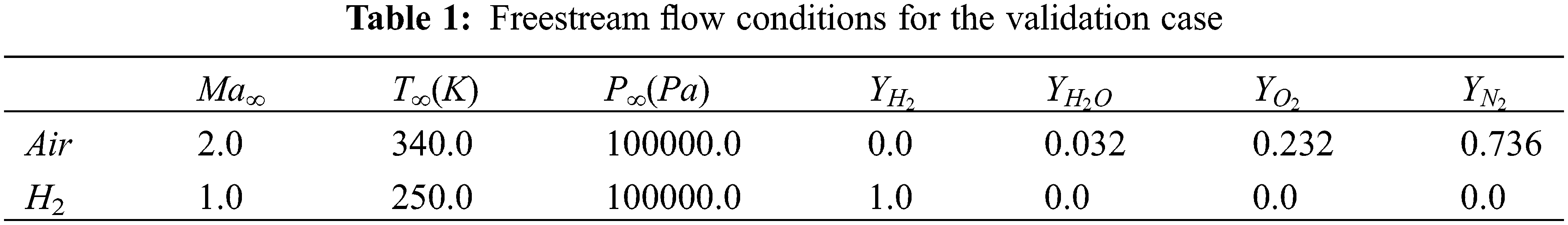
Schematic diagrams of the experimental device and the central strut are given in Fig. 2. A detailed description of the combustion chamber shape and structure have been previously introduced in the literature. The bottom of the strut is located at X = 62 mm, and 15 circular jet holes with diameters of 1 mm and spacings of 2.4 mm are evenly arranged along the spreading direction. Hydrogen is horizontally injected into the combustion chamber through the 15 holes. Table 1 shows the calculation dimension diagram and the calculation grid. The required width for the RANS method can be guaranteed by taking the area between the middle line of the two holes and the center of one of the holes. The spatial distribution of the calculated grid is shown in Fig. 3. There are approximately 2.11 million grids in total.

Figure 2: Schematic description of the experimental facility [16]

Figure 3: Topology of the medium grid for the DLR geometry

3.2 Grid Sensitivity Analysis

Previous studies have shown that the grid spacing in the normal direction of the wall is critical for obtaining reliable numerical simulation results. Based on previous numerical experience, the grid Reynolds number [20] is introduced to determine the height of the first grid:

ReΔ=ρ∞u∞Δμ∞ (14)

where ρ∞, u∞, μ∞ are the freestream density, velocity and viscosity, respectively, and Δ is the first grid scale in the wall-normal direction.

To ensure the reliability of the following calculation, the convergence of the grid spacing needs to be verified first. Based on the empirical grid setting strategy [21–23], three different grid spacing scales are adopted to represent the independence of the grid: coarse, medium, and fine. The detailed grid information and the distribution of the medium grid are shown in Table 2 and Fig. 3, respectively.

Two typical locations (X = 78 mm and X = 207 mm) were selected to investigate the distribution of the flow field variables calculated by the three types of grids. Fig. 3 shows the distribution of the flow velocity along the Y direction at these two locations. The numerical results for the three sets of grids are nearly identical in the upstream region. As the flow and combustion process develop in the downstream area, the medium and fine grids remain constant, while the coarse grid begins to diverge. This shows that the code used in this work is capable of ensuring grid independence. Considering the trade-off between computational cost and numerical precision, the medium grid is preferable. In the following section, the flow field analysis is carried out based on the numerical results of the medium grid.

A comparison between the experimental schlieren image and the density gradient distribution of the calculated results is shown in Fig. 4. The oblique shock wave formed at the leading edge of the strut and its reflection process between the shear layer and the upper and lower walls can clearly be seen in Fig. 4. The numerical flow field structure, including the Mach number distribution and the streamline distribution near the bottom of the strut, is shown in Fig. 5. Fig. 6 shows that, according to the experimental results, the combustion area of the flow field downstream of the strut can be divided into three regions based on the combustion mechanism: the induced zone, the transition zone, and the turbulent combustion zone. In the induction zone, there is a stable backflow at the trailing edge of the strut, leading to low-speed and high-temperature flow in the region. Following the injection of hydrogen into the region, the hydrogen combines with oxygen and successfully ignites. In the transition zone, a large-scale vortex structure forms due to the influence of the shear layer and the oblique shock wave acting on the shear layer. These vortex structures transfer the momentum of the outer low-temperature gas into the inner high-temperature gas through a momentum exchange mechanism. The subsonic gas in the combustion zone gradually accelerates and forms supersonic flow. In the turbulent combustion zone, the large-scale vortex structure upstream is constantly distorted and deformed by the stretching of the shear layer and gradually breaks into small-scale vortex structures, forming a stable turbulent diffusion combustion zone.

Figure 4: Velocity distribution, left: X = 78 mm, right: X = 125 mm

Figure 5: Density gradient distribution contours of the full configuration for DLR geometry

Figure 6: Mach contour distribution (left) and streamline distribution (right) of the DLR geometry

Three specific positions along the flow direction are selected for comparisons between the numerical results and the experimental data. Figs. 7 and 8 show the temperature and flow velocity and distributions. The ‘double peak’ structure of the temperature curve is clearly visible at X = 78 mm. The numerical results are consistent with the experimental data in Figs. 7 and 8.

Figure 7: Temperature distribution, left: X = 78 mm, middle: X = 125 mm, right: X = 233 mm

Figure 8: Velocity distribution, left: X = 78 mm, middle: X = 125 mm, right: X = 207 mm

4  Computational Details

In this paper, the numerical simulation of a slope injection with fuel-enhanced mixing by the streamwise vortex is studied. When supersonic air flows through the edge of the slope, it follows the incoming flow downstream and gradually develops into a pair of streamwise vortexes. A recirculation zone can be formed at the bottom of the slope, where the high enthalpy inlet flow slows down and increases the temperature, creating an ideal combustion environment. After injection, the fuel is rolled into the main flow area by the streamwise vortex and thoroughly mixed with oxygen for intense combustion. After the reflection of the upper wall, the oblique shock wave generated by the slope collides with the vortex structure in the main flow area of the combustion chamber, potentially causing the vortex to break up. At the same time, the reflected shock wave collides with the turbulent boundary layer of the lower wall, resulting in separation and the formation of new streamwise vortices.

4.1 Geometry and Flow Conditions

The numerical simulation is based on a supersonic combustion flow experiment with increased slope and cavity mixing conducted by Arail [24] at Osaka Prefectural University. During the wind tunnel experiment, slope and step diversion devices are arranged on the lower wall of the combustion chamber, and a cavity is installed on the upper wall. Two experimental states (with and without cavities) are observed to investigate the action mechanisms of the shock wave, boundary layer, and flow oscillation. Fig. 9 shows the combustion chamber and the slope device. Arai only observed the effects of the slope and the cavity on supersonic flow without performing relevant outflow and combustion experiments. In this paper, numerical simulations are used to extend this experimental research by adding a circular hydrogen hole with a diameter of 1 mm to investigate the slope and cavity of the combustion flow field. The grid distribution of the combustion chamber with a cavity is shown in Fig. 9. The cavity combustor has approximately 11 million grids, while the non-cavity combustor has approximately 9 million grids. An adiabatic wall is used to calculate the inflow parameters, which are listed in Table 3.

Figure 9: Schematic description of the experimental configuration and topology of the grid

4.2 Results and Discussions

After hydrogen fuel is injected into the combustion chamber along the flow direction from the bottom of the step, it is thoroughly mixed with the incoming air via the entrapment action of the streamwise vortex to form a stable turbulent combustion flow. In this section, the mixing and combustion characteristics of the ramp injection fuel scheme and the influence of the upper wall cavity on the flow are studied.

Fig. 10 shows a comparison between the calculated density gradient distribution at the axial center section of the two groups of shapes and the instantaneous schlieren diagram in the experiment. The wave structure in the combustion chamber can be clearly distinguished in the figure. In the experiment, the incoming air forms an oblique shock wave after compression at the leading edge of the slope, which interferes with the boundary layer at the upper wall and acts on the lower wall after reflection. The airflow is compressed again at the trailing edge of the ramp, forming a second oblique shock wave and reflecting at the upper wall of the middle section of the combustion chamber. When a square chamber is placed on the upper wall of the combustion chamber, the shear flow generated by the square chamber interferes with the first oblique shock wave, causing oscillations. The wave system for the square chamber has a slightly different shape than for the non-square chamber. After the airflow bypasses the slope and steps, a pair of reverse flow vortices form. After the upper wall reflects the front shock wave, it strikes the area where the vortexes flow, accelerating the rupture and amplifying the mixing effect. Because this paper only uses steady-state calculations and the time format has first-order accuracy, the process of flow oscillation near the square cavity cannot be captured. This can only be demonstrated by the time-averaged flow phenomenon and wave system structure in the flow field. The most significant difference between the numerical results and the experimental schlieren chart is that the influence of the hydrogen jet on the trailing edge of the step is considered. From Fig. 10, it is clear that the hydrogen gas emitted at the speed of sound and the incoming gas flowing at the external supersonic velocity shear, as well as the process of momentum displacement out of the shear layer by the small vortex structure formed by the shear, improve flow mixing. The calculation results shows that the shear layer blocks the shock wave reflected from the upper wall; thus, it has little effect on the combustion process in the central zone. This section uses the square cavity calculation results from the combustion chamber shape analysis to study the flow characteristics of the slope injection combustion scheme.

Figure 10: Density gradient distribution contours of the full configuration

Fig. 11 shows cloud maps of the Mach number and vorticity distributions for the strike-center section as well as different stations in the flow direction, representing the shock wave structure and vortex distribution of the flow field in the combustion chamber. The seven sections of the flow direction are located at X = −5, 2.5, 10, 28, 50, 70, and 95 mm. After the incoming air passes through the step, an expansion wave forms. After injecting hydrogen, an induction zone forms in the low-speed area at the back edge of the step. There is a stable backflow in this area, with a low-speed and high-temperature flow. There is a velocity difference between the wake of the hydrogen jet and the free flow, resulting in the formation of a shear layer; the flow forms the main flow area between the shear layer and the lower wall. When the incoming air bypasses the slope and steps, a pair of counterrotating streamwise vortices forms. As the vortex moves downstream in the main flow area, hydrogen is constantly picked up and diffuses to the surroundings, causing the hydrogen fuel and the surrounding air to quickly mix. At the same time, vortex flow in the shear layer interacts with the turbulent boundary layer near the sidewall region, resulting in a high-temperature, low-speed environment that increases the residence time of both fuel and air and enhances the turbulent combustion process. As shown in Fig. 11, the vorticity value and vorticity intensity are highest behind the steps. The impact on fuel mixing is also the most obvious here. As it moves downstream, the large-scale vortex is gradually broken down into small structures under the influence of shear layer flow and turbulent combustion. Energy is transferred downward in stages. As a result, the vortex decreases along the flow direction, and its intensity continuously decreases.

Figure 11: Mach contour distribution and vorticity contour distribution

Fig. 12 shows the pressure distribution of the lower wall surface and the three-dimensional streamline distribution behind the step. Due to the downward expansion of the slope, a low-pressure expansion area forms near the lower wall surface. Due to the positive pressure gradient, the flow bends to the slope and the step. As shown by the streamline distribution in the figure, the vortex can transfer hydrogen fuel ejected from the center behind the steps to both sides. As it travels downstream, the hydrogen combines with oxygen, resulting in violent combustion. Fig. 13 shows the distribution of the hydrogen and water on the U = −1.0 m/s isosurface behind the steps. Fig. 11 shows that the hydrogen jet column expands rapidly due to the action of the vortices. In addition, chemical reactions with oxygen are considerably reduced. Fig. 13 shows that chemical reactions in the reflux area are sufficient, and the water that is generated is evenly distributed in the reflux area. Almost every area was entirely chemically reacted.

Figure 12: Pressure contour distribution for the bottom wall with streamline distribution

Figure 13: U = −1 m/s contour surface with H2 and H2O

The temperature distributions and superposition of sound velocity lines at the spanning center cross-section and various flow direction cross-sections are shown in Fig. 14. Most areas of the supersonic combustor have supersonic flow, with only the backflow zone behind the step, the inner cavity, and the wall area behind the step having subsonic flow. This indicates that the primary reaction zone is the supersonic combustion mode. The subsonic combustion mode is mainly distributed in the backflow zone and near the wall area behind the step. The high-temperature region in the mainstream zone is concentrated within the shear layer, and the high-temperature zone is initially formed under the jet wake. Due to the entrainment of the vortex, hydrogen and oxygen quickly mix inside the vortex and fully react, forming a stable high-temperature combustion environment. As a result of the turbulent boundary layer, a stable combustion phenomenon forms in the bottom wall boundary layer, indicating that turbulence promotes combustion.

Figure 14: Temperature contour distribution

The density gradient distribution in Fig. 10 shows that, due to the blocking effect of the shear layer on the reflected shock wave and the expansion wave system structure in the flow field space, the wave system effect and the shear effect generated by the square cavity have little effect on the turbulent combustion process in the mainstream area. Figs. 15 and 16 show the mass fraction distributions of H2O and OH, respectively, in the central section with or without a square cavity. The distributions of intermediate OH and water in the two configurations is nearly identical. This shows that the square cavity has no effect on the intermediate or final stages of combustion.

Figure 15: H2O contour distribution, left: with cavity, right: without cavity

Figure 16: OH contour distribution, left: with cavity, right: without cavity

5  Conclusion

In the current study, the influence of the flamelet/progress variable model on the flow field prediction of a scramjet is numerically analyzed. The standard SST turbulence model is used for turbulent transport, and the flamelet model is used for chemical reactions. The main conclusions are summarized as follows. A pair of streamwise vortices form in opposite directions after the airflow bypasses the slope and the step. The shock waves generated by the front edge of the step are reflected by the upper wall and collide with the vortex region, accelerating the vortex rupture and amplifying the mixing effect. Unfortunately, the steady-state method used in this paper does not capture the oscillating flow at the inlet of the square cavity. However, when the influence of the wave structure in the flow field is considered, the influence of the square cavity on flow and turbulent combustion is minimal.

Acknowledgement: The first author, Yongkang Zheng acknowledges the National Laboratory for Computational Fluid Dynamics for the computational resources and technical support.

Funding Statement: This work was supported by the National Natural Science Foundation of China (No. 12002193), and the Shandong Provincial Natural Science Foundation, China (No. ZR2019QA018).

Conflicts of Interest: The authors declare that they have no conflicts of interest to report regarding the present study.

References

 1.  Pecnik, R. (2012). Reynolds-averaged Navier-stokes simulations of the HyShot II scramjet. AIAA Journal, 50(8), 1717–1732. DOI 10.2514/1.J051473. [Google Scholar] [CrossRef]

 2.  Baurle, R. A. (2014). Modelling of high speed reacting flows: Established practices and future challenges. 42nd AIAA Aerospace Sciences Meeting and Exhibit, Reno, Nevada. AIAA Paper, 2004–2267. DOI 10.2514/6.2004-267. [Google Scholar] [CrossRef]

 3.  Ladeinde, F. (2009). A critical review of scramjet combustion simulation. 47th AIAA Aerospace Sciences Meeting Including the New Horizons Forum and Aerospace Exposition, Orlando, Florida. AIAA Paper, 2009–2127. DOI 10.2514/MASM09. [Google Scholar] [CrossRef]

 4.  Gao, Z. X., Lee, C. H. (2010). A numerical study of turbulent combustion characteristics in a combustion chamber of a scramjet engine. Science China Technological Sciences, 53, 2111–2121. DOI 10.1007/s11431-010-3088-3. [Google Scholar] [CrossRef]

 5.  Oevermann, M. (2000). Numerical investigation of turbulent hydrogen combustion in a SCRAMJET using flamelet modeling. Aerospace Science and Technology, 4(7), 463–480. DOI 10.1016/S1270-9638(00)01070-1. [Google Scholar] [CrossRef]

 6.  Zheng, Y. K. (2020). Numerical investigations on the impact of turbulent Prandtl number and Schmidt number on supersonic combustion. Fluid Dynamics & Materials Processing, 16(3), 637–650. DOI 10.32604/fdmp.2020.09694. [Google Scholar] [CrossRef]

 7.  Wilke, C. R. (1950). A viscosity equation for gas mixtures. Chemical Physics, 18(4), 517–591. DOI 10.1063/1.1747673. [Google Scholar] [CrossRef]

 8.  Peters, N. (2000). Turbulent combustion. Cambridge: Cambridge University Press. [Google Scholar]

 9.  Gao, Z. X., Jiang, C. W., Lee, C. H. (2016). On the laminar finite rate model and flamelet model for supersonic turbulent combustion flows. International Journal of Hydrogen Energy, 41(30), 13238–13253. DOI 10.1016/j.ijhydene.2016.06.013. [Google Scholar] [CrossRef]

10. Pitsch, H. (1998). FlameMaster, a computer code for homogeneous combustion and one-dimensional laminar flame calculations (Ph.D. Thesis). RWTH Aachen University, Aachen. [Google Scholar]

11. Ihme, M. (2005). Prediction of local extinction and re–ignition effects in non-premixed turbulent combustion using a flamelet/progress variable approach. Proceedings of the Combustion Institute, 30(1), 793–800. DOI 10.1016/j.proci.2004.08.260. [Google Scholar] [CrossRef]

12. Menter, F. R. (1994). Two-equation eddy-viscosity turbulence models for engineering applications. AIAA Journal, 32(8), 1598–1605. DOI 10.2514/3.12149. [Google Scholar] [CrossRef]

13. Pierce, C. D. (2001). Progress–variable approach for large–eddy simulation of non-premixed turbulent combustion (Ph.D. Thesis). Stanford University, California. [Google Scholar]

14. Edwards, J. R. (1997). A low diffusion flux-splitting scheme for navier-stokes calculations. Computers and Fluids, 26(6), 635–659. DOI 10.1016/S0045-7930(97)00014-5. [Google Scholar] [CrossRef]

15. Imlay, S. T., Roberts, D. W., Soetrisno, M. (1992). Nonequilibrium thermo-chemical calculations using a diagonal implicit scheme. AIAA 29th Aerospace Sciences MeetingNevada, USA. [Google Scholar]

16. Waidmann, W. (1994). Experimental investigation of the combustion process in a supersonic combustion ramjet (SCRAMJET). [Google Scholar]

17. Gomet, L. (2012). Influence of residence and scalar mixing time scales in non-premixed combustion in supersonic turbulent flows. Combustion Science and Technology, 184(10), 1471–1501. DOI 10.1080/00102202.2012.690259. [Google Scholar] [CrossRef]

18. Potturi, A. S. (2014). Hybrid large–Eddy/Reynolds–averaged Navier–stokes simulations of flow through a model scramjet. AIAA Journal, 52(7), 1417–1429. DOI 10.2514/1.J052595. [Google Scholar] [CrossRef]

19. Berglund, M. (2007). Les of supersonic combustion in a scramjet engine model. Proceedings of the Combustion Institute, 31(2), 2497–2504. DOI 10.1016/j.proci.2006.07.074. [Google Scholar] [CrossRef]

20. Wang, X. Y., Yan, C., Zheng, W. L., Zhong, K., Geng, Y. F. (2016). Laminar and turbulent heating predictions for Mars entry vehicles. Acta Astronautica, 128, 217–228. DOI 10.1016/j.actaastro.2016.07.030. [Google Scholar] [CrossRef]

21. Wang, J. Y. (2020). Numerical study of high-temperature nonequilibrium flow around reentry vehicle coupled with thermal radiation. Fluid Dynamics & Materials Processing, 16(3), 601–613. DOI 10.32604/fdmp.2020.09624. [Google Scholar] [CrossRef]

22. Zheng, Y. K. (2020). Uncertainty and sensitivity analysis of inflow parameters for HyShot II scramjet numerical simulation. Acta Astronautica, 170, 342–353. DOI 10.1016/j.actaastro.2019.12.020. [Google Scholar] [CrossRef]

23. Zhai, S. H. (2022). The effect of the gap ratio on the flow and heat transfer over a bluff body in near-wall conditions. Fluid Dynamics & Materials Processing, 18(1), 109–130. DOI 10.32604/fdmp.2022.018186. [Google Scholar] [CrossRef]

24. Arail, Y. T. (2015). Interaction between supersonic cavity flow and streamwise vortices for mixing enhancement. 20th AIAA International Space Planes and Hypersonic Systems and Technologies Conference, Glasgow, Scotland. AIAA Paper, 2015–3613. [Google Scholar]

This work is licensed under a Creative Commons Attribution 4.0 International License, which permits unrestricted use, distribution, and reproduction in any medium, provided the original work is properly cited.