| Fluid Dynamics & Materials Processing |
DOI: 10.32604/fdmp.2022.019837
ARTICLE
Simulation of Oil-Water Flow in Shale Oil Reservoirs Based on Smooth Particle Hydrodynamics
1Petroleum Engineering Technology Research Institute of Shengli Oilfield, SINOPEC, Dongying, 257067, China
2Postdoctoral Scientific Research Working Station of Shengli Oilfield, SINOPEC, Dongying, 257067, China
3Shengli Oilfield, SINOPEC, Dongying, 257001, China
*Corresponding Author: Mingjing Lu. Email: mingjinglu2021@163.com
Received: 19 October 2021; Accepted: 16 February 2022
Abstract: A Smooth Particle Hydrodynamics (SPH) method is employed to simulate the two-phase flow of oil and water in a reservoir. It is shown that, in comparison to the classical finite difference approach, this method is more stable and effective at capturing the complex evolution of this category of two-phase flows. The influence of several smooth functions is explored and it is concluded that the Gaussian function is the best one. After 200 days, the block water cutoff for the Gaussian function is 0.3, whereas the other functions have a block water cutoff of 0.8. The effect of various injection ratios on real reservoir production is explored. When 14 and 8 m3/day is employed, the water breakthrough time is 130 and 170 days, respectively, and the block produces 9246 m3 and 6338 m3 of oil cumulatively over 400 days.
Keywords: SPH; oil-water two-phase flow; smooth function; flow simulation
The low flow capacity, complex fluid storage mode, and interacting oil-water two-phase flows in shale oil reservoirs present a slew of issues for the oil industry and economic calculations and analyses [1]. As a result, it is critical to learn about the reservoir’s specific properties and to master the reservoir flow model [2,3].
The majority of scholars who study reservoir numerical calculation begin with numerical solutions [4]. The most commonly used numerical simulation methods for analyzing the law of formation oil-water flow and migration include finite volume, finite element, and other grid-based approaches [5]. The finite volume method’s calculation accuracy is low, and integration has an impact on variable coupling and the problem, according to the aforementioned approaches [6,7]. Despite the fact that the finite element method offers significant advantages in terms of computation accuracy and fit outcomes, it is not widely used. Preprocessing is difficult, and dealing with complicated boundaries, as well as some convergence concerns, can be difficult [8,9]. The finite difference approach is inefficient in solving complex boundary problems or scenarios with steep gradients [10].
Due to the aforementioned drawbacks of the grid-based technique, researchers have begun to address the problem by deleting the grid or using nodes directly. SPH is the earliest continuum point-based method for solving partial differential equations that is fully mess-free and does not require a backdrop mesh [11].
Lucy proposed the SPH method [2]. It portrays the full fluid with a collection of randomly distributed particles that are capable of monitoring the interface and moving boundaries of the entity. Because particles aggregate in a manner similar to that of fluids such as liquids [12]. Later on, the SPH approach was applied to fluid mechanics and solid mechanics. Sliding particle hydrodynamics is one of the most popular Lagrangian meshless hydrodynamic approaches. It has a significant edge when it comes to large deformations and multiphase problems. Zhu et al. [13,14] claimed that the SPH approach may be used to correct the state equation, viscosity, boundary conditions, and kernel function interpolation in order to simulate saturated and multiphase fluid flow. The effect of the porous media on the modeling process was also looked at. We can generate an idealistic picture of the actual porous medium by modeling fluid flow through porous media. Darcy’s law states that the flow velocity is directly proportional to the hydraulic gradient. Simeunović et al. [15] was the first to apply the Lagrangian SPH approach to single-phase free-surface flow and Newtonian fluids. Simulating the Poiseuille flow between parallel plates validates the model’s numerical accuracy. The boundary conditions at the solid-liquid interface are explored in order to verify various shear strain shear stress ratios [16].
Yang used the average density to update the variable smooth length using the SPH approach in order to maintain the symmetry of the particle-particle interaction. A pair-search approach called global pairing search will be employed, as well as a leapfrog method called time integration. A numerical model can be used to simulate single-phase fluid flow in reservoir porous media. To check the accuracy of the simulation findings, one-dimensional shock tubes are used. It provides a theoretical foundation for using the meshless particle approach to analyze reservoir porous media flow [17].
The capacity of the SPH approach to model the migration law of multiphase fluids is unrivaled. In this study, the SPH approach is used to simulate two-phase oil-water flow and is compared to traditional numerical simulation. The impacts of various smooth functions, injection production ratios, and formation pressures are examined in the simulation.
The following are some basic assumptions: (1) The fluid in the reservoir only flows in one direction; (2) The reservoir contains just two phases of oil and water, both of which are miscible; (3) The fluid flow in the reservoir is isothermal; (4) Ignore the influence of capillary force; and (5) Ignore the influence of gravity.
Continuity equation of oil phase and water phase:
where: i represents oil phase or water phase;
The formation fluid flow obeys Darcy’s law. The expressions of the water phase motion equation and oil phase motion equation are as follows:
where:
Saturation equation:
SPH is a meshless algorithm in which the computational domain is discrete in comparison to the number of particles. Two critical steps in the derivation of the SPH approach are the kernel approximation and the particle approximation. In the SPH formula, the general field variable f(x) evaluated at position xi can be calculated as
where Ω is the computational domain. W(x’-x, h) is a kernel function with smooth length h, which usually needs to be smooth, compact, and normalized to unity to obtain the second-order approximation accuracy. A general method of constructing the kernel function is given. The particle approximation sums all particles j in the compact support Ωi. The sum of the domain mj is the mass and density of particle j, respectively.
The gradient of the field variable f(x) at position xi can be calculated by the gradient transferred to the kernel function.
where
When the particle approaches the computational domain’s boundary, issues arise as a result of the reduced support domain, resulting in a loss of accuracy and consistency. Mirror and dynamic particles are used in this work to assure the uniformity of fluid particles near the border. The references contain additional information on these two particles [18,19].
In this paper, the Gaussian kernel function is selected. The Gaussian kernel function is sufficiently smooth. For the case of irregular particle distribution, the calculation is stable, the accuracy is high, and the numerical speed tends to 0 is very fast.
where,
2.3 SPH Method Time Integration and Boundary Treatment
The variables defined on the fluid particles are updated by the standard second-order jump time integral, and the velocity and density of particle i from the previous time step are expressed as
where:
The boundary treatment method adopts the dynamic coupling boundary conditions proposed by Shao et al. [20].
According to the SPH discretization rules and combined with the problem characteristics in this paper, the oil phase pressure and water phase saturation in Eq. (1) are discretized as follows:
where: N is the total number of particles in the particle i support domain; mj is the mass of particle j, and Wij is the smooth function of particle j affecting particle i.
The relative permeability curve is shown in Fig. 1. As a result of the preceding theoretical analysis, a numerical simulation model of a two-dimensional oil-water two-phase system with one injection well and four production wells of 100 m * 100 m * 10 m is constructed. The water injection well in1 is positioned in the model’s center, while the remaining four production wells are located at the reservoir’s four corners, as illustrated in the diagram. According to the manufacturer, the water injection rate is 40 m3/day, the recovery rate is 10 m3/day, and the overall manufacturing duration is 400 days. The permeability distribution of the model is depicted in Fig. 2. It is instantly clear that the model is heterogeneous. In this research, the particle spacing is 4 m, and the particles are spread uniformly throughout the reservoir. The support domain is defined using the Gaussian kernel function.
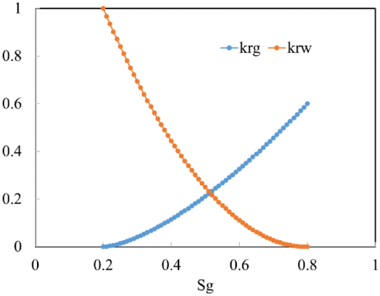
Figure 1: Relative permeability curve
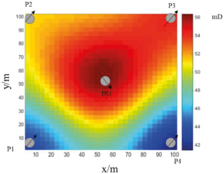
Figure 2: Reservoir example
The physical properties of the material are listed in Table 1, and the relative permeability curve is shown in Fig. 2. The relative permeability curve is depicted in Fig. 2. The finite difference method can be used to validate the accuracy of the results produced by this method. As illustrated in Fig. 3, this method’s accuracy is comparable to that of the finite difference method, with an error of less than 1% for a daily oil production curve of four single wells. As can be seen, both this method and the finite difference method have a water breakthrough time of 170 days, which is comparable. Following the water breakthrough, daily oil production decreased significantly. The final result indicated that, while daily oil production from wells P1 and P4 remained constant, daily oil production from wells P2 and P3 decreased to almost zero, which was consistent with the law that wells P2 and P3 had a higher permeability than wells P1 and P4. This demonstrates that the SPH method is accurate, does not require meshing, and has a higher degree of convergence and stability than traditional numerical simulation.


Figure 3: Daily oil production comparison of a single well
4.1 Influence of Smooth Kernel Function
SPH method itself has high accuracy, but its results are affected by smooth kernel function, which directly determines the calculation efficiency and accuracy. Lucy [2] used the bell function as the support domain function. After that, Gaussian kernel function [21], cubic spline function, and quartic spline function [22] were proposed successively. Using the above example, the reservoir model and parameters are consistent with the above example, and only the smooth kernel function calculated by the SPH method is changed.
As illustrated in Figs. 4 and 5, various smooth kernel functions have a significant effect on well P1’s daily oil production and block water cut. The Gaussian function fits the finite difference method perfectly for this demonstration. The bell function has a 175-day water breakthrough time, while the cubic spline function has a 170-day water breakthrough time. For the cubic spline function, water breakthrough occurs after 175 days. After 200 days, the block water cut for the Gaussian function is 0.3, while the block water cut for the other three functions is 0.8, indicating a significant difference in the block water cut values. It demonstrates that, in this particular case, the Gaussian function is more appropriate for this simulation.
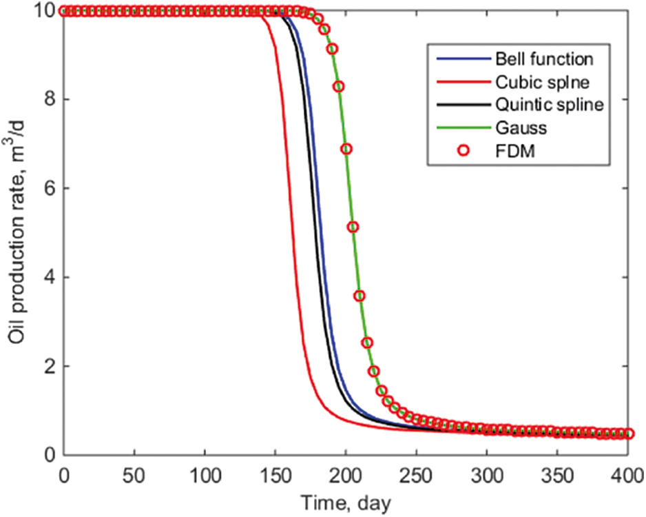
Figure 4: Comparison of oil production curve of P1
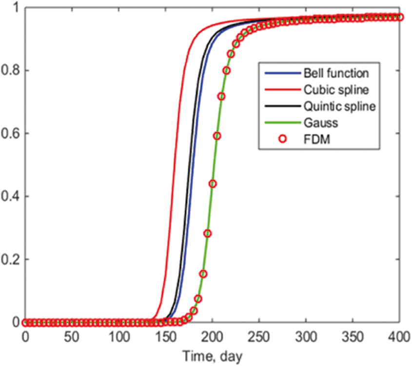
Figure 5: Water cut
4.2 Influence of Injection Production Ratio
The injection production ratio is crucial in calculating the actual production levels of a reservoir. The injection production ratio is critical for maximizing economic gain. To ensure that the simulation’s other physical parameters are consistent with the above calculation example, the injection volume is maintained at 40 m3/day, and the production volumes for each production well are set to 8 m3/day, 10 m3/day, 12 m3/day, and 14 m3/day, respectively, in this paper’s example of the above calculation.
As illustrated in Fig. 6 and 7, the water breakthrough time changes according to the amount of produced liquid under control. With a production rate of 14 m3/day, the block’s cumulative oil production can reach 9246 m3 in 400 days. If production is increased to 8 m3/day, however, the water breakthrough time is lowered to 170 days, and the block’s cumulative oil production can reach 6338 m3 in 400 days. As can be shown, the choice of an appropriate fixed liquid production method has a direct effect on the economic benefits of a piece of real estate within a given range. This is compatible with conventional wisdom and the method given in this paper, which illustrates its resilience.
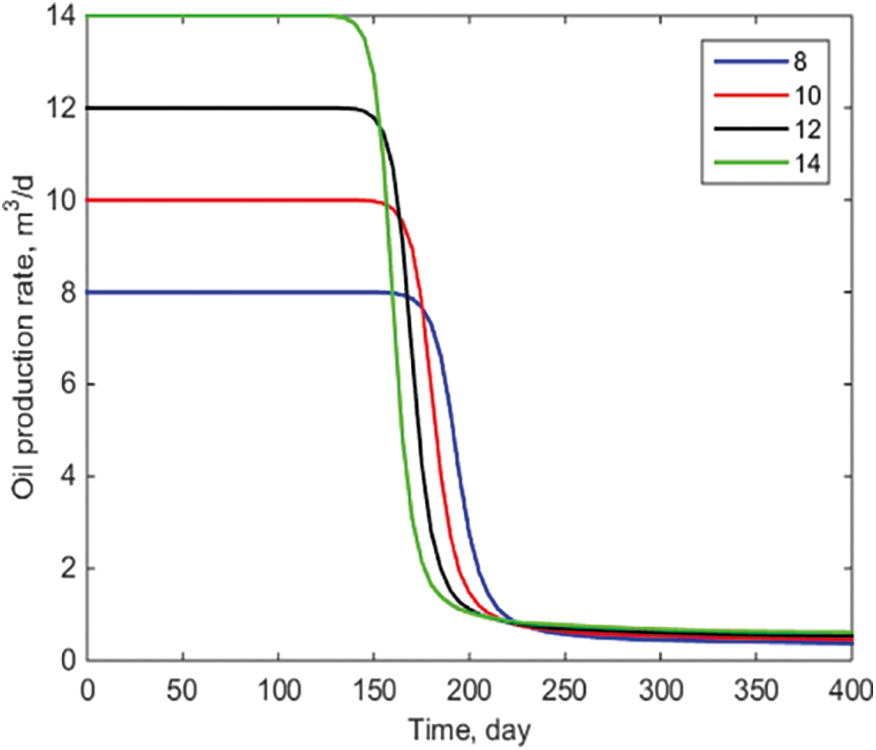
Figure 6: Comparison of oil production of P1
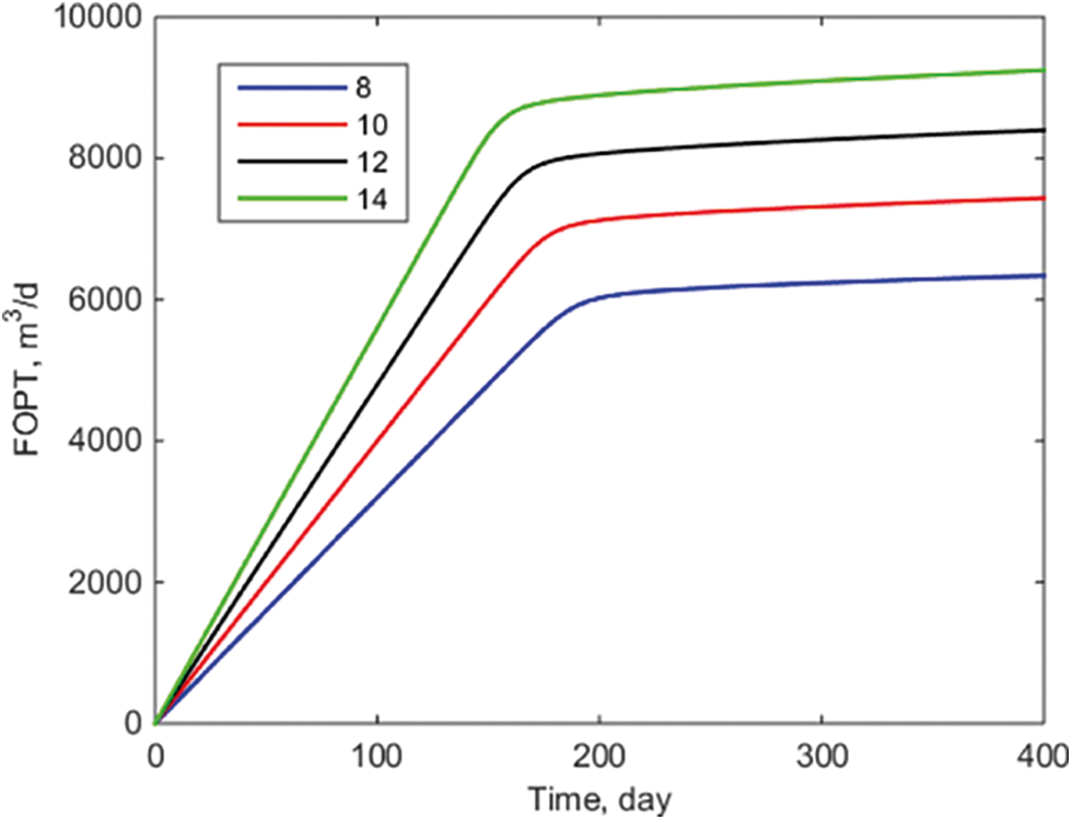
Figure 7: Cumulative oil production in block
4.3 Influence of Initial Formation Pressure
The initial pressure is a critical factor in determining daily oil production. The initial formation pressure can be used to evaluate the reservoir’s development potential and more intuitively reflect the reservoir’s oil phase conductivity. The initial formation pressures of 15 MPa, 20 MPa, 25 MPa, and 30 MPa are used in this paper for simulation, and the examples above are used to ensure that the other physical parameters match those in Table 1. The Gaussian function is used in the SPH method.
As illustrated in Fig. 8, when the initial formation pressure varies, the daily oil production of a single well remains consistent. This is primarily because, even with different initial pressures, oil production is determined by the pressure difference, as different initial formation pressures cannot affect daily oil production under conditions of constant liquid production. The water breakthrough time for well P1 has been maintained at approximately 150 days, and subsequent daily oil production has been maintained at 0.5 m3/day. This is consistent with conventional wisdom, demonstrating the validity of the SPH method in this paper.
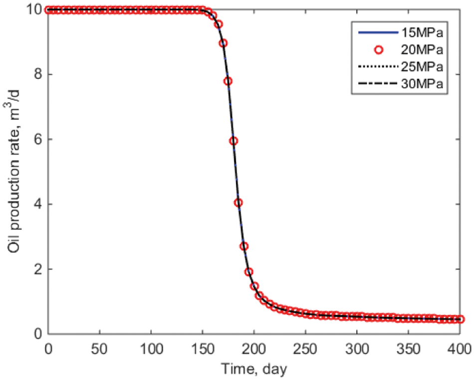
Figure 8: Daily oil production comparison curve of well P1
(1) This is the first time the SPH method has been applied to two-phase oil-water simulations. In comparison to the finite difference method, the example results show that this approach is correct, but it has a higher degree of stability because it does not require the development of a grid.
(2) This article analyzes the smooth kernel functions computed using various SPH algorithms. The Gaussian function has a block water cutoff of 0.3 at 200 days, while the other three functions have a block water cutoff of 0.8, with noticeable inaccuracy. It indicates that in this circumstance, the Gaussian function is more appropriate for the simulation.
(3) This article will evaluate the influence of various injection production ratios on real reservoir output. When 14 m3/day is established, the water breakthrough time is 130 days, and the cumulative oil production of the block can reach 9246 m3 in 400 days. When 8 m3/day is established, the period required for water breakthrough is decreased to 170 days, and the cumulative oil production of the block can reach 6338 m3 in 400 days. This is consistent with conventional wisdom, proving the method’s robustness in this research.
(4) This article examines the effect of initial formation pressure on daily oil production. A single well’s daily oil production is consistent regardless of initial pressure; well P1’s water breakthrough time is always around 150 days, and subsequent daily oil production is always 0.5 m3/day. This is consistent with the objective understanding that the major driver of oil-water two-phase flow is differential pressure in the reservoir.
Funding Statement: This work was supported by The China Postdoctoral Science Foundation (2021M702304) and Natural Science Foundation of Shandong Province (ZR2021QE260).
Conflicts of Interest: The authors declare that they have no conflicts of interest to report regarding the present study.
1. Du, M., Jing, J., Xiong, X., Lang, B., Wang, X. et al. (2022). Experimental study on heavy oil drag reduction in horizontal pipelines by water annular conveying. Fluid Dynamics & Materials Processing, 18(1), 81–91. DOI 10.32604/fdmp.2022.016640. [Google Scholar] [CrossRef]
2. Lucy, L. B. (1977). A numerical approach to the testing of the fission hypothesis. Astrophysical Journal, 8(12), 1013–1024. DOI 10.1086/112164. [Google Scholar] [CrossRef]
3. Li, M., Sun, J., Liu, D., Li, Y., Li, K. et al. (2020). A model for the optimization of the shale gas horizontal well section based on the combination of different weighting methods in the frame of the game theory. Fluid Dynamics & Materials Processing, 16(5), 993–1005. DOI 10.32604/fdmp.2020.010443. [Google Scholar] [CrossRef]
4. Verma,S., Aziz,K. (1996). Two-and three-dimensional flexible grids for reservoir simulation. ECMOR V-5th European Conference on the Mathematics of Oil Recovery, cp-101-00013. European Association of Geoscientists & Engineers. DOI 10.3997/2214-4609.201406874. [Google Scholar] [CrossRef]
5. Dicks, E. M. (1993). Higher order Godunov black-oil simulations for compressible flow in porous media. Citeseer. [Google Scholar]
6. Rao, X., Zhan, W., Zhao, H., Xu, Y., Liu, D. et al. (2021). Application of the least-square meshless method to gas-water flow simulation of complex-shape shale gas reservoirs. Engineering Analysis with Boundary Elements, 129(1), 39–54. DOI 10.1016/j.enganabound.2021.04.018. [Google Scholar] [CrossRef]
7. Xu, Y., Sheng, G., Zhao, H., Hui, Y., Zhou, Y. et al. (2021). A new approach for gas-water flow simulation in multi-fractured horizontal wells of shale gas reservoirs. Journal of Petroleum Science Engineering, 199(1), 108292. DOI 10.1016/j.petrol.2020.108292. [Google Scholar] [CrossRef]
8. Rao, X., Cheng, L., Cao, R., Jiang, J., Fang, S. et al. (2018). A novel green element method based on two sets of nodes. Engineering Analysis with Boundary Elements, 91, 124–131. DOI 10.1016/j.enganabound.2018.03.017. [Google Scholar] [CrossRef]
9. Zhao, H., Sheng, G. L., Huang, L. Y., Zhong, X., Fu, J. G. et al. (2021). Application of Lightning Breakdown Simulation in Inversion of Induced Fracture Network Morphology in Stimulated Reservoirs. International Petroleum Technology Conference, Virtual. DOI 10.2523/IPTC-21157-MS. [Google Scholar] [CrossRef]
10. Ginting, V. E. (2004). Computational upscaled modeling of heterogeneous porous media flow utilizing finite volume method (Doctor of Philosophy). College Station, TX: Texas A&M University. [Google Scholar]
11. Feng, Y., Liu, Y., Chen, J., Mao, X. (2022). Simulation of the pressure-sensitive seepage fracture network in oil reservoirs with multi-group fractures. Fluid Dynamics & Materials Processing, 18(2), 395–415. DOI 10.32604/fdmp.2022.018141. [Google Scholar] [CrossRef]
12. Malaspinas, O., Courbebaisse, G., Deville, M. (2007). Simulation of generalized Newtonian fluids with the lattice Boltzmann method. International Journal of Modern Physics C, 18(12), 1939–1949. DOI 10.1142/S0129183107011832. [Google Scholar] [CrossRef]
13. Tartakovsky, A. M., Meakin, P. (2005). Simulation of unsaturated flow in complex fractures using smoothed particle hydrodynamics. Vadose Zone Journal, 4(3), 848–855. DOI 10.2136/vzj2004.0178. [Google Scholar] [CrossRef]
14. Zhu, Y., Fox, P. J., Morris, J. P. (1999). A pore-scale numerical model for flow through porous media. International Journal for Numerical Analytical Methods in Geomechanics, 23(9), 881–904. DOI 10.1002/(ISSN)1096-9853. [Google Scholar] [CrossRef]
15. Simeunović, M., Steeb, H. (2019). Simulation of generalized Newtonian fluids with the smoothed particle hydrodynamics method. PAMM, 19(1), e201900494. DOI 10.1002/pamm.201900494. [Google Scholar] [CrossRef]
16. Ren, M., Shu, X. (2020). A novel approach for the numerical simulation of fluid-structure interaction problems in the presence of debris. Fluid Dynamics & Materials Processing, 16(5), 979–991. DOI 10.32604/fdmp.2020.09563. [Google Scholar] [CrossRef]
17. Liu, M., Liu, G. (2010). Smoothed particle hydrodynamics (SPHAn overview and recent developments. Archives of Computational Methods in Engineering, 17(1), 25–76. DOI 10.1007/s11831-010-9040-7. [Google Scholar] [CrossRef]
18. Randles, P., Libersky, L. D. (1996). Smoothed particle hydrodynamics: Some recent improvements and applications. Computer Methods in Applied Mechanics Engineering, 139(1–4), 375–408. DOI 10.1016/S0045-7825(96)01090-0. [Google Scholar] [CrossRef]
19. Libersky, L. D., Petschek, A. G., Carney, T. C., Hipp, J. R., Allahdadi, F. A. (1993). High strain Lagrangian hydrodynamics: A three-dimensional SPH code for dynamic material response. Journal of Computational Physics, 109(1), 67–75. DOI 10.1006/jcph.1993.1199. [Google Scholar] [CrossRef]
20. Shao, J. R., Li, H. Q., Liu, G. R., Liu, M. B. (2012). An improved SPH method for modeling liquid sloshing dynamics. Computers & Structures, 100–101, 18–26. DOI 10.1016/j.compstruc.2012.02.005. [Google Scholar] [CrossRef]
21. Monaghan, J. J., Lattanzio, J. C. (1985). A refined particle method for astrophysical problems. Astronomy Astrophysics, 149(1), 135–143. [Google Scholar]
22. Morris, J. P. (1996). A study of the stability properties of smooth particle hydrodynamics. Publications of the Astronomical Society of Australia, 13(1), 97–102. DOI 10.1017/S1323358000020610. [Google Scholar] [CrossRef]
 | This work is licensed under a Creative Commons Attribution 4.0 International License, which permits unrestricted use, distribution, and reproduction in any medium, provided the original work is properly cited. |