| Fluid Dynamics & Materials Processing |
DOI: 10.32604/fdmp.2022.020649
ARTICLE
Machine Learning-Based Prediction of Oil-Water Flow Dynamics in Carbonate Reservoirs
School of Geosciences, Yangtze University, Wuhan, 430100, China
*Corresponding Author: Xianhe Yue. Email: changjiangun@163.com
Received: 05 December 2021; Accepted: 01 March 2022
Abstract: Because carbonate rocks have a wide range of reservoir forms, a low matrix permeability, and a complicated seam hole formation, using traditional capacity prediction methods to estimate carbonate reservoirs can lead to significant errors. We propose a machine learning-based capacity prediction method for carbonate rocks by analyzing the degree of correlation between various factors and three machine learning models: support vector machine, BP neural network, and elastic network. The error rate for these three models are 10%, 16%, and 33%, respectively (according to the analysis of 40 training wells and 10 test wells).
Keywords: Carbonate rock; machine learning; support vector machine; fluid dynamics; neural network
At the moment, carbonate reserves are found around the planet. Around 40% of the world’s 236 big oil and gas fields are carbonate reservoirs, with 96 being carbonate reservoirs dominated by chert and dolomite reservoirs. Until present, carbonate oil and gas fields have been located and developed in almost 40 countries and over 60 sedimentary basins worldwide, and the reserves of these exploited carbonate fields have accounted for up to 65 percent of the world’s total original reserves.
Despite the fact that numerous scholars have investigated the oil and water dynamics of this sort of reservoir [1]. Some scholars proposed two models of fractured carbonate reservoirs with triple media. Li et al. examined the declining production characteristics of naturally fractured reservoirs, demonstrating a single pore media with a fractured fractal grid and a double pore media with a fractured fractal grid [2–4]. Wang [5] investigated the production variation of multi-media reservoirs and multi-media composite reservoirs in carbonate rocks under constant pressure production settings, employing transient decreasing production analysis as the theoretical foundation for the production variation law. Wang [5] examined the formation’s stress-sensitive characteristics and amended the usual stress-sensitive characterization equation by incorporating reservoir characteristics. A binomial capacity equation for anomalous high-pressure gas reservoirs was constructed using a modification of the stress-sensitive characterisation equation. The equation was used to calculate and anticipate the capacity of anomalous high-pressure gas reservoirs in the Yinggehai Basin, and the calculation findings indicated that stress sensitivity could not be ignored during gas field exploitation, as it would lower gas well capacity. Huang et al. [6] used a combination of experimental and theoretical methodologies to compare five commonly used stress-sensitive formulas. The finding was that a power-law formulation of the stress sensitivity characterisation equation for fractured reservoirs is possible. The results indicate that the stress sensitivity characterization equation is different for fractured reservoirs with varying degrees of fracture surface roughness and tortuosity, as well as varying degrees of formation stress sensitivity. And for dense reservoirs, the fracture permeability features are stronger, necessitating the employment of the power-law formula for characterization. Huang et al. [6] researched the fluid flow laws in low-permeability gas reservoirs and developed capacity calculation formulas for fractured horizontal wells, inclined fractures, and fractured horizontal wells with gas-water two-phase flow. The model was then evaluated using dynamic data from actual production wells, and the validation results indicated that the model had a high degree of applicability. Baghban et al. [7] and colleagues derived the pressure calculation equation and production prediction equation for gas wells in the presence of gas-water two-phase flow, providing theoretical evidence for dynamic production forecast of gas wells when the gas phase and water phase are identical. Although numerous research on the flow law and capacity evaluation of carbonate reservoirs have been done, the majority of them have focused on a single contributing factor.
We investigated the variation in output from production wells in multi-media reservoirs and multi-media composite reservoirs. However, due to the difficulties associated with poor matrix permeability and complex seam development in carbonate reservoirs, the application of these conventional production forecast methodologies frequently results in significant mistakes when estimating carbonate reservoirs. As a result, oilfield workers employ a variety of machine learning techniques in the fracturing process. For example, some scholars used a support vector machine algorithm to develop a quantitative prediction model of daily fluid production following fracturing, which serves as an effective reference for field fracturing work [8–12]. Li developed a mathematical model for predicting the output pattern of fracturing fluid in gas wells by ranking 26 variables affecting shale gas well production hierarchically using big data screening and analysis. Nejad et al. [13] evaluated all completion and fracture-related characteristics using a neural network model trained on multiple datasets and produced a model with oil and gas production as the output. Additionally, eight field wells were used to evaluate the model’s reliability. Tahmasebi developed data mining and machine learning algorithms to assist in identifying the optimal reservoirs for shale reservoirs, that is, locations with a high total organic carbon (TOC) content and fracturable brittle rocks [14]. Mohaghegh [15,16] used cutting-edge machine learning to analyze the McVey et al. [17] constructed, trained, and implemented an artificial neural network to evaluate and discuss the application of this new technology to hydraulic fracture design and evaluation. design and evaluation of fracturing. Zhu introduced an adaptive threshold denoising neural network model (ATD-BP) in 2017 for predicting production from high-dimensional small-scale shale gas reservoir alteration. The model initially removes noise using the adaptive threshold de-noising (ATD) algorithm, and then This model first removes noise using the adaptive threshold denoising (ATD) algorithm and then fits the reservoir modification data nonlinearly using a BP neural network to obtain a shale gas well production prediction model, which significantly improves the prediction’s accuracy and stability when compared to the traditional BP neural network model [18].
Beginning with the current state of carbonate reservoirs, the paper integrates and compares three machine learning methods, namely evaluation of support vector regression, BP neural network, and elastic network, in order to propose a carbonate production capacity prediction method based on support vector regression. This method can be used to forecast the future production capacity of carbonate development wells using geological and engineering data from existing carbonate wells.
2 Kinetic Influence Parameter Analysis
The gray correlation method is based on gray system theory and can be used to determine the degree of connection between numerous variables. The degree of correlation between several variables is determined by the correlation coefficients of the reference and comparison series. If the change trends of the reference and comparison series are inconsistent, the correlation degree is low; conversely, if the change trends of the reference and comparison series are consistent, the correlation degree is strong.
Gray correlation analysis is used to examine the gray correlation of each influencing parameter in order to determine the numerical link between the system’s parameters using a specific method. It is based on each factor’s sample data and uses gray correlation to quantify the strength, magnitude, and order of the link between components. The advantage of this strategy is that the concepts are straightforward, the loss caused by knowledge asymmetry may be significantly reduced, and the data requirements and workload are little. The following are the specific steps in the analysis.
Let
(1) Data causelessness
(2) Difference sequence notation
(3) Calculate the maximum difference k and the minimum difference k between the two levels
(4) Calculate the number of correlation coefficients
where
(5) Calculate the gray correlation
The Fig. 1 illustrates the relationships between discharge volume, horizontal section length, number of fracture sections, cumulative production months, fracture section spacing, average pumping stoppage pressure, design hydraulic half-seam length, cluster spacing, and production volume. The following connections exist between discharge volume, horizontal section length, number of fracturing sections, cumulative production months, spacing between fracturing sections, average stopping pressure, design hydraulic half-slit length, and cluster spacing: Correlation coefficients for four factors, including discharge volume, horizontal section length, number of fracturing sections, and cumulative production months, are greater than 0.6.
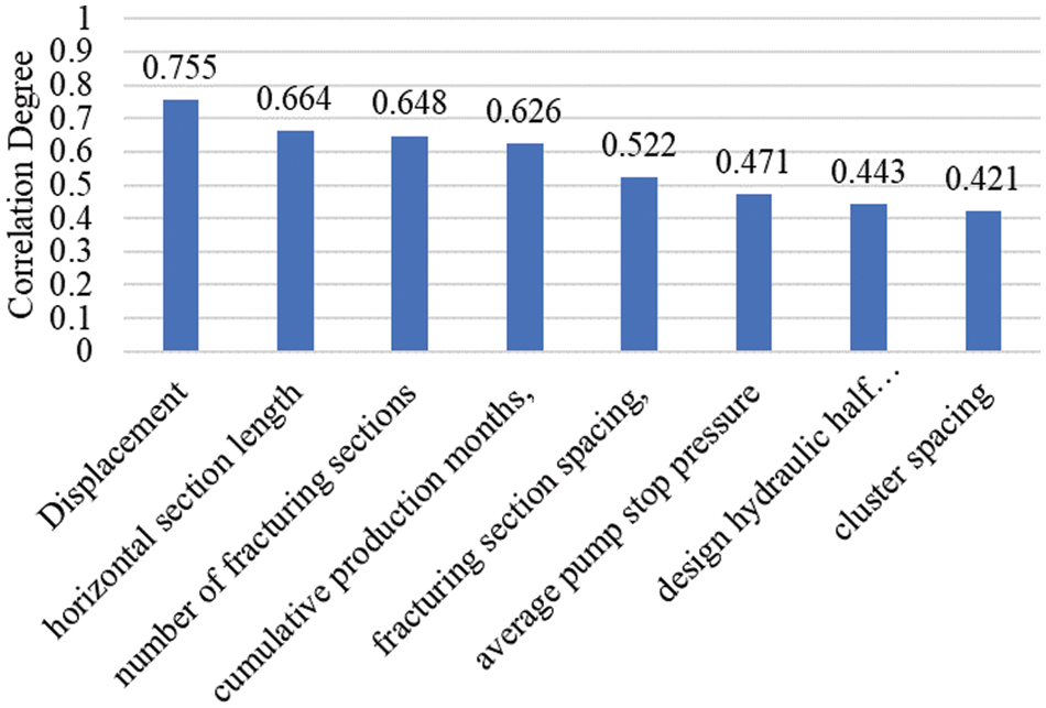
Figure 1: Relevance analysis
3 Machine Learning Model Preference
Since the actual fracturing sample data set is small and not suitable for machine learning methods based on large data samples, the three algorithms used are support vector machine regression, elastic network regression, and BP neural network for preferences, and the three models and parameter settings are briefly described below.
Elastic network regression (EN) is a fusion of Lasso regression and ridge regression, which is a standard linear regression with a canonical term, the squared deviation factor, added to make the optimization function into
An artificial neural network is a novel type of information processing network system developed on the basis of biological research that is capable of acquiring knowledge and solving problems through learning. It is an effective method for solving complex nonlinear problems via self-learning methods. The BP neural network (abbreviated BP) is a self-learning nonlinear fitting modeling technique that adapts and determines the connection weights of each neuron based on the input training samples. Between the input and output layers, further layers (one or more layers) of neurons are added. These neurons are referred to as hidden units since they have no direct link to the outside world. However, their state changes can impact the relationship between input and output, and each layer can contain multiple nodes. After numerous training sessions with the neural network system, the fitting information extracted from the sample data set is stored in the weights of each layer of the neural network. Finally, by combining the input data and weights, the required prediction value is obtained. We focus on the classical three-layer BP neural network model in this paper, which has the following structure diagram (Fig. 2).
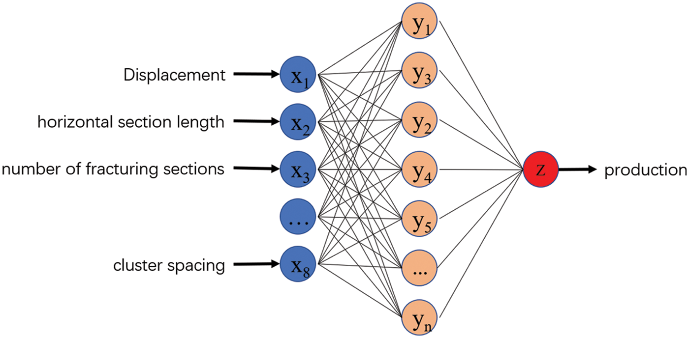
Figure 2: BP neural network structure
3.3 Support Vector Machine Regression
The core of support vector regression (SVR for short) is to discover the intrinsic connection between different data, and by fitting the data at high latitudes, the algorithm can obtain a formula that yields a new output value when the input value is changed. the major difference between SVR regression and traditional regression methods is that traditional regression methods require that the prediction is considered correct when and only when the f(x) of the regression is exactly equal to y, while support vector regression is considered correct as long as f(x) deviates from y within a certain range. Specifically, a threshold α is set and the loss of data points with
For SVR, the most important parameter is the kernel type, which generally includes linear kernel, polynomial kernel, hyperbolic tangent kernel, and Gaussian Radial Basis Function. Because of the nonlinearity problem of reservoir data, RBF is chosen as the kernel function, and the parameters that mainly affect RBF are penalty factor C and kernel parameter γ.
As shown in the figure, the method in Grid Search is used to determine the optimal penalty factor C and the kernel parameter γ of the support vector machine algorithm, that is, to experiment the effect of each pair of parameters in turn in a two-dimensional parameter matrix composed of C and γ. Firstly, the optimal penalty factor C and the kernel parameter γ are given in the range of (
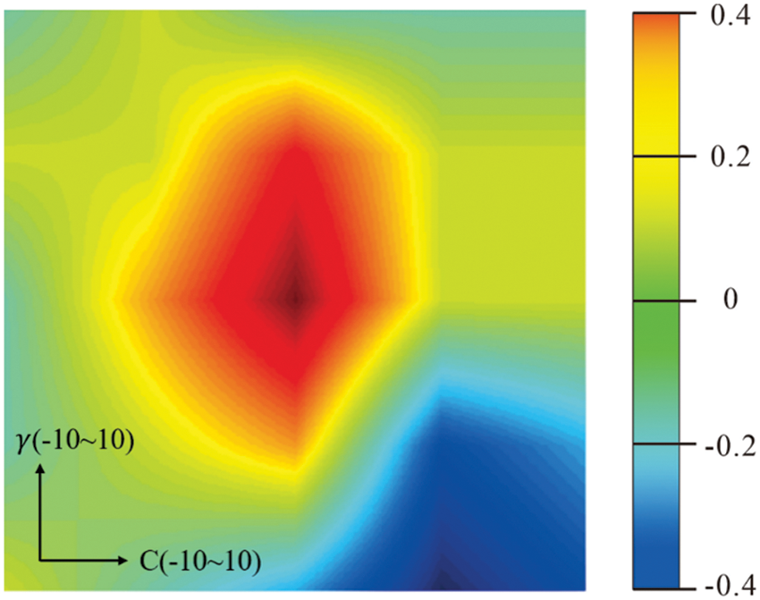
Figure 3: Parameter optimization results
To evaluate the strengths and weaknesses of the regression effects of the three models for the fracturing optimization problem, a cross-validation approach was utilized. Fifty wells were selected, 40 of which were used as training set data, and the remaining 10 wells were used as test set data. The support vector machine model, BP neural network model, and elastic network model were trained respectively, and the 10 wells data were used as input to predict their post-frac production, and the model regression prediction results are shown in Fig. 4 below, with the errors shown in Table 1 below (Fig. 5).
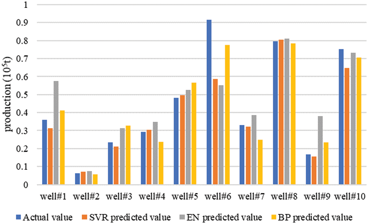
Figure 4: The prediction effect of the three models
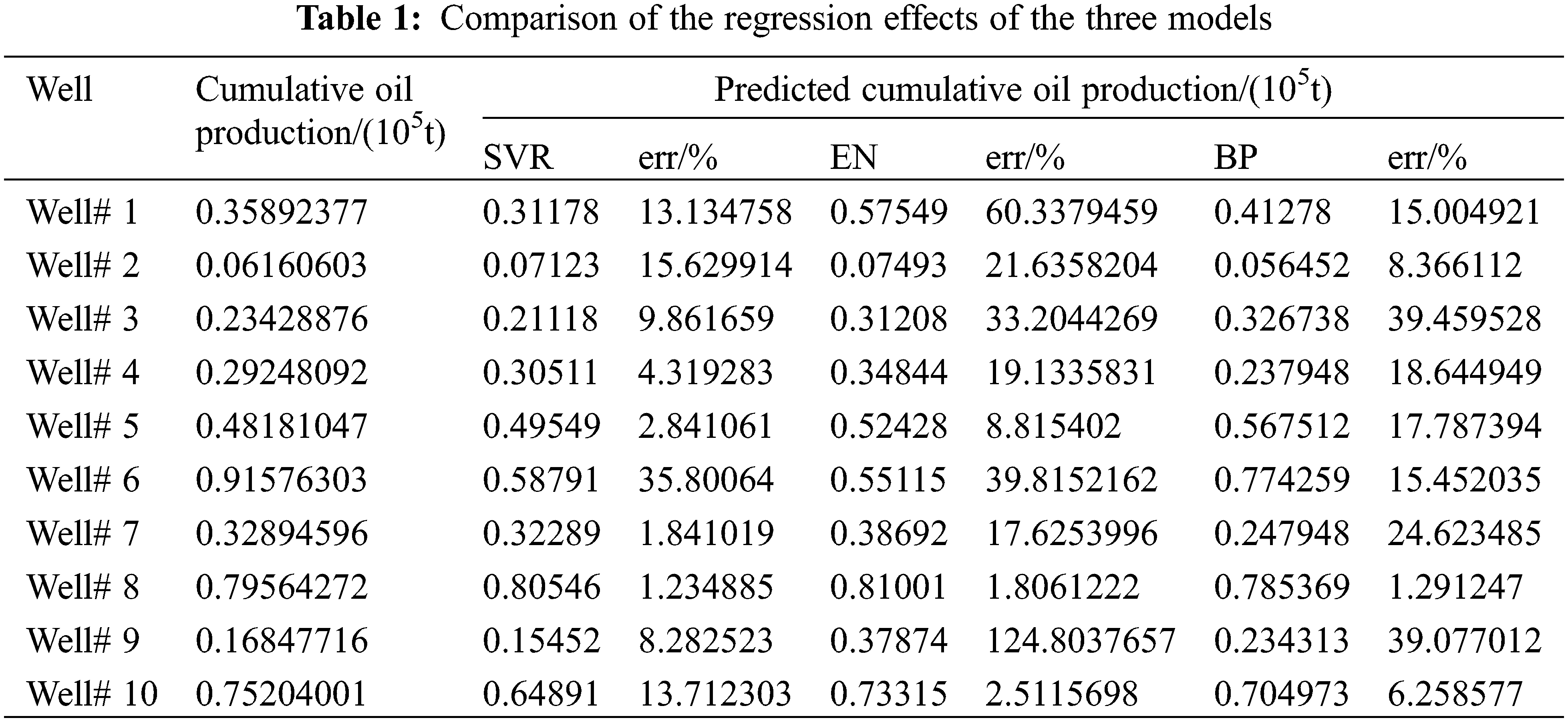
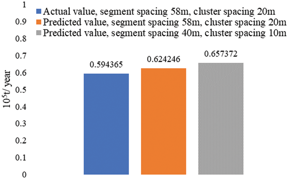
Figure 5: Production comparison
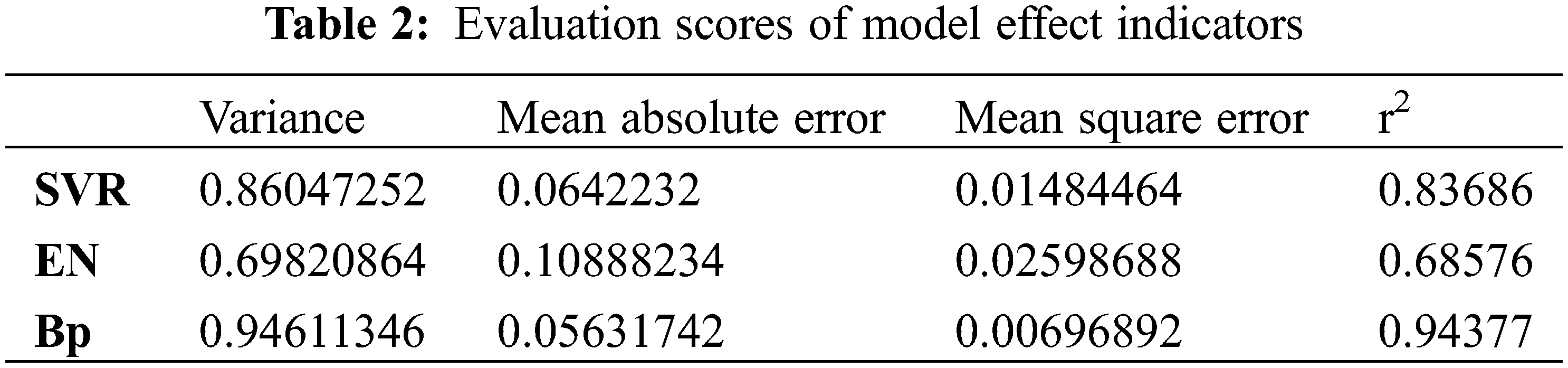
Table 1 shows the average error of the three models of support vector machine model, BP neural network model, and elastic network model are, 0.10665805, 0.185965266, and 0.329689252, respectively, where the average error of SVR is the smallest. Then the four evaluation indexes of variance, mean absolute error, mean squared error, and coefficient of determination of the regression model were examined to check the effectiveness of the machine learning model. The results are shown in Table 2 below, and the comparison can be found that support vector regression and BP neural network are more effective than elastic network regression.
Based on the above-evaluated results, the support vector machine algorithm has the best overall performance, so the support vector machine algorithm was selected for exploratory analysis of fracturing effects in carbonate reservoirs.
One well data was selected and the existing formation and construction parameters of the well were input into the completed production prediction model trained using the SVR algorithm. It is known that the actual production capacity of the well is about 0.594365 (105 tons/year), while the model predicts the production value of 0.624246 (105 tons/year), and the comparison shows that the actual value is close to the model prediction, and the prediction error is about 5%. According to the above analysis of model input parameters and yield, we choose to adjust the model input parameters, including adjusting the segment spacing from 58 m to the optimal segment spacing of 40 m and adjusting the cluster spacing from 20 m to the optimal cluster spacing of 10 m, then the prediction result is 0.657372 (million tons/year) when the input parameters are brought into the model at this time, which can improve the cumulative oil production by about 10.6% after optimization.
(1) The magnitude of the factors impacting the capacity of carbonate wells was calculated using the gray correlation approach. Correlation coefficients for four criteria, including discharge volume, horizontal section length, number of broken sections, and total production months, were larger than 0.6, indicating the largest effect.
(2) The three machine learning methods of support vector regression, BP neural network, and elastic network were compared and evaluated, and the results indicated that the support vector machine algorithm performs the best overall and offers the most unique advantages for small samples and non-linear complex data.
(3) Using an actual oil well as input to a support vector regression-trained production prediction model, it was determined that the error between predicted and actual production was approximately 5%, while cumulative oil production could be increased by approximately 10% after optimization by modifying the construction parameters.
Funding Statement: The authors received no specific funding for this study.
Conflicts of Interest: The authors declare that they have no conflicts of interest to report regarding the present study.
1. Li, Y., Wu, F., Li, X., Tan, X., Hu, X. et al. (2017). Displacement efficiency in the water flooding process in fracture-vuggy reservoirs. Journal of Petroleum Exploration Production Technology, 7(4), 1165–1172. DOI 10.1007/s13202-017-0321-7. [Google Scholar] [CrossRef]
2. Gao, S., Liu, H., Ren, D. (2015). Deliverability equation of fracture-cave carbonate reservoirs and its influential factors. Natural Gas Industry, 35(9), 48–54. DOI 10.3787/j.issn.1000-0976.2015.09.07. [Google Scholar] [CrossRef]
3. Li, L., Yao, J., Li, Y., Wu, M., Zeng, Q. (2014). Productivity calculation and distribution of staged multi-cluster fractured horizontal wells. Petroleum Exploration and Development, 41(4), 504–508. DOI 10.1016/S1876-3804(14)60058-6. [Google Scholar] [CrossRef]
4. Liu, C. (2017). Dynamic evaluation and characteristic analysis of the capacity of single wells in landphase dense reservoirs (Master Thesis). China University Of Petroleum (Beijing). https://kns.cnki.net/kcms/detail/detail.aspx?dbcode=CMFD&dbname=CMFD201901&filename=1019808077.nh&uniplatform=NZKPT&v=vpkeV85nqvFMVzldt5tbdWW2uyx1-tas4aN37cG-HX7G4ci3U-iv471kjecezeF1. [Google Scholar]
5. Wang, S. (2016). Study on the method of analysis of the decreasing yield of transient in carbonate rock multi-media reservoir single well (Master Thesis). Southwest Petroleum University. https://kns.cnki.net/kcms/detail/detail.aspx?dbcode=CMFD&dbname=CMFD201702&filename=1017108172.nh&uniplatform=NZKPT&v=iOLn9MfJi3J-3MIZ0zXglI349zJuYruUQNEkxdgN92sIkVmJOkZQGrJ9maNlCbv-. [Google Scholar]
6. Huang, S., Ding, G., Wu, Y., Huang, H., Lan, X. et al. (2018). A semi-analytical model to evaluate productivity of shale gas wells with complex fracture networks. Journal of Natural Gas Science and Engineering, 50(12), 374–383. DOI 10.1016/j.jngse.2017.09.010. [Google Scholar] [CrossRef]
7. Baghban, A., Abbasi, P., Rostami, P. (2016). Modeling of viscosity for mixtures of Athabasca bitumen and heavy n-alkane with LSSVM algorithm. Petroleum Science Technology, 34(20), 1698–1704. DOI 10.1080/10916466.2016.1219748. [Google Scholar] [CrossRef]
8. Zhao, X. (2016). SVM deep geo-stress prediction model. Special Oil and Gas Reservoirs, 23(1), 139–141. DOI 10.3969/j.issn.1006-6535.2016.01.032. [Google Scholar] [CrossRef]
9. Zhang, P., Wu, T., Li, Z., Li, Z., Wang, J. et al. (2020). Application of BP neural network method to predict the stress sensitivity of ultra deep carbonate reservoir in Shunbei Oilfield. Oil Drilling & Production Technology, 42(5), 622–626. DOI 10.13639/j.odpt.2020.05.016. [Google Scholar] [CrossRef]
10. Tian, L., He, S. L., Gu, D. H., Zhang, H. L. (2008). Application of neural network technique for productivity evaluation in changqing gasfield. Journal of Oil and Gas Technology, 30(5), 106–109. [Google Scholar]
11. Zhang, Y., Gong, W., Yu, Y. (2019). Predicting snow depth during strong rain and snowfall processes using machine learning techniques. Science Technology and Engineering, 19(15), 57–69. [Google Scholar]
12. Zhao, R., Shi, J., Zhang, X., Li, J., Miao, G. (2019). Research and application of the big data analysis platform of oil and gas production. International Petroleum Technology Conference, Beijing, China. DOI 10.2523/IPTC-19458-MS. [Google Scholar] [CrossRef]
13. Nejad, A. M., Sheludko, S., Shelley, R. F., Hodgson, T., McFall, R. et al. (2015). A case history: Evaluating well completions in the Eagle Ford Shale using a data-driven approach. SPE Hydraulic Fracturing Technology Conference, The Woodlands, Texas, USA. DOI 10.2118/173336-MS. [Google Scholar] [CrossRef]
14. Tahmasebi, P., Javadpour, F., Sahimi, M. (2017). Data mining and machine learning for identifying sweet spots in shale reservoirs. Expert Systems with Applications, 88(1), 435–447. DOI 10.1016/j.eswa.2017.07.015. [Google Scholar] [CrossRef]
15. Mohaghegh, S. D. (2016). Fact-based re-frac candidate selection and design in shale-a case study in application of data analytics. SPE/AAPG/SEG Unconventional Resources Technology Conference, San Antonio, Texas, USA. DOI 10.15530/URTEC-2016-2433427. [Google Scholar] [CrossRef]
16. Mohaghegh, S. D., Gaskari, R., Maysami, M. (2017). Shale analytics: Making production and operational decisions based on facts: A case study in marcellus shale. SPE Hydraulic Fracturing Technology Conference and Exhibition, Woodlands, Texas, USA, OnePetro. DOI10.2118/184822-MS. [Google Scholar] [CrossRef]
17. McVey, D. S., Mohaghegh, S., Aminian, K., Ameri, S. (1996). Identification of parameters influencing the response of gas storage wells to hydraulic fracturing with the aid of a neural network. SPE Computer Applications, 8(2), 54–57. DOI 10.2118/29159-PA. [Google Scholar] [CrossRef]
18. Zhu, H., Kong, D. Q., Xu, Q. (2017). Shale gas production prediction method based on adaptive threshold denoising BP neural network. Science Technology and Engineering, 17(31), 128–132. [Google Scholar]
 | This work is licensed under a Creative Commons Attribution 4.0 International License, which permits unrestricted use, distribution, and reproduction in any medium, provided the original work is properly cited. |