| Fluid Dynamics & Materials Processing |
DOI: 10.32604/fdmp.2022.019788
ARTICLE
A Model for the Connectivity of Horizontal Wells in Water-Flooding Oil Reservoirs
1Cooperative Innovation Center of Unconventional Oil and Gas (Ministry of Education & Hubei Province), Yangtze University, Wuhan, 430100, China
2School of Petroleum Engineering, Yangtze University, Wuhan, 430100, China
3Key Laboratory of Drilling and Production Engineering for Oil and Gas, Wuhan, 430100, China
4Tianjin Branch of CNOOC, Ltd., Tianjin, 300459, China
5Oilfield Technology Service Company, Xinjiang Oilfield Company, PetroChina, Karamay, 834000, China
*Corresponding Author: Fankun Meng. Email: mengfk09021021@163.com
Received: 15 October 2021; Accepted: 02 December 2021
Abstract: As current calculation models for inter-well connectivity in oilfields can only account for vertical wells, an updated model is elaborated here that can predict the future production performance and evaluate the connectivity of horizontal wells (or horizontal and vertical wells). In this model, the injection-production system of the considered reservoir is simplified and represented with many connected units. Moreover, the horizontal well is modeled with multiple connected wells without considering the pressure loss in the horizontal direction. With this approach, the production performance for both injection and production wells can be obtained by calculating the bottom-hole flowing pressure and oil/water saturation according to the material balance equation and a saturation front-tracking equation. Some effort is also provided to optimize (to fit known historical production performances) the two characteristic problem parameters, namely, the interwell conductivity and connected volume by means of a SPSA gradient-free algorithm. In order to verify the validity of the model, considering a heterogenous reservoir, three conceptual examples are constructed, where the number ratio between injection and production wells are 1/4, 4/1 and 4/5, respectively. It is shown that there is a high consistency between simulation results and field data.
Keywords: Connectivity model; horizontal well; production performance; interwell connectivity; connected volume
Currently, most mature oilfields have entered into the middle or late stages of water-flooding development with high water cut, and some of them are developed by horizontal wells. However, many of those horizontal wells are now facing the problems of high water cut, low oil recovery, serious water channeling, and prominent injection-production contradiction. Therefore, it is urgent to establish an efficient connectivity analysis method to clarify the connectivity between horizontal injection and production wells, and to guide the subsequent injection and production system adjustment, profile control and water shut off operations [1–4].
The traditional methods to study interwell connectivity mainly include well test, tracer test, numerical simulation, interwell microseismic method and mathematical methods. In 1966, Blasingame et al. [5] put forward the pulse well test analysis theory to study reservoir connectivity and gave the interpretation method of tangent method, but only solved the interpretation problem under isochronous conditions. Therefore, Blasingame et al. [6] improved the theory in 1975. In 2006, Zhang et al. [7] tried to combine the tracer detection technology with the reservoir numerical simulation technology to evaluate the connectivity between oil and water wells in fractured low permeability reservoir. However, the accuracy and reliability of the tracer detection method are greatly affected by the mutual interference between tracers, the compatibility between tracers and reservoir conditions, the detection sensitivity, etc. Moreover, the cost is usually very high. In 2013, according to the derived connectivity through the systematic analysis on the production data, Xu et al. [8] established a fine geological model to determine the type of flow unit in a single channel sand body. However, the numerical simulation method generally requires very accurate dynamic and static data, so the amount of work is large. In 2007, Du et al. [9] applied the microseismic monitoring technology to analyze the production dynamics and to evaluate the fracturing operation. However, interwell microseismic is generally used in the early stage of development, and the procedure is complex. In 2016, Xia et al. [10] used local empirical mode decomposition (LMD) to denoise the production data, and applied Gaussian estimation to solve the multiple linear regression model that considers the time lag. Nevertheless, the calculation is complicated and multiple cycles are required.
To resolve the shortcomings of the above-mentioned methods. New models such as correlation analysis model, multiple regression model, capacitance model and system analysis model are proposed based on field injection and production data to study the interwell connectivity. These simulation methods are easier to learn and less time-consuming, therefore, are widely used in the oilfield. For example, in 1996, Refunjol [11] proposed a technique to characterize reservoir connectivity by integrating reservoir geology, tracer data with Spearman rank correlation coefficient. In 1995, according to the interwell interaction characterized by the Spearman rank correlation coefficient of flux between paired well, Heffer et al. [12] put forward a new method to determine the flow directivity index. However, they overlooked the time lag-effect. In 1997, according to a specific characteristic property that is very similar to the injection-production interwell connectivity, Jansen et al. [13] also proposed an analysis method to deal with the reservoir properties with the interpolation method. In 1998, Panda et al. [14] also applied the artificial neural network model to study the connectivity between injection and production wells, and the obtained interwell relationships can be used to verify geological features, such as sealing faults and pinch-out points. In 1999, Soeriawinata et al. [15] established a correlation analysis model that considers the superposition principle of multiple injection wells, and the effects of superposition and destructive interferences are also considered in this model. In 2003, Albertoni et al. [16] established a multiple linear regression model (MLR) based on dynamic data and multiple linear regression method. In 2008, Dinh et al. [17] proposed a new model that uses well bottom-hole flowing pressure as input and output variables based on the MLR model. Subsequently, Dinh et al. [18] proposed an improved model, which included the concept of more stable interwell permeability as a model inversion parameter. In 2006, Yousef et al. [19,20] proposed a quantity calculation method named as capacitance resistance model (CRM) for the vertical interwell connectivity based on the production and injection rates. The capacitance model is an improved model that considers the delay of injection velocity and can offer a better way to demonstrate interwell connectivity. In 2007, Lake et al. [21] used a power-law relationship model to predict the oil production rate and carried out production history fitting and production optimization research. In 2009, Sayarpour et al. [22] extended the studies for CRM models, and established three different improved forms, such as CRMT, CRMP, and CRMIP, which have been applied in diverse block examples. In 2018, Naudomsup et al. [23] applied the CRM model to simulate the movement of tracers. In 2011, by regressing the velocity, initial reservoir pressure and bottomhole pressure data with multiple linear regression method, Nguyen et al. [24] proposed a new method to obtain the unique estimates of interwell connectivity, pore volume and productivity indexes of primary and secondary oil production. The problem was solved by analyzing the simplified integral equation of continuous material balance. Their method successfully quantified the flow resistance between capacitance, productivity index (PI) and well pairs. In 2021, Yousefi et al. [25] modified capacitance-resistance model (or M-CRM as a physical approach) through the combination of least square support vector machine and multiple linear regression (as a statistical approach) which are utilized for two immiscible gas injection cases. In these cases, the interwell connectivity is predicted and producer total rate is estimate.
In order to better reflect the dynamic changes of flow field and characteristics of inter-well connectivity parameters for water flooding reservoirs, Zhao et al. [26,27] proposed a novel data-driven model named as INSIM. In their model, the injection-production system is discretized into several interwell connected units and each unit is characterized by two characteristic parameters, conductivity and control volume. Material balance equation and saturation front-tracking equation for single connected unit are applied to calculate the bottom-hole flowing pressure and oil/water saturation and thereafter to obtain the oil-water production dynamic at each well point. Moreover, automatic inversion of model parameters is realized by integrating projection gradient algorithm with dynamic fitting. INSIM is developed with traditional mathematical model, but the computational method has been changed hugely to increase the calculation on injection-production dynamics. In 2014, Zhao et al. [26] calculated the oil/water dynamics with this connectivity model and in 2016, Zhao et al. [27,28] proposed a semi-analytical method which is suitable to calculate water saturation on the condition of changing flowing direction. In 2017, Guo et al. [29] obtained more accurate water cut data by using front tracking method to better solve the front saturation distribution equation with Buckley-Leverett (B-L) theory.
The current INSIM model can quickly and effectively reflect the connectivity relationship between vertical wells according to the actual injection-production data. But its applications in horizontal wells have not been reported yet. In 2020, Yao et al. [30] developed a composite model to model the fluid flow in unconventional reservoirs with MFHWs under various heterogeneity conditions and utilized solutions. The presented model is employed to analyze two sets of production data from fractured horizontal wells in heterogeneous conditions. However, the connectivity between horizontal wells is not evaluated yet. Considering the fact that horizontal wells are used broadly in oilfields to boost the oil production, establishing a new interwell connectivity model to study the inter-well connectivity between horizontal wells or between horizontal wells and vertical wells is urgent and meaningful. In this paper, the horizontal well is equivalently substituted by multiple connected nodes without considering the pressure loss in the horizontal direction. After the bottom-hole pressure and water/oil saturation are calculated and the actual dynamics are fitted with optimization algorithm, the formation parameters can be inversely calculated, and the real time interwell connectivity and production dynamics are reflected. In addition, the reliability of this model is verified by comparing the resulted water allocator and future production dynamics with the Eclipse model and the practicability of the model is confirmed by a case study to guide the development and the adjustment of actual oilfield.
2 Interwell Connectivity Model
In order to reduce the complexity of the model, the reservoir with multiple injection and production wells is simplified into a series of interwell connected units (Fig. 1). Herein, the vertical well is equivalent to one node and the horizontal well is equivalent to three nodes (Fig. 2). In Fig. 2, the red and the blue circles represent the connected units between the two nodes. To distinguish the units for different well types, different colors are used. Each connected unit can be characterized by two characteristic parameters: interwell conductivity and connected volume. The interwell conductivity reflects the seepage capacity of fluid in the connected unit, while the connected volume represents the effective pore volume of the interwell connected unit. Firstly, the material balance equation for each separate connected unit is established. Then, the pressure is obtained and the interwell flow rate is calculated by assuming constant production rate or constant pressure. After that, oil-water front propulsion theory is combined with the saturation tracking method to obtain production performance index of each well point.

Figure 1: Interwell connected unit

Figure 2: Equivalent nodes of horizontal wells
2.1 Material Balance Equation and Pressure Calculation
The compressibility of fluid and rock is considered and while he capillary force is ignored, the material balance equation for horizontal well h is:
where h,i is the well serial number; m is the node serial number; N is the number of injection/production wells; Nh is the node number of well h; Th,i,m is the conductivity between node m of well h and well i, m3/(d⋅MPa); Ct,h,m is the comprehensive compressibility of well h, MPa−1; Vp,h,m is the connected volume between node m of well h and well i, m3; t is the production time, d; pi is the average pressure in the drainage area of well i, MPa−1; ph is the average pressure in the drainage area of well h, MPa−1; qh is flow velocity of well h, and the positive value means inflow while negative value is outflow, m3/d.
Namely:
After implicit difference:
The conductivity and connected volume can be estimated based on the pressure or saturation of the last time node according to percolation theory:
where hh,i,m is the average effective thickness of m node of h well and i well, m; λh,i,m is the fluidity between the mth node of well h and well i, 10−3μm2/(mPa⋅s).
where λh is the mobility of mth node of well h, 10−3 μm2/(mPa⋅s); Kh,i,m is the average permeability of node m of well h and well i, 10−3 μm2; Kro and Krw is the relative permeability of oil and water, respectively; μo and μw are the oil and water viscosity, respectively, mPa⋅s.
Since there are two internal boundary conditions, constant production rate and constant pressure, therefore, two cases may occur in the actual simulation.
2.1.1 Constant Production Rate Production
As for constant production rate production,
where
The pressures of time node n and time node n + 1 is expressed as following:
The pressure of each well point at time node n + 1 can be obtained from Eq. (5), so the flow distribution in each connected unit is obtained:
where Qh,i,m is the velocity between node m of well h and well i.
2.1.2 Constant Pressure Production
As for constant pressure production, the bottom-hole flowing pressure is constant, and the production indexes of each well can be obtained by superimposing the production indexes in different connected direction. The control boundary of well h and well i is shown in Fig. 3, so the production index in this direction obtained by percolation theory [31] is:
where Jh,i,m is the production index in the connection direction between the m node of the h well and the i well, m3/(d⋅MPa); θh,i,m is the sector radian of connected unit, rad; hh,i,m is the average effective thickness of node m of well h and well i, m; rh is the wellbore radius of well h, m; sh is skin factor of well h.

Figure 3: Single well control volume diagram
However, the production index obtained with percolation theory is only reliable for steady-state and quasi-steady-state seepage. A new production index for unsteady seepage is deduced by the analytical method. In this part, the pressure difference is regarded as the difference between the average pressure in the control area and the bottom hole pressure: The new production index is obtained with Laplace numerical inversion, which includes the time term in the formula. Therefore, this solution method is more accurate than the approach which assumes the production index has no relationship with time.
Assume that the pressure at the control boundary of well h is pe, then the seepage equation is expressed as:
where K is permeability, mD; p is pore pressure, MPa; x is a position variable, m; ϕ is porosity, dimensionless; Ct is the comprehensive compression coefficient, MPa−1; μ is fluid viscosity, mPa⋅s; t is the time, d; α is the unit conversion coefficient. The value 11.57 is used in this paper.
Constant pressure for outer boundary:
Constant production for internal boundary:
where qi is the oil production rate, m3/d; A is the flow cross-sectional area, m2, β is the unit conversion factor, 0.0864. Herein,
The pseudo pressure is defined as the difference between boundary pressure and pore pressure:
And the seepage equations are converted to:
Perform Laplace transform on t, then:
Thus:
Assume:
Then the general solution of the seepage equation is:
The derivative is:
Substitute Eqs. (19) and (20) into the boundary conditions in Eq. (17):
Then, A and B can be obtained:
The pseudo pressure at any point can be expressed as:
The pseudo pressure at the well point is:
The simplified form is:
Apply Stehfest numerical inversion, then:
where:
k = 1, 2, ……, N (N = 8).
Further simplify the equation:
The bottom hole pressure is:
According to Eq. (28), the average pressure in the control unit is:
Thus:
The Production index can be defined as:
Substitute Eq. (33) into Eq. (34):
According to the definitions, conductivity (interwell conductivity) and connected volume (single well control volume) are expressed as:
Hence:
The production index is:
Adjust well spacing and represent it with L1, the conductivity and connected volume are:
The coefficient ε is:
The production index can be expressed as:
Therefore:
where
The overall production index of Well h is:
Since
where pwf,h is the bottom hole flowing pressure of well i, MPa.
Therefore, the implicit difference form of the material balance equation is:
The simplified form is:
where
Then the pressures at time node n and time node n + 1 expressed in the matrix form are as following:
The flow rate distribution of each connected unit is obtained from Eq. (6), and the single well injection or production volume is calculated by Eq. (43).
The injection or production volume of each horizontal well node is:
where WLPRm is the injection or production volume of each horizontal well node.
Since negative flowing bottomhole pressure may be obtained under constant production rate mode, a lower limit of flowing bottomhole pressure should be set. When the flowing bottomhole pressure is smaller than the limit, the production mode should be changed to constant pressure production mode, and the lower limit is regarded as the actual flowing bottomhole pressure.
2.2 Water Saturation Front Tracking
The fractional flow of oil and water are obtained by saturation front tracking calculation. For one-dimensional water flooding case, the saturation front can be tracked by solving the B-L front saturation distribution equation.
The water saturation of the x point (the distance between the x point and the injection end is x) and the total flow rate demonstrate the following relationship:
where x0 is the location of the inflow point, m; Qin is the cumulative injection volume, m3; fw is the water cut; Sw is the water saturation at the x point.
Suppose that xs is the upstream node of x, then:
Subtract Eq. (51) from Eq. (52), we can get:
where
The field site, measures such as convert oil well to water injection well and well shut-in may be implemented, in which case the pressure distribution and flowing direction may change significantly. Hence, if the upstream node and the downstream node are switched, the value of Qin should be the dimensionless cumulative injection after pressure change.
In order to ensure the stability of calculation, both forward and reverse flow are considered, and the minimum saturation values of the current time node and the previous time node for the researched node are taken (assume that well i is the upstream node of well h).
Therefore, Eq. (50) is corrected as:
where
After
The above-mentioned water saturation tracking method is called upstream weight method, which is limited to the case when node water saturation is greater than the front water saturation. While when the node saturation is lower than the front water saturation, the Eq. (51) is no longer applicable. The time-lag effects of the water front breakthrough would be more obvious, and the increase in water cut after breakthrough will be faster than the real situation.
The movements of the iso-saturation plane in the connected unit are similar to the propagation law of the wave. Thus, the saturation distribution problem can be transformed to the Riemann problem and be solved with the shock-wave theory, as shown in Fig. 4.

Figure 4: Shock wave tracking of water saturation
According to the B-L theory, the moving speed of any iso-saturation surface is equal to the ratio between water cut and water saturation. For example, in a connected unit, the initial saturations for the upstream well point i and downstream well point m are greater than the front saturation, as shown in the blue line in Fig. 4. In the saturation distribution of the connected element, the velocity for any two saturation profiles is
When the saturation of the upstream node i locates between the front saturation and the irreducible water saturation while the saturation of the downstream node m equals to the irreducible water saturation, the advancing speed of the saturation surface in the connected element can be expressed as following according to the shock-wave theory:
Assume that the flow time required for the movement of saturation surface to upstream node i is ti, the water saturation of node m would be:
When tivh,i,m > Lh,i,m, the movement of saturation surface from the upstream node i to the downstream node m, and the water cut of node i can be calculated by the fractional flow equation. When tivh,i,m < Lh,i,m, the saturation surface will not move from the upstream node i to the downstream node m, and the downstream node m is still saturated with pure oil.
Thus, the improved node saturation calculation equation based on the shock-wave theory is:
After obtaining the water-cut of each node, the oil production, water production and water injection allocator can be further calculated. The proposed connectivity model has several advantages: ① Horizontal wells are equivalently substituted by several nodes. ② The new production index obtained by analytical method is more accurate than that obtained by seepage theory. ③ The saturation tracking equation solved by the shock wave theory can give consideration to saturation distribution both in the high water-cut period and low water-cut stage. ④ The solution of saturation tracking equation with semi-analytical method is faster than the traditional reservoir simulation.
2.3 Inversion of Characteristic Simulation Parameters
The dynamic index generated by the connectivity model are mainly determined by the two characteristic parameters of the interwell connected unit. In order to better fit the modeling results with the actual production dynamics, it is necessary to optimize the characteristic parameters and to conduct parameter inversion. The constraints required to ensure the reliability are:
which satisfy:
where Z(w) is the objective function; u(w) is the vectors of predicted dynamic data; dobs is the vector of actual dynamic data; Cd is the error covariance matrix; w is the vector of characteristic parameters; VT is the total reservoir pore volume, m3.
Projection gradient method is used to solve the above equations, and all the solutions iteratively obtained by this method are feasible solutions:
where l is the iterative step size; E is the unit matrix; I is the matrix of constraint coefficients;
Acknowledging the gradient of objective function is a preliminary to apply the projection gradient method. Herein, the simultaneous perturbation stochastic approximation (SPSA) method is used to calculate the gradient of the objective function. In order to improve the level of similarity between the approximate gradient and the real gradient, the average value of the gradient is used for further calculation.
where εl is the perturbation step; Δl is the disturbance vector.
This paper mainly includes two main parts, which is shown in Fig. 5. Firstly, the material balance equation is established to solve the pressure, and then the shock wave is used to track the saturation; according to the automatic history dynamics are used as the fitting parameters, and the model parameters are inverted to ensure that it can correct prediction of the future reservoirs production dynamics.
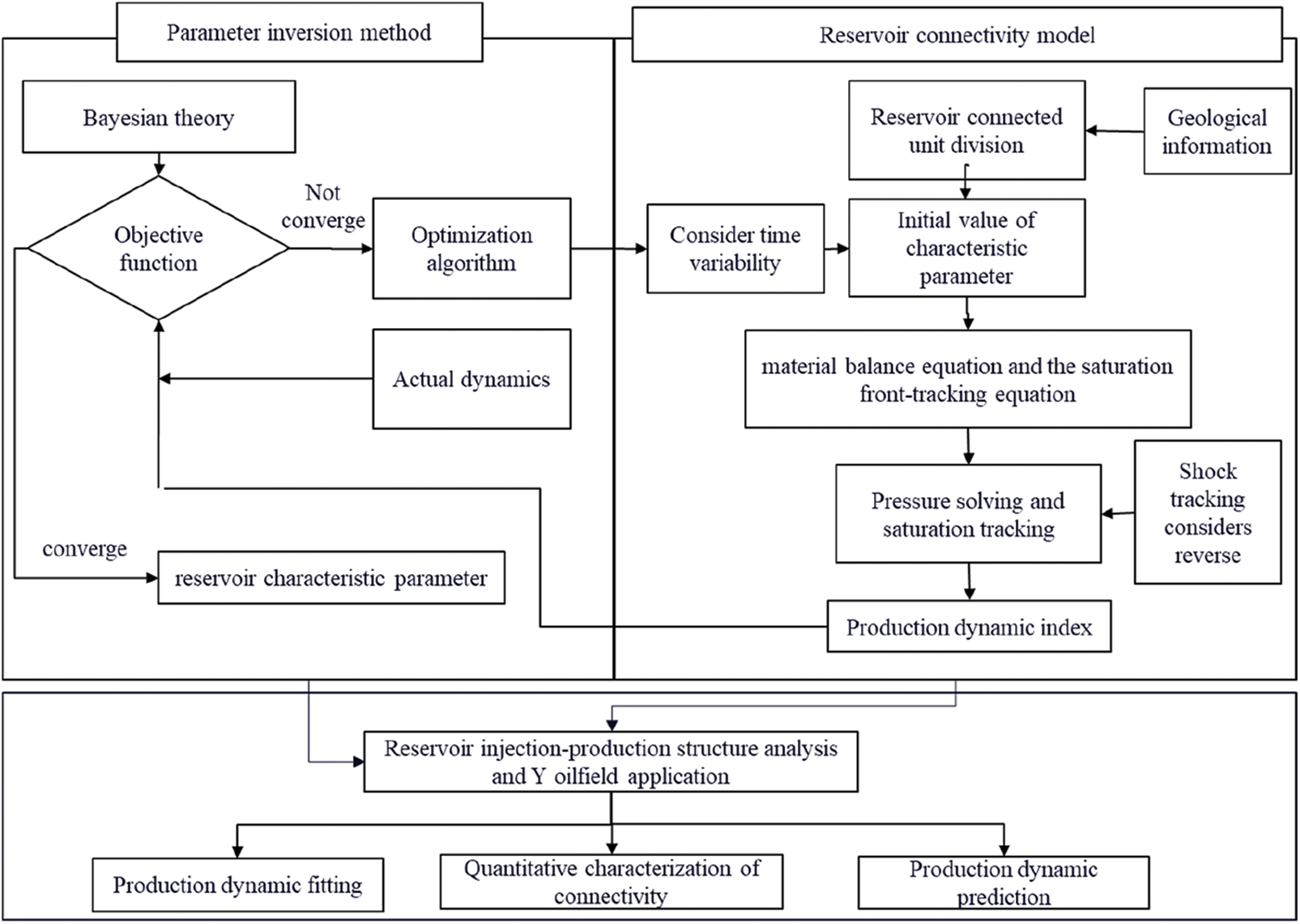
Figure 5: Technical roadmap of the thesis
A heterogeneous reservoir is constructed, and the three well patterns (1) one injection well and four production wells (one horizontal well, four vertical wells), (2) one production well and four injection wells (one horizontal well, four vertical wells), and (3) five production wells and four injection wells (all are horizontal wells), are used to validate the model. Based on the production performance and allocator of each well generated by The Eclipse numerical simulator the interwell connectivity model is established according to the above-mentioned method. The calculated production performance and the allocators are compared with the actual data to verify the model.
The grid of the reservoir is divided into 41 × 41 × 1 grids and the grid size in each direction is 10 m. The distribution of permeability is presented in Fig. 6, where the permeability unit is mD. The average porosity of the reservoir is 0.23, the initial irreducible water saturation is 0.28, and the initial formation pressure is 25 MPa. the viscosities of oil phase and water phase are 12.0 and 1.0 mPa⋅s, respectively. The reservoir well pattern is consisted of four vertical production wells and one horizontal injection well. The liquid production rate of well P1, P2, P3 and P4 is 25 m3/d, and the injection rate of well W1 is 100 m3/d. After 300 days of production, the production scheme is changed, the liquid production rates of wells P2 and P3 are increased to 40 m3/d, while the liquid production rates of wells P1 and P4 are reduced to 10 m3/d. The final water cut of the reservoir is 43.2% after 300 days of production.
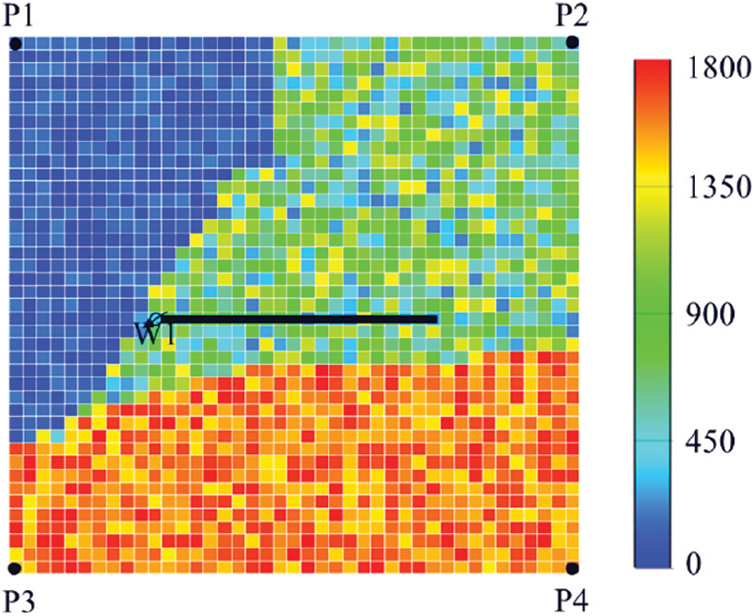
Figure 6: Reservoir permeability distribution
Both Eclipse model and connectivity model are used to match the historical oil production rate of single well and the cumulative oil production of the block. There are 100 iteration steps in total, and the change in objective function is shown in Fig. 7. The objective function converges after 10 iteration steps, and the total time required is 198 s.
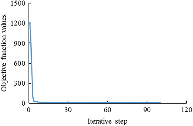
Figure 7: Iterative process of objective function
The fitting and prediction results are shown in Fig. 8. The block fitting rate reaches 99.5%, the fitting rate of well P1 reaches 97.0%, and the fitting rate of well P2 reaches 97.3%. The model fits well with the shistorical production dynamics and the prediction results also matched, which indicates the feasibility of this model to be applied to predict the future production performance.
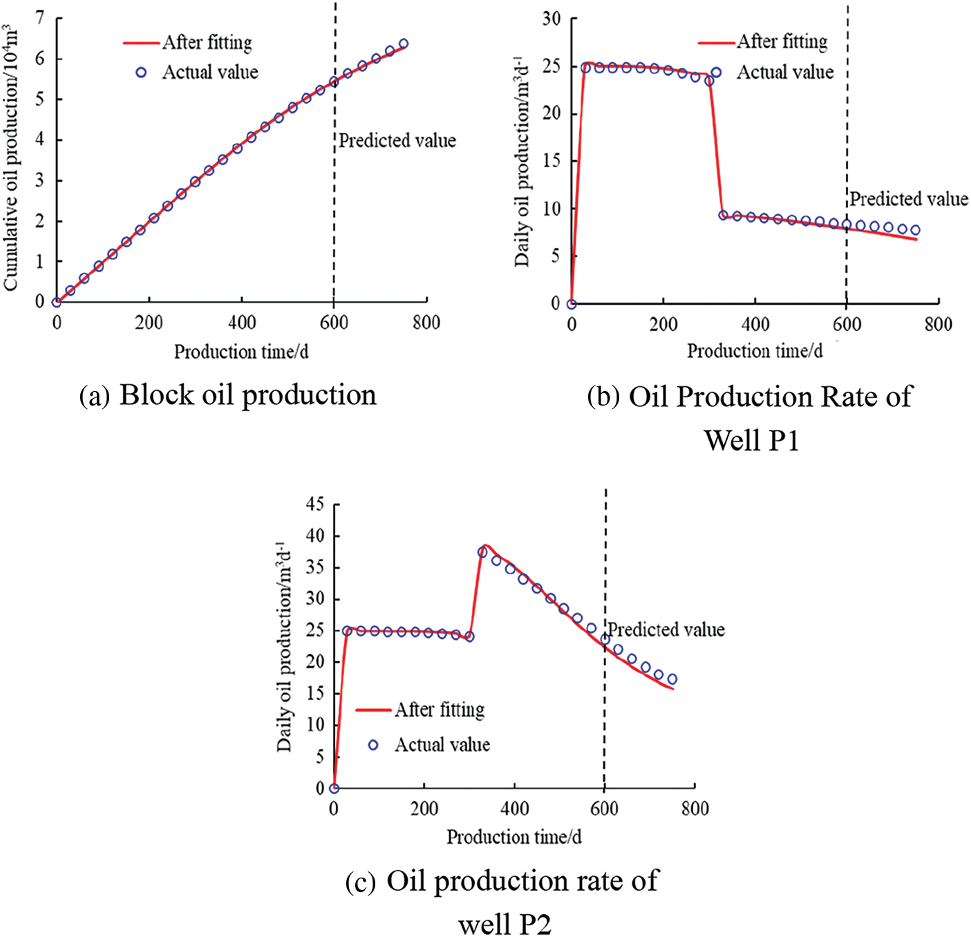
Figure 8: Production dynamic fitting and prediction results of single well and block
Fig. 9 is the distribution of conductivity and connected volume of the inversion model. It can be seen from the figure that the conductivity between P4 and W1 wells is high, and the permeability around P4 well is large from the permeability field distribution, which can be corresponded to the above. The conductivity between P2 and W1 is small. From the distribution of permeability field, it can be seen that the permeability around P2 is low and the heterogeneity is poor. The inversion results of this model are basically consistent with the physical properties input in the Eclipse model, which confirms the accuracy of this model.
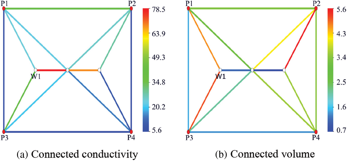
Figure 9: Parameter inversion results of connected elements
The connectivity model can also generate the injection/production allocators at different time intervals. Fig. 10 compares the water injection splitting values of the Eclipse model with the connectivity model, the results are very similar except for the allocator from W1 to P1 mainly because of the strong heterogeneity between the two wells. The physical point is included in this model, while the physical property distribution of the whole block is not neglected.
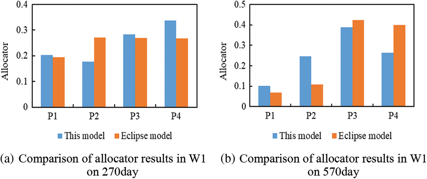
Figure 10: Results of water injection splitting comparison
Reservoir grid distribution and size are similar to Example one. But in this case, production wells and injection wells are switched. The current well pattern is composed of one horizontal production well and four vertical Injection wells, as shown in Fig. 6. The production rate of well P1 is 80 m3/d, and the injection rate for wells W1, W2, W3 and W4 are 20 m3/d. After 300 days of production, the production scheme is changed, the injection rate for wells W1 and W4 increases to 40 m3/d, while the injection rate for wells W2 and W3 declines to 10 m3/d, and the production rate of well P1 changes to 100 m3/d. The final water cut of the reservoir is 32.1% after 300 days of production.
Both Eclipse model and connectivity model are used to match the historical oil production rate of single well and the cumulative oil production of the block. There are 100 iteration steps in total, and the change in objective function is shown in Fig. 11. The objective function converges after 10 iteration steps, and the total time required is 209 s.
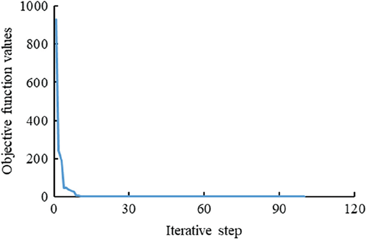
Figure 11: Iterative process of objective function
The fitting and prediction results are shown in Fig. 12. The block fitting rate reaches 99.9%, and the fitting rate of well P1 reaches 99.2%. The model fits well with the historical production dynamics and the prediction results also matched.
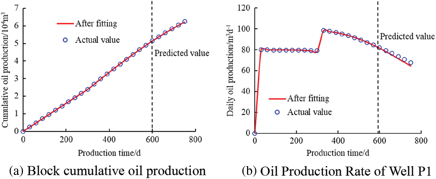
Figure 12: Production dynamic fitting and prediction results of single well and block
Fig. 13 is the distribution of conductivity and connected volume of the inversion model. It can be seen from the figure that the conductivity between P1 and W3 is high, and the permeability around W3 is large according to the permeability field distribution. The conductivity between P1 and W1 wells is low. From the permeability field distribution, it can be seen that the permeability around W1 well is small and the heterogeneity is poor. The inversion results of this model are basically consistent with the physical properties input in the Eclipse model.
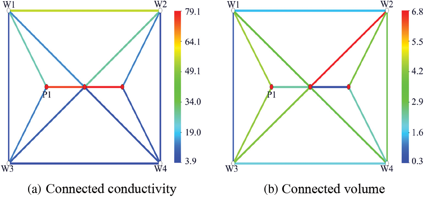
Figure 13: Parameter inversion results of connected elements
Fig. 14 compares the water inflow coefficients results of the Eclipse model with the connectivity model, the results are basically the same.
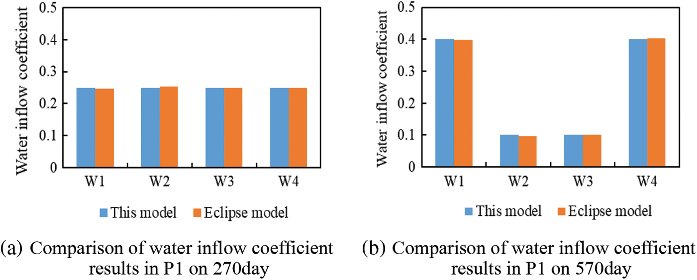
Figure 14: Comparison of water inflow coefficients
The grid of the reservoir model is divided into 81 × 41 × 1 grids, and The grid size for in each direction is 10 m. The interwell distances in the x Axis and y Axis directions are 100 and 200 m, respectively. The distribution of permeability is presented in Fig. 15, where the permeability unit is mD. Other physical property parameters remain the same with Example one. The reservoir well pattern is made up of five horizontal production wells and four horizontal injection wells. The liquid production rates of wells P1, P2, P3, P4 and P5 are 20 m3/d, and the injection rates of wells W1, W2, W3 and W4 are 25 m3/d. After 750 days of production, the production scheme is changed, the liquid production rates of wells P1 and P5 are increased to 30 m3/d, while the production rates of wells P2 and P4 are lowered to 20 m3/d, and the production rate of well P3 is maintained at 20 m3/d. The final water cut of the reservoir is 54.4% after 750 days of production.
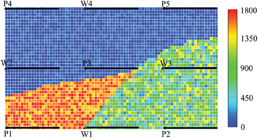
Figure 15: Reservoir permeability distribution
Both Eclipse model and connectivity model are used to match the historical oil production rate of single well and the cumulative oil production of the block. There are 100 iteration steps in total, and the change in objective function is shown in Fig. 16. The objective function converges after 80 iteration steps, and the total time required is 18459 s.
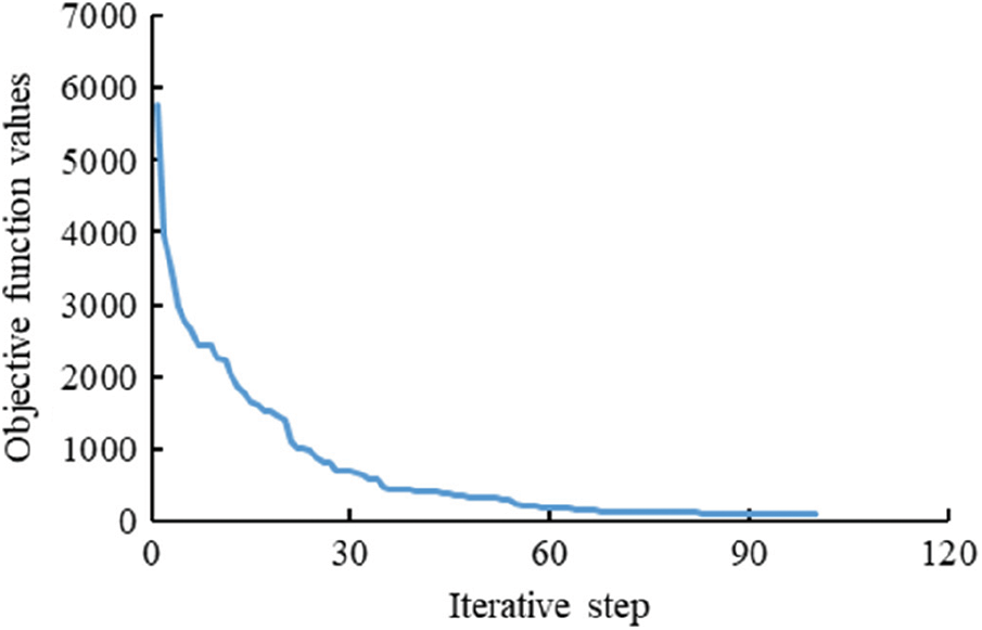
Figure 16: Iterative process of objective function
The fitting and prediction results are shown in Fig. 17. The block fitting rate reaches 99.7%, the fitting rate of well P1 reaches 94.6%, and the fitting rate of well P2 reaches 94.5%. The model fits well with the historical production dynamics and the prediction results also matched.

Figure 17: Production dynamic fitting and prediction results of single well and block
Fig. 18 is the distribution of conductivity and connected volume of the inversion model. It can be seen from the figure that the conductivity between P4 and W2 is high, and the permeability around P4 is large, which is close to that of W2. The conductivity between P2 and W3 wells is low, and the permeability around P2 well is low and the heterogeneity is poor. The poor heterogeneity between P3 and W1 leads to high permeability at the third node of P3 well and high conductivity at the third node of W1 well. The inversion results of this model are basically consistent with the physical properties input in the Eclipse model, which verifies the accuracy of the proposed model.


Figure 18: Parameter inversion results of connected elements
Fig. 19 compares the water injection splitting values of the Eclipse model with the connectivity model, the results are basically the same. The main reason for the incomplete coincidence of the results is that the model considers the physical properties of well points, while Eclipse considers the physical properties of all grid points.
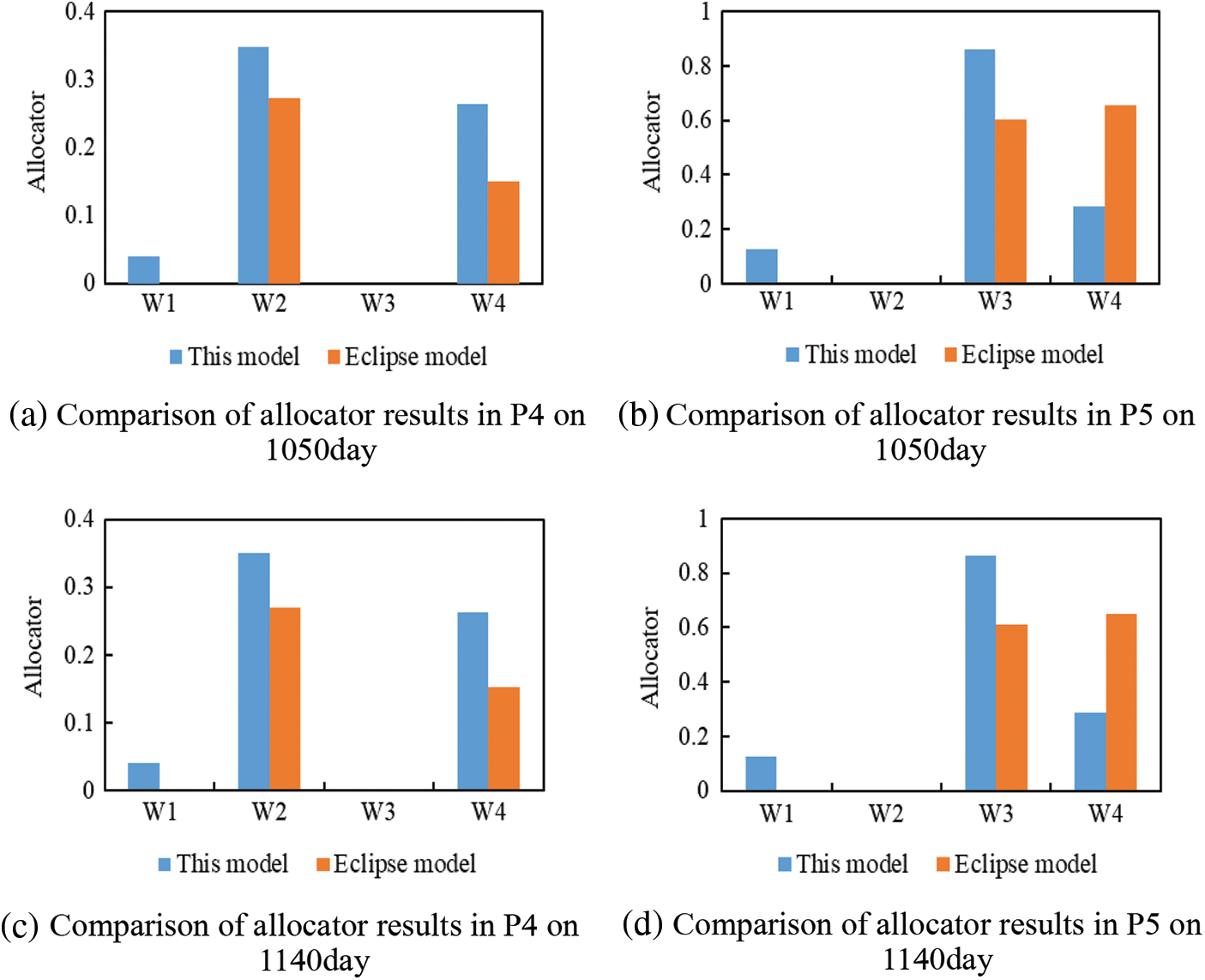
Figure 19: Comparison results of water injection allocator
The model is applied in the Block X of Y Oilfield and the well locations is shown in Fig. 20. The initial water saturation of this block is 0.376, the oil viscosity is 11.7 mPa⋅s, the water viscosity is 1.0 mPa⋅s, and the average porosity is 0.28. The distribution of reservoir thickness is shown in Fig. 21. There are 27 wells in total, which includes 16 production wells and 11 water injection wells, and 12 of them are horizontal wells (including production and injection wells). The proved reserves of the block is 8.393 × 10⁸m3. After 11 years production, the cumulative oil production, the oil recovery and the comprehensive water cut are 2.41 × 10⁸ m3, 28.7% and 88%, respectively with some wells entered into the water flooded stage.
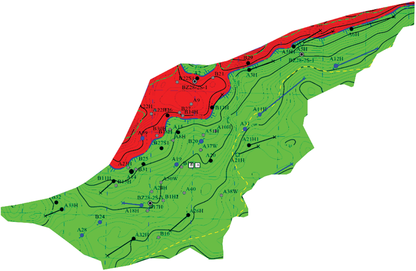
Figure 20: Well location distribution map of block X in Y oilfield
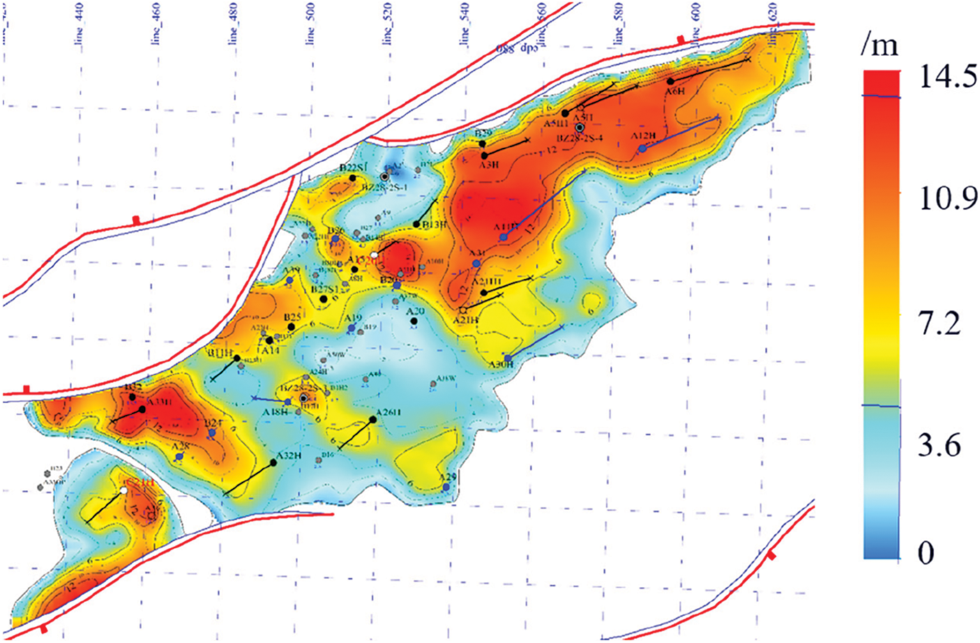
Figure 21: Information of reservoir thickness
SPSA method is used for production data matching, where the data includes oil production rate of a single well, water cut of a single well, cumulative oil production of block, and water cut of block. There are 250 iteration steps in total, and the change in objective function is shown in Fig. 22. The objective function converges after 200 iteration steps.
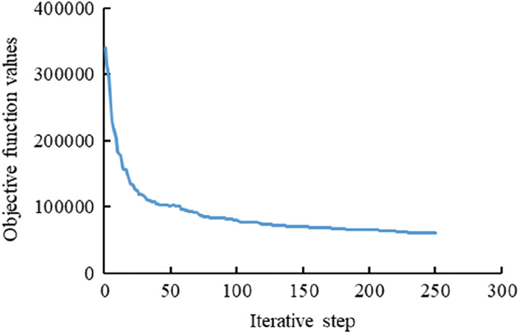
Figure 22: Iterative process of objective function
The fitting results of block cumulative oil production and oil production rates of some vertical well and horizontal wells are shown in Fig. 23. The inversion results of this model are basically consistent with the production dynamics, which confirms the accuracy of this model further.
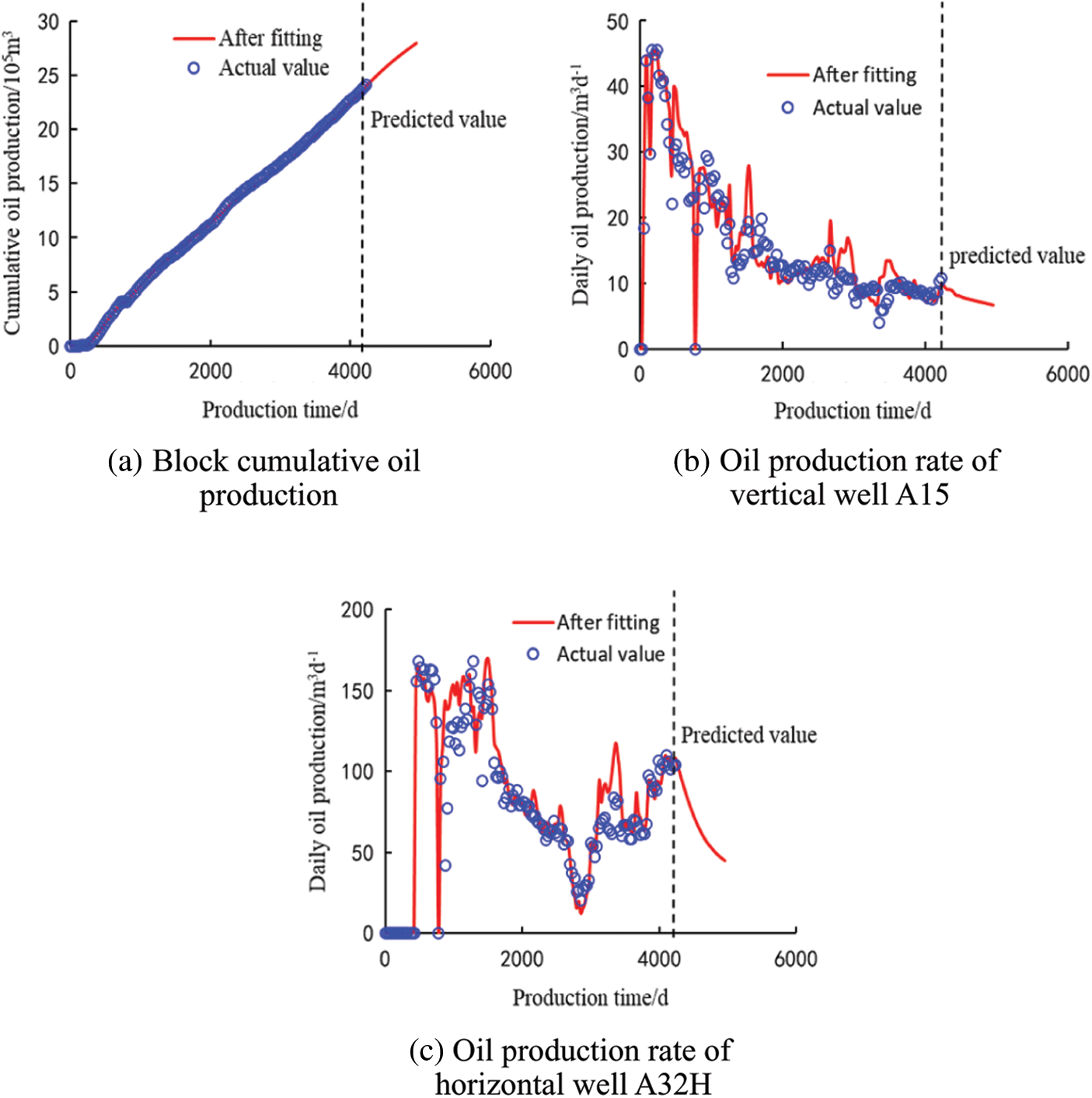
Figure 23: Production dynamic fitting of single well and block
Fig. 24 is the distribution of the average conductivity and connected volume of the inversion model for Block X of Y Oilfield. The results demonstrated that the conductivity between Well A6H and Well A12H, Well A5H1 and Well A12H, Well A33H and Well B24, Well A21H1 and Well A11H is higher than other well pairs. And the permeability of these well points is generally greater than the average reservoir permeability. The characteristic parameters such as interwell conductivity and connected volume can directly reflect the fluid flow in the reservoir, and can provide reliable data reference for the production dynamic analysis.

Figure 24: The inversion results of connectivity unit parameters in Block X of Y oilfield
Fig. 25 is water injection allocator for different time intervals obtained by inversion model. It can be seen from the figure that as for A11H well group on the 1260th day, A11H well mainly splits along the A6H well and A3H well directions with water injection allocators of 0.15 and 0.55, respectively. And on the 1290th day, the A11H well still mainly splits along the A6H well and the A3H well directions. By decreasing the liquid production rate of A3H and increasing the liquid production rate of A6H, the water injection allocator of A6H increases from 0.15 to 0.18 while the allocator of A3H decreases from 0.55 to 0.42 drop in the A3H well and the production of liquid lift in the A6H well, respectively, which indicates the good match between water injection allocators and actual production/injection dynamics, which is more efficient to the evaluate the water flooding effect.
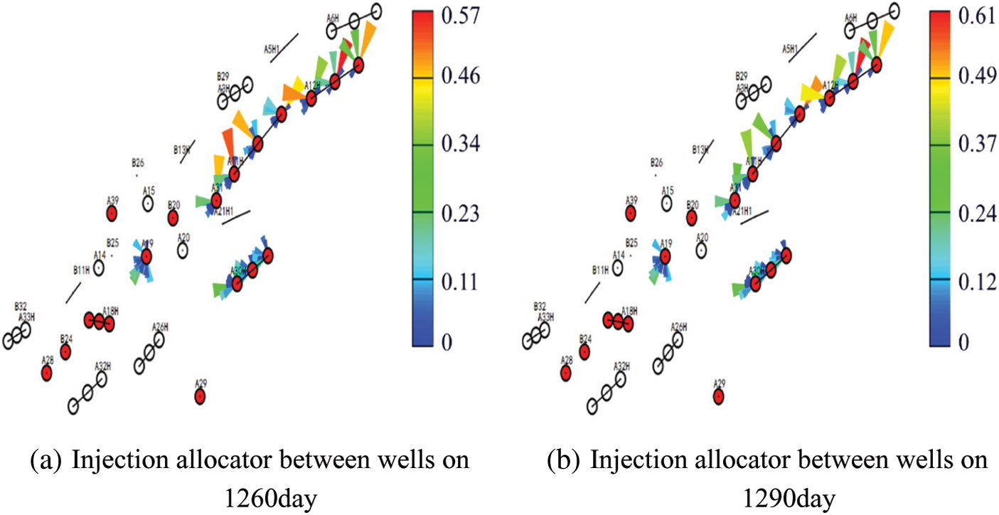
Figure 25: Water injection allocator between wells at different times in Block X of Y oilfield
(1) Horizontal wells are equivalently substituted by multiple connected nodes, and the injection-production system is equivalent to a connected network that can be characterized by parameters such as inter-well conductivity and connected volume. An injection-production connectivity model to study horizontal interwell connectivity in a water flooding reservoir is established, and a new calculation method to calculate production index is deduced. Based on the material balance equation and the shock wave tracing method, the saturation distribution of horizontal wells is calculated and the production dynamic of each well point is obtained. The SPSA algorithm is used to invert the interwell connectivity parameters and allocators on the basis of automatic history matching.
(2) The connectivity model is built based on injection/production data. Three typical examples, where the number ratio between injection and production wells are 1/4, 4/1 and 4/5, respectively, are used to fit the historical production performance and to make comparison with the results generated by the Eclipse, which verifies the effectiveness of the model.
(3) The Block X of Y Oilfield is used as an example, according to the injection/production data, the connectivity model is utilized to fit the historical production data. Meanwhile, the connectivity conductivity and volume for this model is inversed. The accuracy between the calculated cumulative oil production and the real values reaches 96.9%. According to the connectivity characteristics for typical well groups, the specific adjustment strategies are proposed and the practicability of the model is verified.
Acknowledgement: The authors would like to appreciate reviewers and editors whose critical comments were helpful in preparing this article.
Funding Statement: This study was supported by the National Natural Science Foundation of China (52004033, 51922007).
Conflicts of Interest: The authors declare that they have no conflicts of interest to report regarding the present study.
1. Feng, C. J., Bao, Z. D., Yang, L., Si, X., Xu, G. B. et al. (2014). Reservoir architecture and remaining oil distribution of deltaic front underwater distributary channel. Petroleum Exploration and Development, 41(3), 358–364. DOI 10.1016/s1876-3804(14)60040-9. [Google Scholar] [CrossRef]
2. Johnson, C. R., Greenkorn, R. A., Woods, E. G. (1966). Pulse-testing: A new method for describing reservoir flow properties between wells. Journal of Petroleum Technology, 18(12), 1599–1604. DOI 10.2118/1517-pa. [Google Scholar] [CrossRef]
3. Kamal, M., Bringham, W. E. (1975). Pulse testing response for unequal pulse and shut-in periods. SPE Journal, 15(5), 399–410. DOI 10.2118/5053-pa. [Google Scholar] [CrossRef]
4. Kang, Z. H., Chen, L., Lu, X. B., Yang, M. (2012). Fluid dynamic connectivity of karst carbonate reservoir with fracture & cave systemin tahe oilfield. Earth Science Frontiers, 19(2), 110–120. [Google Scholar]
5. Blasingame, T. A., Lee, W. J. (1986). Properties of homogeneous reservoirs, naturally fractured reservoirs, and hydraulically fractured reservoirs from decline curve analysis. SPE Permian Basin Oil and Gas Recovery ConferenceMidland, Texas, USA. DOI 10.2523/15018-ms. [Google Scholar] [CrossRef]
6. Blasingame, T. A., Lee, W. J. (1986). Variable-rate reservoir limits testing. SPE Permian Basin Oil and Gas Recovery ConferenceMidland, Texas, USA. DOI 10.2118/15028-ms. [Google Scholar] [CrossRef]
7. Zhang, Z., Chen, M. Q., Gao, Y. L. (2006). Estimation of the connectivity between oil wells and water injection wells in low-permeability reservoir using tracer detection technique. Journal of Xi’an Shiyou University, 21(3), 48–51. DOI 10.3969/j.issn.1673-064X.2006.03.013. [Google Scholar] [CrossRef]
8. Xu, H., Lin, C. Y., Zhang, Y. C., Jia, Z. Z. (2013). Numerical simulation of underwater distributary channel sand reservoir. Special oil & Gas Reservoirs, 20(4), 58–61. DOI 10.3969/j.issn.1006-6535.2013.04.014. [Google Scholar] [CrossRef]
9. Du, J., Yang, S. M. (2007). Analysis to the field application effect of inner well microseismic monitoring technique. Petroleum Geology & Oilfield Development in Daqing, 26(4), 120–122. DOI 10.3969/j.issn.1000-3754.2007.04.030. [Google Scholar] [CrossRef]
10. Xia, Z., Zhang, D. M., Kang, Z. J., Chen, D., Wang, M. (2016). A method for evaluating dynamic connectivity of dynamic injection production based on LMD and MLR model based on gauss evaluation. Geological Science and Technology Information, 35(6), 36–240. [Google Scholar]
11. Refunjol, B. T. (1996). Reservoir characterization of north buck draw field based on tracer response and production/injection analysis. Austin: University of Texas, Texas, USA. [Google Scholar]
12. Heffer, K. J., Fox, R. J., McGill, C. A., Koutsabeloulis, N. C. (1997). Novel techniques show links between reservoir flow directionality, earth stress, fault structure and geomechanical changes in mature waterfloods. SPE Journal, 2(2), 91–98. DOI 10.2118/30711-pa. [Google Scholar] [CrossRef]
13. Jansen, F. E., Kelkar, M. G. (1997). Non-stationary estimation of reservoir properties using production data. SPE Annual Technical Conference and ExhibitionSan Antonio, Texas, USA. DOI 10.2523/38729-ms. [Google Scholar] [CrossRef]
14. Panda, M. N., Chopra, A. K. (1998). An integrated approach to estimate well interactions. SPE India Oil and Gas Conference and ExhibitionNew Delhi, India. DOI 10.2118/39563-ms. [Google Scholar] [CrossRef]
15. Soeriawinata, T., Kelkar, M. (1999). Reservoir management using production data. SPE Mid-Continent Operations SymposiumOklahoma, USA. DOI 10.2118/52224-ms. [Google Scholar] [CrossRef]
16. Albertoni, A., Lake, L. W. (2003). Inferring interwell connectivity only from well-rate fluctuations in water floods. SPE Reservoir Evaluation and Engineering, 6(1), 16. DOI 10.2118/83381-pa. [Google Scholar] [CrossRef]
17. Dinh, A., Tiab, D. (2008). Inferring interwell connectivity from well bottomhole-pressure fluctuations in waterfloods. SPE Reservoir Evaluation and Engineering, 11(5), 874–881. DOI 10.2118/106881-pa. [Google Scholar] [CrossRef]
18. Dinh, A., Tiab, D. (2008). Interpretation of interwell connectivity tests in a waterflood system. SPE Annual Technical Conference and ExhibitionDenver, Colorado, USA. DOI 10.2118/116144-ms. [Google Scholar] [CrossRef]
19. Yousef, A. A., Jensen, J. L., Lake, L. W. (2006). Analysis and interpretation of interwell connectivity from production and injection rate fluctuation using a capacitance model. SPE Symposium on Improved Oil RecoveryTulsa, Oklahoma, USA, 92. DOI 10.2118/99998-ms. [Google Scholar] [CrossRef]
20. Yousef, A. A., Gentil, P. H., Jensen, J. L., Lake, L. W. (2006). A capacitance model to infer interwell connectivity from production and injection rate fluctuations. SPE Reservoir Evaluation and Engineering, 9(6), 30–646. DOI 10.2118/95322-ms. [Google Scholar] [CrossRef]
21. Lake, L. W., Liang, X., Edgar, T. F., Al-Yousef, A., Sayarpour, M. et al. (2007). Optimization of oil production based on a capacitance model of production and injection rates. SPE Hydrocarbon Economics and Evaluation SymposiumDallas, Texas, USA. DOI 10.2523/107713-ms. [Google Scholar] [CrossRef]
22. Sayarpour, M., Kabir, C. S., Lake, L. W. (2009). Field applications of capacitance-resistance models in waterfloods. SPE Reservoir Evaluation & Engineering, 12(6), 853–864. DOI 10.2118/114983-pa. [Google Scholar] [CrossRef]
23. Naudomsup, N., Lake, L. W. (2018). Extension of capacitance/Resistance model to tracer flow for determining reservoir properties. SPE Reservoir Evaluation & Engineering, 22(1), 266–281. DOI 10.2118/187410-pa. [Google Scholar] [CrossRef]
24. Nguyen, A. P., Kim, J. S., Lake, L. W., Edgar, T. F., Haynes, B. (2021). Integrated capacitance resistive model for reservoir characterization in primary and secondary recovery. SPE Annual Technical Conference and ExhibitionDenver, Colorado, USA. DOI 10.2118/147344-ms. [Google Scholar] [CrossRef]
25. Yousefi, S. H., Rashidi, F., Sharifi, M., Soroush, M., Ghahfarokhi, A. J. (2021). Interwell connectivity identification in immiscible gas-oil systems using statistical method and modified capacitance-resistance model: A comparative study. Journal of Petroleum Science and Engineering, 198, 108175. DOI 10.1016/j.petrol.2020.108175. [Google Scholar] [CrossRef]
26. Zhao, H., Kang, Z. J., Zhang, Y., Sun, H. T., Li, Y. (2014). An interwell connectivity numerical method for geological parameter characterization and oil-water two-phase dynamic prediction. Acta Petrolei Sinica, 35(5), 922–927. DOI 10.7623/syxb201405012. [Google Scholar] [CrossRef]
27. Zhao, H., Kang, Z. J., Zhang, X. S., Sun, H. T., Reynolds, A. C. (2016). A Physics-based data-driven numerical model for reservoir history matching and prediction with a field application. SPE Journal, 21(6), 2175–2194. DOI 10.2118/173213-pa. [Google Scholar] [CrossRef]
28. Zhao, H., Kang, Z. J., Zhang, X. S., Sun, H. T., Reynolds, A. C. (2016). A data-driven model for history matching and prediction. Journal of Petroleum Technology, 68(4), 81–82. DOI 10.2118/0416-0081-jpt. [Google Scholar] [CrossRef]
29. Guo, Z., Reynolds, A. C., Zhao, H. (2018). A Physics-based data-driven model for history matching, prediction, and characterization of waterflooding performance. SPE Journal, 23(2), 367–395. DOI 10.2118/182660-ms. [Google Scholar] [CrossRef]
30. Yao, S., Wang, X., Yuan, Q., Guo, Z., Zeng, F. (2020). Production analysis of multifractured horizontal wells with composite models: Influence of complex heterogeneity. Journal of Hydrology, 583, 124542. DOI 10.1016/j.jhydrol.2020.124542. [Google Scholar] [CrossRef]
31. Zhang, J. G. (2009). Oil and gas seepage mechanics. Dong’ying, China: University of Petroleum Press. [Google Scholar]
 | This work is licensed under a Creative Commons Attribution 4.0 International License, which permits unrestricted use, distribution, and reproduction in any medium, provided the original work is properly cited. |