| Fluid Dynamics & Materials Processing |
DOI: 10.32604/fdmp.2022.020942
ARTICLE
Prediction of Low-Permeability Reservoirs Performances Using Long and Short-Term Memory Machine Learning
School of Geosciences, Yangtze University, Wuhan, 430100, China
*Corresponding Author: Guowei Zhu. Email: changjiangshiyou1@163.com
Received: 21 December 2021; Accepted: 08 February 2022
Abstract: In order to overcome the typical limitations of numerical simulation methods used to estimate the production of low-permeability reservoirs, in this study, a new data-driven approach is proposed for the case of water-driven hypo-permeable reservoirs. In particular, given the bottlenecks of traditional recurrent neural networks in handling time series data, a neural network with long and short-term memory is used for such a purpose. This method can reduce the time required to solve a large number of partial differential equations. As such, it can therefore significantly improve the efficiency in predicting the needed production performances. Practical examples about water-driven hypotonic reservoirs are provided to demonstrate the correctness of the method and its ability to meet the requirements for practical reservoir applications.
Keywords: Water flooding; flow in porous media; data-driven; LSTM; CFD
Predicting well capacity in low-permeability reservoirs is a key part of field development management and the basis for optimally adjusting later development plans [1,2]. Oil field development is a complex system engineering task involving multiple scales, multiple physical fields, high nonlinearity, and several uncertainties. Therefore, production forecasting is a long-term problem and a difficult subject to master. In recent years, several researchers have investigated oil production using traditional methods such as petroleum reservoir engineering and numerical simulation of reservoirs [3,4].
In traditional reservoir design methods, the prediction of response time is mostly based on statistical production regimes. Only production or water injection data are used for reservoir production prediction. The accuracy of their estimation is low [5]. However, due to the limitations of the traditional numerical simulation methods for reservoirs. Only the flow field of porous media can be established according to physical rules. And due to factors such as grid shape, resolution, etc., lengthy dynamic simulation time is required. History matching is difficult. Therefore, there is a need for a prediction method for the development of water-driven low-permeability reservoirs that may increase efficiency and at the same time improve prediction accuracy [6].
Machine learning (ML) has grown in importance as artificial intelligence techniques have advanced over the past 20 years [7–9]. It is now widely used to study various subsurface and porous media models, especially in the oil exploration and production industries [10,11]. Especially in the oil exploration and production industry. ML techniques are also used in other sectors. Such as integrated re-observation and investigation of geological and environmental problems [12–14]. Forward neural networks (FNN), support vector machines (SVM), and radial basis functions (RBF) are capable of solving a wide range of complex problems and achieving the required prediction accuracy. However, when using such methods for point data prediction. It is often necessary to use different data rather than continuous data in order to make it valid (i.e., time series) [15]. In contrast to FNNs, recurrent neural networks (RNNs) have a “recursive” loop. This is a self-link from one node to its own time span. Thus, an implicit network is formed, which can be utilized to analyze inputs of any order. Moreover, information is propagated both backward and forward in the network. The RNN is allowed to teach at different time stages using backward transmission methods. This is referred to as learning “backward transmission”. Due to the presence of numerous backward transmission defects. On the other hand, gradients are no longer evident.
A deep learning based strategy was utilized in this study. Neural networks were used to predict long- and short-term memory neural networks for low-permeability oil field production [16]. By adding gating structures to a single self-loop structure. This approach replicates the signaling of real neurons, allowing the storage of longer-term sequential information [17]. Due to this advantage, LSTM has gained prominence in the discipline of artificial intelligence and deep learning. It has been used in various fields.Nelson and colleagues used LSTM networks to predict stock values based on historical and technical analysis data. With few exceptions, their results outperformed the baseline [18]. Zhao et al. [19] created a data-driven model, the LSTM-fully connected neural network to predict PM2.5 concentrations at a given air quality location by evaluating data from three sources: atmospheric quality data, meteorological data, and weather data. This strategy produces better prediction results compared to the findings of artificial neural network methods. LSTM can be used in combination with other deep learning methods, such as convolutional neural networks, to obtain greater results. Du et al. [20] proposed a technique based on convolutional resident LSTM to predict urban traffic flow. The technique is based on convolutional-resident LSTM. By merging LSTM cells with convolutional-resident network. The spatio-temporal characteristics of the multichannel matrix are investigated for the first time. The results show that this strategy largely outperforms existing DL-based prediction methods. Kamrava et al. [21] and colleagues used LSTM to predict complex matrices. All elements of this application show that LSTM performs well. It was shown to be able to extract not only dynamic changes from the data but also to represent correlations between time series.
This work uses deep LSTM models to predict crude oil production regimes in complex situations including low-permeability water-driven reservoirs, which are discussed in this paper. For greater clarity, we use data-driven techniques to address this problem. This avoids the need for additional flow simulations. The proposed model is able to predict the future trends of these variables based on their past patterns. Section 2 discusses RNNs and LSTMs, as well as their composition and mathematical formulation. For deep LSTM model building, Section 3 and Section 4 provide detailed methods and application examples, respectively. Section 5 summarizes the important findings in a concise manner.
2 Fundamental Principles and Methods
This section provides a quick introduction to the components and mechanism of RNN and LSTM, which may be used as a starting point for a more in-depth understanding of the suggested methodology.
It is suited for processing data having a temporal or sequential structure, as well as for processing data with different inputs and outputs. It has the capability of selectively sending information via sequential steps while processing sequential data one element at a time, as seen above. Acyclicity may be determined by unfolding the network as a deep neural network with one layer of time steps and weights that are shared across time steps. Furthermore, the hidden unit’s output containing stored information is sent to the hidden unit as part of its input at the next time step, which is then transferred back to the hidden unit. Nodes with cyclic edges receive input data points at the given time t, as well as hidden unit values h(t-1) from past states at the given time t. Without a doubt, such an action can efficiently preserve information from the previous stage in order to maintain track of the connections between data, hence improving the capacity to learn from and extract information from sequential data sets. The forward transfer in a basic RNN is mathematically regulated by the equation that follows (Fig. 1):
where
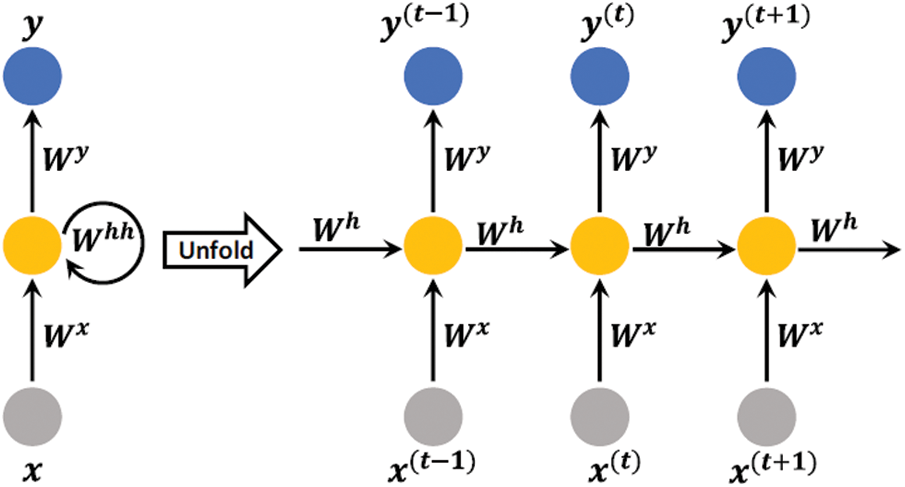
Figure 1: A simple unfolded RNN illustrated across time steps with one input unit, one hidden unit, and one output unit [22]
Although the structure of RNN allows information from previous steps to be continuously retained and influence the operation of subsequent steps, when the location of previous relevant information is very far away from the current computation step, the memory module (single tanh layer or sigmoid layer) in the model cannot effectively preserve the historical information for a long time due to the influence of constant input data and is prone to proble The memory module of an LSTM RNN differs from that of a normal RNN. LSTM can efficiently update and convey vital information in time series while successfully maintaining long-range information by applying a well-thought-out gate structure and memory unit state.Gates in the interaction layer can add, delete, and update information in the processor state using the hidden state from the previous step and the input from the current step, and the updated processor state and hidden state are transferred backward. The model can do single-factor prediction of a single indicator, multi-factor prediction of a single indicator, and multi-factor prediction of a single indicator in addition to end-to-end prediction. You can make predictions from start to finish using the LSTM model, and you can do single-factor prediction of a single indicator, multi-factor prediction of a single indicator, and multi-factor prediction of many indications all at once (Fig. 2).

Figure 2: LSTM model
The specific procedures of LSTM neural network at time step t are as follows:
(a) Decide what information should be discarded from the previous cell state Ct-1 in the forget gate ft.
(b) Identify what information of input xt should be stored into the cell state Ct in the input gate, where the input information it and the candidate cell state
(c) Update the cell state of the present time step Ct, which combine the candidate memory
(d) Confirm the outcome ht in the output gate where the output information ot and the cell state Ct is used.
A negative correlation between variables may be detrimental to the accuracy of model prediction in machine learning tasks. It is possible to reduce extraneous variables, increase model accuracy, and avoid the overmatching issue through the use of feature selection.
When it comes to feature selection approaches, recursive feature elimination is one of the most popular, and the basic concept is to utilize a base model (in this study, we use a support vector machine model) to undertake repeated training rounds. In the first step, training is carried out on all the features, and each feature is scored for the training outcome, as given in Eq. (1). The scoring procedure for each feature is also stated in Eq. (1). The features with the lowest scores, i.e., the ones that are considered to be the least relevant, are eliminated. The remaining features are utilized for the first round of training, and the procedure is repeated until just the final feature is left in the dataset. Because the order of feature elimination, i.e., the importance of the features, is such that the first feature eliminated is the least important and the last feature eliminated is the most important, the first feature eliminated is the least important and the last feature eliminated is the most important.
In order to improve the prediction accuracy of the model and eliminate the influence of the magnitude between the indicators, the input and output data need to be pre-processed. Since the data are more stable and there are no extreme maximum and minimum values, this paper adopts a normalization process to map them to the interval [0,1], and the linear transformation equation is:
where Xnorm represents the normalized data points inserted in the training process. Xold, Xmin and Xmax are the real values of the sample data and the lower and upper constraints of these real data corresponding to design variables or targets, respectively [23].
Production data from wells in water flooding low permeability reservoirs is often presented as a time-series of data. In addition, the LSTM neural network has adequate capability to perform good capacity prediction by first employing a long and short-term memory neural network for history matching before utilizing the LSTM neural network itself. Each time step during the history matching phase involves training the model with production series data as input characteristics and then comparing the results. At this point, only the production history of the first time step is known, and the expected production for the subsequent time step will be determined using the estimated values from the prior model, which will serve as the output of the previous model. To examine the error between the fitted data and the corresponding points of the original data, the sum squared error (SSE) is employed in this work. the sum squared error (SSE) is calculated by Eq. (7).
where Xexp represents the predicted value and Xhistory represents the true historical value. the closer the SSE is to 0, the better the model selection and fit, and the more successful the data prediction.
This paper presents an analysis of production data generated by a conventional numerical simulator, which is utilized to build a production forecast model. In this study, production data for a water flooding low-permeability block is used as experimental data for a total of 84 months, from January 2012 to December 2018. The training set, which contains data from January 2012 to December 2016, the validation set, which contains data from January 2017 to December 2017, and the test set, which contains data from January 2018 to December 2018, are the three datasets used.
For starters, the parameters of the LSTM neural network are randomly selected and initialized. In this example, the number of neural network layers is one, the time series step is twelve months, the number of neurons is forty, the number of network gates is forty-eight, and the number of training cycles is three thousand and one hundred. When that, the model is trained using the training data, and the model is prepared for validation after the training phase is done, as shown in the following diagram (Fig. 3).
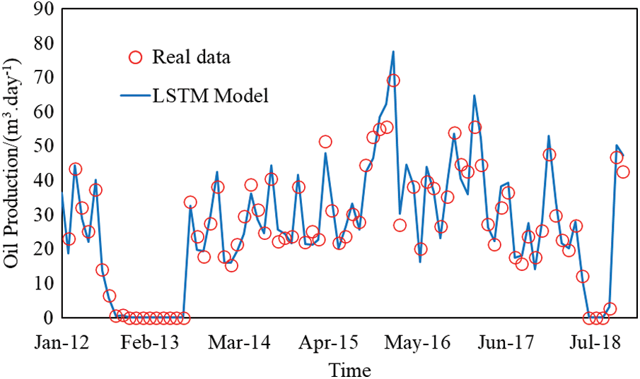
Figure 3: Matching of daily oil production rate of well A1
It was necessary to shut in the wells A1 and A2 in this block for a period of time in 2013. This was the point in time when the data was absent, the training samples were noisy, and the model was having some impact on the outcome. The prediction effect, on the other hand, is extremely good when the production is maintained indefinitely. When there are two consecutive switch-off wells, and the duration between the two switch-off wells is short, it can be observed that there is a big offset between the anticipated value and real value in this case, and the prediction is not very accurate. Predicted values and real values closely overlapped for the period from January 2014 to October 2017, and the prediction was more accurate in these circumstances.
The SSE of this training is depicted in Figs. 4 and 5. As the training cycle progresses, it can be seen that the SSE of this training lowers progressively. The final SSE is around 0.0005, which falls within a suitable error range and is within the acceptable error range for engineering applications, according to the results. In conclusion, the data-driven long and short term memory neural network reservoir simulation method can more accurately and quickly predict the future production dynamics of oil wells by fitting the production history more accurately and quickly, and the prediction accuracy meets the requirements of the mine site.

Figure 4: Matching of the daily oil production rate of well A2

Figure 5: SSE
The use of an LSTM-based prediction model to estimate the permeability of low-permeability reservoirs is proposed in this work. The model, which is based on data, allows engineers and decision-makers to obtain reservoir capacity information ahead of time, supporting them in developing low-permeability reservoir development plans that are better managed and regulated.
(1) It is possible to successfully fix the deficiencies of traditional reservoir engineering and reservoir numerical simulation approaches by utilizing a data-driven approach to low permeability reservoir production forecast, making it a helpful tool for reservoir development evaluation. (2) As a result, deep learning techniques are employed to train the model, which is based on the reservoir’s physical static property field as well as its dynamic production data, allowing it to achieve the goal of rapid reservoir development.
(2) When compared to conventional fully connected and conventional recurrent neural networks, the long and short-term memory neural network is a unique recurrent neural network that can better obtain information and perform the output of water flooding low-permeability oil fields than the other two types.
(3) According to the application findings of three algorithms, using long and short-term memory neural networks for oilfield production prediction is a good way. However, practical applications such as long-term prediction and parameter inversion still have significant limits, and future work will merge traditional reservoir numerical modeling with data-driven methods even more.
Funding Statement: The authors received no specific funding for this study.
Conflicts of Interest: The authors declare that they have no conflicts of interest to report regarding the present study.
1. Florence, F. A., Rushing, J., Newsham, K. E., Blasingame, T. A. (2007). Improved permeability prediction relations for low permeability sands. Rocky Mountain Oil & Gas Technology Symposium, Denver, Colorado, USA. DOI 10.2118/107954-MS. [Google Scholar] [CrossRef]
2. Sheikh, H. M. U. D., Lee, W., Jha, H., Ahmed, S. (2022). Establishing flow regimes for multi-fractured horizontal wells in lowpermeability reservoirs. International Petroleum Technology Conference and Exhibition, Dharan, Saudi Arabia. DOI 10.2535/IPTC-22694-MS. [Google Scholar] [CrossRef]
3. Li, H., Li, Y., Chen, S., Guo, J., Wang, K. et al. (2016). Effects of chemical additives on dynamic capillary pressure during waterflooding in low permeability reservoirs. Energy Fuels, 30(9), 7082–7093. DOI 10.1021/acs.energyfuels.6b01272. [Google Scholar]
4. Alhuraishawy, A. K., Bai, B., Wei, M., Geng, J., Pu, J. (2018). Mineral dissolution and fine migration effect on oil recovery factor by low-salinity water flooding in low-permeability sandstone reservoir. Fuel, 220, 898–907. DOI 10.1016/j.fuel.2018.02.016. [Google Scholar] [CrossRef]
5. Xu, Y., Sheng, G., Zhao, H., Hui, Y., Zhou, Y. et al. (2021). A new approach for gas-water flow simulation in multi-fractured horizontal wells of shale gas reservoirs. Journal of Petroleum Science Engineering, 199, 108292. DOI 10.1016/j.petrol.2020.108292. [Google Scholar] [CrossRef]
6. Xu, Y., Hu, Y., Rao, X., Zhao, H., Zhong, X. et al. (2021). A fractal physics-based data-driven model for water-flooding reservoir (FlowNet-fractal). Journal of Petroleum Science Engineering, 210, 109960. DOI 10.1016/j.petrol.2021.109960. [Google Scholar] [CrossRef]
7. Abhilash, E., Joseph, M. A., Krishna, P. (2006). Prediction of dendritic parameters and macro hardness variation in permanent mould casting of Al-12%Si Alloys Using Artificial Neural Networks. Micro-Structure Simulation, 2(3), 211–220. [Google Scholar]
8. Shamsa, A., Paydayesh, M., Faskhoodi, M. (2022). Bridging the gap between domain and data science; Explaining model prediction using SHAP in Duvernay field. Second EAGE Digitalization Conference and Exhibition, pp. 1–5. European Association of Geoscientists & Engineers. DOI 10.3997/2214-4609.202239056. [Google Scholar] [CrossRef]
9. Parra, J. O. (2022). Deep learning for predicting permeability logs in offset wells using an artificial neural network at a Waggoner Ranch reservoir, Texas. Leading Edge, 41(3), 184–191. DOI 10.1190/tle41030184.1. [Google Scholar] [CrossRef]
10. Kamali, M. Z., Davoodi, S., Ghorbani, H., Wood, D. A., Mohamadian, N. et al. (2022). Permeability prediction of heterogeneous carbonate gas condensate reservoirs applying group method of data handling. Marine Petroleum Geology, 105597. DOI 10.1016/j.marpetgeo.2022.105597. [Google Scholar] [CrossRef]
11. Jha, H. S., Khanal, A., Lee, J. (2022). Statistical and machine-learning methods automate multi-segment Arps decline model workflow to forecast production in unconventional reservoirs. SPE Canadian Energy Technology Conference, Calgary, Alberta, Canada. DOI 10.2118/208884-MS. [Google Scholar] [CrossRef]
12. Crnkovic-Friis, L., Erlandson, M. (2015). Geology driven EUR prediction using deep learning. SPE Annual Technical Conference and Exhibition, Houston, Texas, USA. DOI 10.2118/174799-MS. [Google Scholar] [CrossRef]
13. Mehta, A. (2016). Tapping the value from big data analytics. Journal of Petroleum Technology, 68(12), 40–41. DOI 10.2118/1216-0040-JPT. [Google Scholar] [CrossRef]
14. Li, H., Misra, S. (2018). Long short-term memory and variational autoencoder with convolutional neural networks for generating NMR T2 distributions. IEEE Geoscience Remote Sensing Letters, 16(2), 192–195. DOI 10.1109/LGRS.2018.2872356. [Google Scholar] [CrossRef]
15. Zhou, Y., Xu, Y., Rao, X., Hu, Y., Liu, D. et al. (2021). Artificial Neural Network-(ANN-) based proxy model for fast performances’ forecast and inverse schedule design of steam-flooding reservoirs. Mathematical Problems in Engineering, 2021(4), 1–12. DOI 10.1155/2021/5527259. [Google Scholar] [CrossRef]
16. Wang, H. L., Mu, L. X., Shi, F. G., Dou, H. E. (2020). Production prediction at ultra-high water cut stage via Recurrent Neural Network. Petroleum Exploration Development, 47(5), 1084–1090. DOI 10.1016/S1876-3804(20)60119-7. [Google Scholar] [CrossRef]
17. Hochreiter, S., Schmidhuber, J. (1997). Long short-term memory. Neural Computation, 9(8), 1735–1780. DOI 10.1162/neco.1997.9.8.1735. [Google Scholar] [CrossRef]
18. Nelson, D. M., Pereira, A. C., de Oliveira, R. A. (2017). Stock market’s price movement prediction with LSTM neural networks. International Joint Conference on Neural Networks, pp. 1419–1426. IEEE Anchorage, AK, USA. [Google Scholar]
19. Zhao, J., Deng, F., Cai, Y., Chen, J. (2019). Long short-term memory-Fully connected (LSTM-FC) neural network for PM2.5 concentration prediction. Chemosphere, 220, 486–492. DOI 10.1016/j.chemosphere.2018.12.128. [Google Scholar] [CrossRef]
20. Du, B., Peng, H., Wang, S., Bhuiyan, M. Z. A., Wang, L. et al. (2019). Deep irregular convolutional residual LSTM for urban traffic passenger flows prediction. IEEE Transactions on Intelligent Transportation Systems, 21(3), 972–985. DOI 10.1109/TITS.2019.2900481. [Google Scholar] [CrossRef]
21. Kamrava, S., Tahmasebi, P., Sahimi, M., Arbabi, S. (2020). Phase transitions, percolation, fracture of materials, and deep learning. Physical Review E, 102(1), 011001. DOI 10.1103/PhysRevE.102.011001. [Google Scholar] [CrossRef]
22. Bai, T., Tahmasebi, P. (2021). Efficient and data-driven prediction of water breakthrough in subsurface systems using deep long short-term memory machine learning. Computational Geosciences, 25(1), 285–297. DOI 10.1007/s10596-020-10005-2. [Google Scholar] [CrossRef]
23. Song, X., Liu, Y., Xue, L., Wang, J., Zhang, J. et al. (2020). Time-series well performance prediction based on Long Short-Term Memory (LSTM) neural network model. Journal of Petroleum Science Engineering, 186(2), 106682. DOI 10.1016/j.petrol.2019.106682. [Google Scholar] [CrossRef]
 | This work is licensed under a Creative Commons Attribution 4.0 International License, which permits unrestricted use, distribution, and reproduction in any medium, provided the original work is properly cited. |