| Fluid Dynamics & Materials Processing |
DOI: 10.32604/fdmp.2022.020271
ARTICLE
Experimental Study and Numerical Simulation of Polymer Flooding
1Xinjiang Oilfield Company, PetroChina (Experimental Testing Research Institute), Karamay, 834000, China
2Xinjiang Conglomerate Reservoir Laboratory, Karamay, 834000, China
3School of Petroleum Engineering, Yangtze University, Wuhan, 430100, China
*Corresponding Author: Kai Li. Email: lkll2014@petrochina.com.cn
Received: 14 November 2021; Accepted: 08 March 2022
Abstract: The numerical simulation of polymer flooding is a complex task as this process involves complex physical and chemical reactions, and multiple sets of characteristic parameters are required to properly set the simulation. At present, such characteristic parameters are mainly obtained by empirical methods, which typically result in relatively large errors. By analyzing experimentally polymer adsorption, permeability decline, inaccessible pore volume, viscosity-concentration relationship, and rheology, in this study, a conversion equation is provided to convert the experimental data into the parameters needed for the numerical simulation. Some examples are provided to demonstrate the reliability of the proposed approach.
Keywords: Polymer flooding; oil displacement mechanism; flooding experiment; numerical simulation; characteristic parameter
Nomenclature
| R | Retention of polymer in rock core, μg/g; |
| C0 | Concentration of injected polymer solution, mg/L; |
| V0 | Cumulative volume of polymer solution injected, mL; |
| Ci | Polymer concentration of the ith outflow sample at the core outlet, mg/L; |
| Vi | Volume of the ith outflow sample at the core outlet end, mL; |
| w | Dry core mass, g; |
| Ad istars | Adsorption capacity of component i, gmol/cm3; |
| Ad ilab | Measured adsorption capacity, mg/100 g; |
| ρr | Rock density, g/cm3; |
| ϕ | Porosity, %; |
| tad1 | The first parameter in Langmuir’s expression, gmol/cm3; |
| tad2 | The second parameter in Langmuir’s expression is related to mineralization, gmol/cm3; |
| tad3 | The third parameter in Langmuir’s expression, %; |
| xnacl | Salinity of salt, %; |
| ci | Mole fraction of component i, %; |
| ADMAXT | Cumulative adsorption capacity of polymer in unit volume rock, gmol/cm3; |
| △Pa | Differential pressure of water flooding, MPa; |
| △Pb | Differential pressure of polymer flooding, MPa; |
| △Pp | Differential pressure of subsequent water flooding MPa; |
| K | Permeability, mD; |
| μ | Viscosity, mPa⋅s; |
| RF | Resistance factor; |
| RRF | Residual resistance factor; |
| Rkα | α Phase permeability reduction factor; |
| Adcell | Adsorption capacity in grid, gmol/cm3; |
| kefα | α Phase effective permeability; |
| kabs | Absolute permeability of rock; |
| krα | α Phase relative permeability; |
| IPV | Inaccessible pore volume coefficient; |
| PV | Multiple of injected pore volume; |
| Vr | Volume of residual polymer solution in core, mL; |
| wp | Mole (or mass) fraction of key components; |
| wi | Mole (or mass) fraction of aqueous phase; |
| f(wp) | A mixing function corresponding to any component wp; |
| μaq | Aqueous viscosity, mPa⋅s; |
| μp | Pure component viscosity, mPa⋅s; |
| μw | Viscosity of water components, mPa⋅s; |
| μi | Viscosity of component I, mPa⋅s; |
| | Number of non-critical components in liquid phase; |
| Ul | Darcy rate, cm/s; |
| γfac | Shear rate, 1/s; |
| Sl | Saturation; |
| n | Shear thinning index factor; |
| C | Constant, related to the bending degree of porous media. |
Polymer flooding is widely used in various oil fields, which greatly improves the development effect of water flooding reservoirs. Research results have shown that the geological reserves suitable for polymer flooding are 29.10 × 10⁸ t, which can improve the oil recovery rate by 9.7% and increase recoverable reserves by 2.81 × 10⁸ t [1]. By the end of 2015, the cumulative produced reserves of polymer flooding had reached about 10 × 108 t, and enhanced oil recovery (EOR) was about 12.5% [2]. At present, polymer flooding or compound flooding field tests and applications have been carried out in Daqing, Shengli, Henan, Xinjiang, Dagang, Liaohe, and Bohai Oilfields, all of which have shown significant oil increasing effects [3–6].
With the large-scale industrial application of polymer flooding, the understanding of polymer flooding mechanism is deepening, and higher requirements have been proposed for the numerical simulation accuracy of polymer flooding mechanism and physicochemical phenomena. To reflect the physicochemical process of polymer flooding in the numerical simulation model, it is necessary to input multiple sets of characteristic parameters into the simulator, and the rationality of parameters affects the accuracy of the simulation results. At present, the characteristic parameters are tested mainly by experience and experimental methods, which usually have large errors. The ability to obtain specific physical and chemical characteristic parameters through experimental methods and to ensure the rationality of parameter settings is a bottleneck in the current development of polymer flooding reservoir numerical simulation technology.
In this study, through the analysis of polymer flooding mechanism and physicochemical phenomena, and combined with the characteristic parameters required by the CMG STARS reservoir numerical simulator, we selected the Karamay conglomerate reservoir as the research object. We conducted a core flooding experiment and used the CMG simulator to carry out a numerical simulation inversion of the physical model experiment. We verified the reliability and accuracy of the physical model experiment and provided a reference basis for the selection of polymer characteristic parameters.
2 Main Physicochemical Parameters and Experimental Results of Polymer Flooding
2.1 Main Physicochemical Parameters of Polymer Flooding
When the polymer is injected into the reservoir, the porous media in the reservoir retains the flowing polymer on its surface, which is the adsorption of the polymer [7]. Through a polymer flooding experiment, we took one sample per 2 mL of polymer solution at the outlet end. We measured the change in functional group concentration, injection amount, and recovery amount according to the starch chromium iodide method. The retention amount of the polymer in the formation is calculated by the material balance method, as follows:
In the numerical simulation of chemical flooding reservoir, the adsorption capacity in each grid needs to be calculated according to the chemical agent concentration dynamic adsorption retention data table or the Langmuir isothermal adsorption model.
The formula for converting data to reservoir digital analog data is as follows:
The index reflecting the ability of a polymer solution to reduce the permeability of porous media is called the residual resistance factor (RRF) [8,9]. Through the polymer flooding experiment, we successively measured the differential pressure ΔPa, ΔPp, and ΔPb of water flooding, polymer flooding, and subsequent water flooding at the same injection rate and calculated the resistance factor and RRF. The relationship between RRF and permeability was clarified, as follows:
The adsorption of polymers, especially those caused by chemical or mechanical (retention) types, will cause changes in permeability. The simulator simulates this process through RRF:
With an increase in adsorption capacity, Rkα changes from 1 to
2.1.3 Inaccessible Pore Volume
When macromolecular polymers flow through porous media, only water or salt may pass through a small part of pores; this part of pore volume is called the inaccessible pore volume [10].
Through the polymer flooding experiment, we collected the polymer solution at the outlet end and measured the concentration of the polymer sample until the polymer concentration in the outlet fluid was the same as the initial concentration. Inaccessible pore volumes can be calculated according to the following method:
The accessible pore volume is represented by *PORFT in the numerical simulation of chemical flooding reservoir, and the value of (1 − IPV) is the accessible pore volume.
2.1.4 Viscosity-Concentration Relationship
Polymer solution viscosity varies with concentration. The CMG STARS simulator (Computer Modelling Group, Ltd., Alberta, Canada) adopts the nonlinear viscosity calculation model. We fitted the coefficients of the nonlinear concentration calculation model through the concentration and viscosity data of the polymer solution.
The method of regression of polymer viscosity-concentration curve is as follows:
The rheology of a polymer solution refers to the relationship between viscosity and flow velocity when the polymer solution flows through a porous media under the action of an external force [11,12].
We directly used the experimental data for digital simulation. If the experimental data or simple power-law relationship were not sufficient, the relationship between rate viscosity or shear rate viscosity could be applied as follows:
Moreover, the viscosity of pure components can be calculated using the nonlinear mixing model:
2.2 Experimental Results of Polymer Flooding Characteristic Parameters
The polymer resistance factor, RRF, retention, inaccessible pore volume, viscosity-concentration, and rheological parameters are shown in Table 1, Figs. 1 and 2.
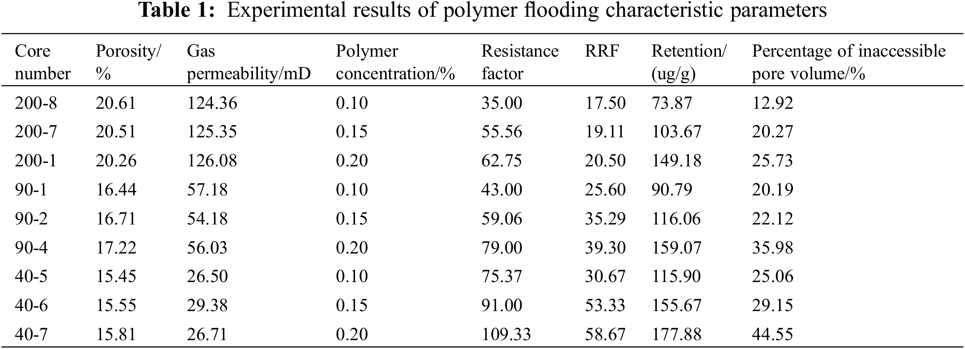
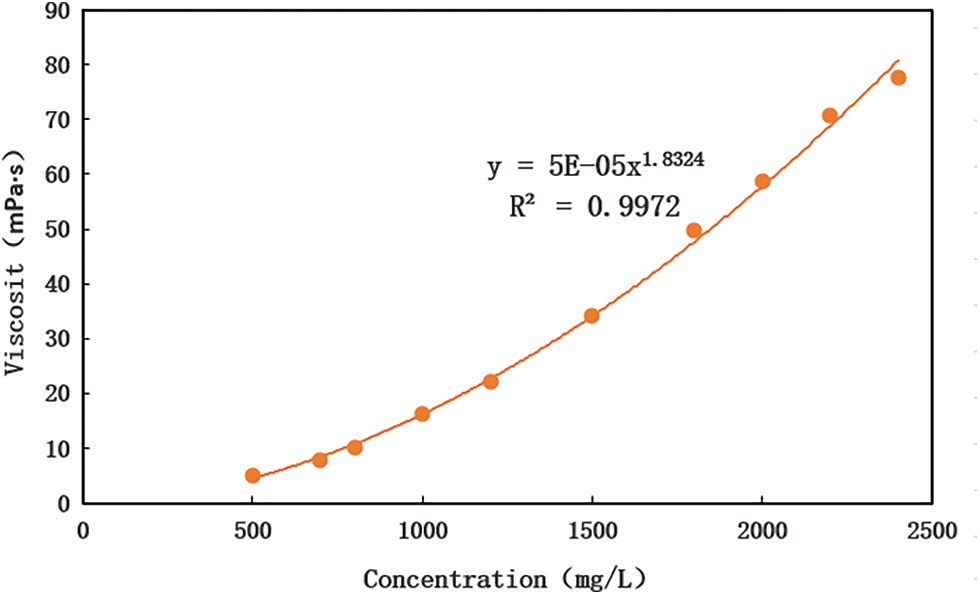
Figure 1: Viscosity-concentration diagram of polymer solution
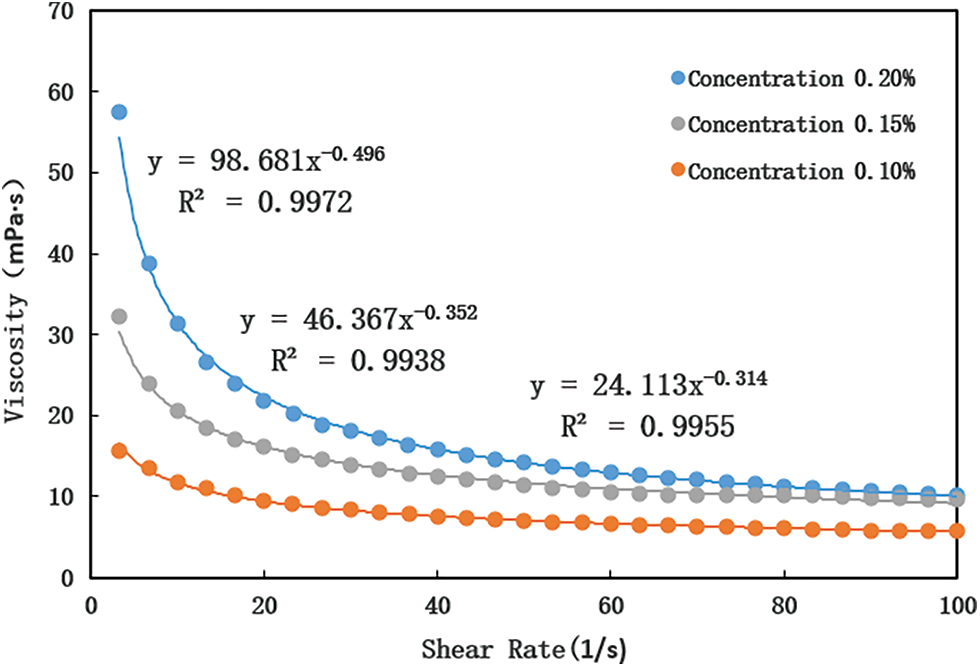
Figure 2: Viscosity-shear rate diagram of polymer solution
Fig. 1 shows that the viscosity-concentration relationship of a polymer solution was a power function and that the viscosity increased with the increase of concentration.
Fig. 2 shows that the viscosity of polymer solution gradually decreased with an increase in shear rate. When the shear rate increased to a certain extent, the viscosity tended to a constant value.
As shown in Table 1, under the same permeability conditions, with an increase in the polymer concentration, the resistance factor, RRF, retention, and inaccessible pore volume increased. With the increase of polymer concentration, the viscosity of the polymer solution increased. It first increased the viscous force of the displacement phase and further increased the flow resistance of the polymer solution. Then, it became more difficult for polymer molecules to enter the smaller pore throat. In addition, the polymer solution with a higher mass concentration had a stronger diffusion and dispersion effect. More polymer molecules were diffused into the transition zone of the displacement front, which resulted in more polymer molecules in the solid area of the core under the same permeability.
Moreover, at the same concentration, with a decrease in permeability, the resistance factor, RRF, retention, and inaccessible pore volume increased. Note that the lower the permeability of the core, the smaller the average pore throat radius and the greater the flow resistance, which both made it difficult for the macromolecules in the polymer solution to pass through and increased the inaccessible pore volume. In addition, the lower the permeability of the core with the same volume, the larger the internal solid surface area, which increased the number of solid surface adsorption points and caused more polymer molecules to be adsorbed inside the core, thus resulting in large adsorption retention.
Experimental equipment included a core gripper, a constant speed and pressure pump, and a constant temperature oven, as shown in Fig. 3.
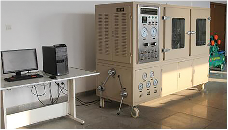
Figure 3: Polymer flooding experimental device
Experimental materials included artificial cores, crude oil, polymers, and simulated formation water. The core diameter and length were about 2.5 and 10 cm, respectively. The crude oil was degassed and dehydrated, and its viscosity was 15.3 mPa⋅s at 40°C. The polymer was polyacrylamide with an average relative molecular mass of 15 million. We configured a polymer solution with a mass concentration of 2000 mg/L. The brine contained 10.0001 g of sodium chloride (NaCl), 0.2153 g of magnesium sulfate heptahydrate (MgSO4⋅7H2O), 0.4163 g of anhydrous calcium chloride (CaCl2), and 2.8243 g of sodium bicarbonate (NaHCO3) per 1000 g of solution.
Following are the experimental steps:
1. Preparation of chemical agent: we prepared the required polymer solution (0.15%) with simulated formation water, transferred it into an intermediate container, and placed it in a constant temperature oven.
2. Saturate the core and measure the initial water phase permeability: after the rock core was cut, cleaned, and dried, we measured its porosity and permeability and loaded it into the core holder. After more than 4 h of evacuation, we used the simulated formation water to saturate the core and measured the pore volume (Vp). Then, we measured the displacement pressure difference (ΔP1) of the water sample at a fixed displacement speed of 0.2 mL/min by using a constant speed and constant pressure pump and calculated the water phase permeability (Kw1).
3. Establish irreducible water and measure oil phase permeability: first, we established irreducible water by oil displacement, then conducted displacement at the speed of 0.2 mL/min, recorded the displacement pressure difference (ΔP2) when it was stable, and calculated the oil phase permeability (Ko) under irreducible water.
4. Water flooding: we used simulated formation water to drive oil at the rate of 0.2 mL/min, recorded the pressure at the inlet end of the core and the water and oil production at the outlet end at different times, recorded the data every 10 min in the early stage, and recorded the data every 30 min when the oil content at the outlet was very small until the water cut reached 100% and the pressure was stable. Then, we recorded the oil production V1 and the displacement pressure difference (ΔP3), and we calculated the recovery factor, residual oil saturation, and water phase permeability at residual oil saturation (Kw2).
5. Polymer flooding: we set the pump to inject the polymer solution into the core at a constant flow rate of 0.2 mL/min, recorded the pressure and oil recovery at the inlet end of the core until the pressure was stable, recorded the oil recovery (V2) and the displacement pressure difference (ΔP4), and calculated the chemical flooding permeability (Kh) and oil recovery.
6. Subsequent water flooding: we set the pump to inject the polymer solution into the core at a constant flow rate of 0.2 mL/min, recorded the pressure at the inlet end of the core, and collected the polymer solution at the outlet end until the pressure was stable. Then, we recorded the displacement pressure difference (ΔP5) and calculated the water permeability (Kw3).
The relative permeability curve and the experimental results of polymer flooding are illustrated in Figs. 4 and 5, respectively.
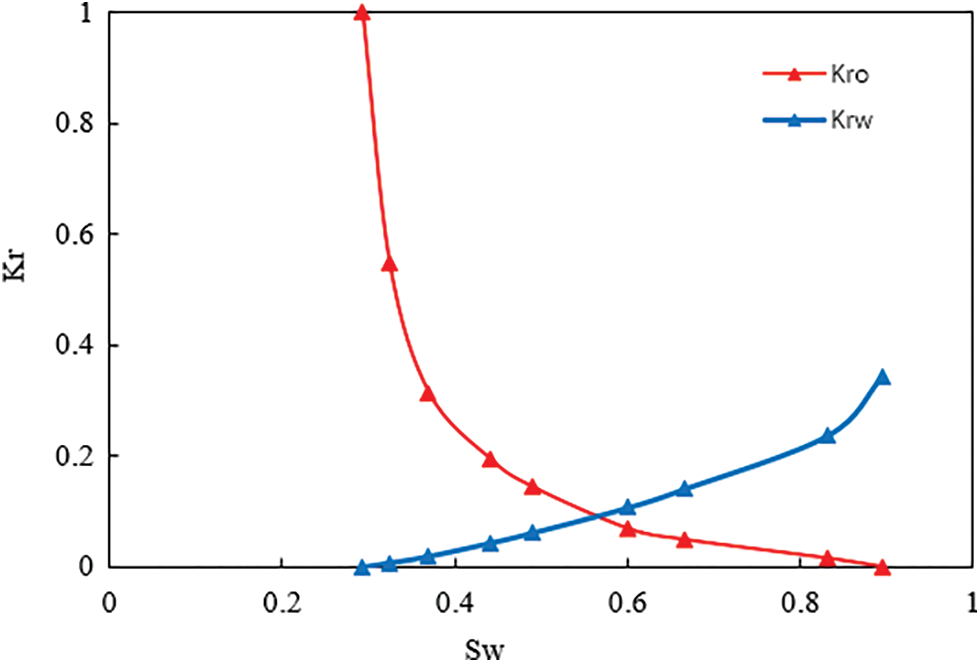
Figure 4: Relative permeability curve
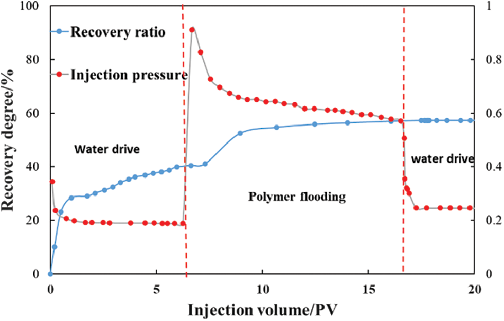
Figure 5: Experimental results of polymer flooding
Fig. 5 shows that the recovery degree increased by 18.18% after polymer flooding, and the final total oil displacement efficiency reached 59.20%. The water cut decreased at the initial stage of polymer injection, which indicated that the polymer had a good effect of profile control and displacement.
4 Numerical Simulation Inversion
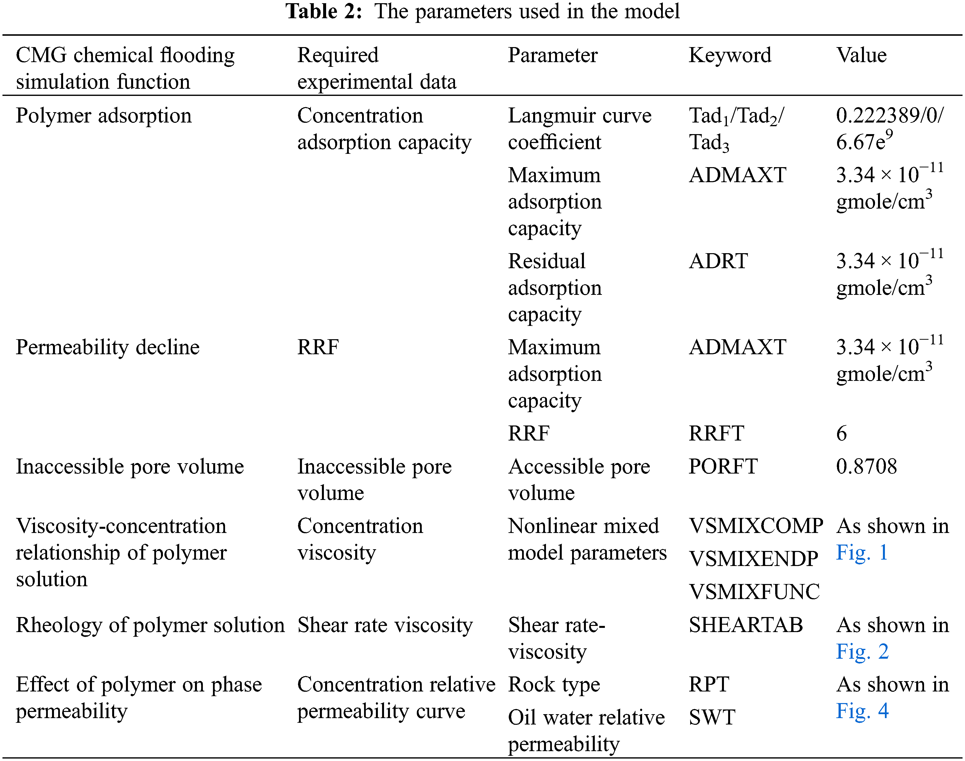
According to the test content, we selected the CMG simulator with a mature chemical flooding simulation for numerical simulation inversion and established a 10 × 1 × 1 one-dimensional grid model with a grid step of 1 cm × 2.5 cm × 2.5 cm. The initial temperature of the simulation was 40°C, the pressure was 101.3 kPa, the permeability was 94.657 mD, the porosity was 16.61%, and the injection rate was 0.2 mL/min. After saturating the core, we first performed water flooding. Then, we injected a polymer concentration of 0.15% and performed subsequent water flooding. The parameters used in the model are shown in Table 2.
4.2 Sensitivity Analysis of Polymer Parameters
The parameter sensitivity analysis of recovery and injection pressure is carried out based on the established model. In the process of recovery fitting, the more sensitive parameters are RRF and adsorption value. And in the process of injection pressure fitting, the more sensitive parameters are the viscosity of polymer solution, the maximum adsorption capacity of polymer, and RRF.
The viscosity parameters of polymer solution mainly affect the injection pressure. The greater the viscosity, the greater the injection pressure. The polymer adsorption value affects the final shape of the recovery curve, and the maximum polymer adsorption also affects the injection pressure. RRF affects the shape of the recovery curve to a certain extent and has a great influence on injection pressure.
The numerical simulation inversion needed to fit the degree of recovery, injection pressure, and water cut. The key to fit the experimental data was the adjustment of parameters. Because of the many model parameters and large adjustable degrees of freedom, to avoid the arbitrariness of parameter modification, the adjustable range of reservoir model parameters had to be determined when fitting. Doing so ensured that the model parameters could be modified within a reasonable and acceptable range.
1. Adjustment of porosity: according to the experimental results of characteristic parameters of polymer flooding, the core porosity was between 15% and 21%. During the fitting process, a small adjustment could be made within this range.
2. Adjustment of permeability: because the gas logging permeability of the measured core was 26.50–126.08 mD, there were large changes in plane and longitudinal direction. A large range of adjustment can be made to the permeability value within this range during the fitting process.
3. Adjustment of compressibility coefficient of rock and fluid: the variation range of these coefficients was generally small and could be treated as determined parameters. Because of the influence of indoor temperature, we made some necessary adjustments to the compressibility coefficient of rock and fluid in the process of fitting.
4. Adjustment of relative permeability curve: because of the heterogeneity of the core, the measured relative permeability curve reflected the situation of only a limited area. Thus, it could be treated as an uncertain parameter. We gave each section an appropriate initial value and adjusted it significantly according to the actual dynamic situation.
5. Adjustment of characteristic parameters: the adjustment of parameters, such as polymer adsorption, inaccessible pore volume, RRF, and polymer solution viscosity, directly affected the experimental results. We conducted a sensitivity analysis for these parameters to determine the influence degree of each parameter, which will be more targeted in fitting and adjustment.
By setting the polymer characteristic parameters obtained from the experiment in CMG software, we carried out the fitting of the recovery degree and injection pressure with different injection volumes. We obtained the final fitting results shown in Figs. 6 and 7. The fitting results were good, which further verified the reasonableness of the model and parameter setting and also provided a reference and basis for the history fitting, which holds great significance to guide the actual reservoir development.

Figure 6: Recovery degree fitting result
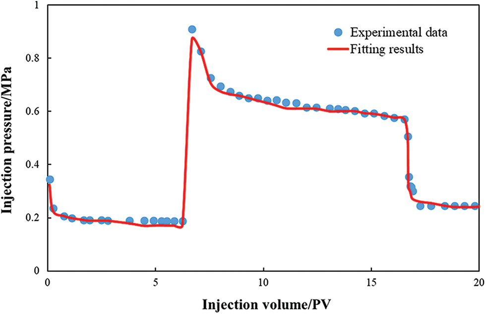
Figure 7: Injection pressure fitting result
Following are the conclusions of this study:
1. The CMG STARS simulator was suitable not only for large-scale reservoir simulation but also for small-scale indoor experiment simulation of polymer flooding. It well described the mechanism of polymer flooding, including polymer adsorption, permeability decline, inaccessible pore volume, viscosity-concentration relationship, rheology, and the effect of polymers on relative permeability. The experimental data required for the simulation could be obtained through indoor experiments, including concentration-adsorption, RRF, inaccessible pore volume, concentration-viscosity, shear rate-viscosity, and concentration-phase percolation curves.
2. It can be difficult to directly use the measurement results of physicochemical parameters in polymer flooding in numerical simulation. According to the conversion equation provided in this study, the experimental results of polymer characteristic parameters measured could be converted into the data needed in the numerical simulation, which realized the organic combination of physical and numerical simulations.
3. We identified some errors in the data obtained from the experimental measurement. Therefore, in the process of numerical simulation inversion, the parameters in the model also had to be adjusted. This required the analysis of each parameter, which had to be controlled within a reasonable and acceptable range, to improve the rationality and accuracy of the inversion. The indoor experiment fitting results could provide more reasonable parameters for the actual reservoir history fitting and then improved the rationality and degree of the actual reservoir history fitting, which holds great significance to the development of the actual reservoir.
Funding Statement: This paper was supported by Hubei Provincial Natural Science Foundation of China (Grant No. 2020CFB377) and the National Natural Science Foundation of China (Grant No. 52104020).
Conflicts of Interest: The authors declare that they have no conflicts of interest to report regarding the present study.
1. Lu, J. T. (2021). Application of numerical simulation technology in optimizing polymer flooding scheme of M reservoir. World Petroleum Industry, (2), 63–69. [Google Scholar]
2. Hu, S. (2021). Field application effect of TS1200 salt resistant polymer flooding in lamadian oilfield. Daqing Petroleum Geology and Development, (1), 117–121. DOI 10.19597/j.issn.1000-3754.202004016. [Google Scholar] [CrossRef]
3. Mahon, R., Oluyemi, G., Oyeneyin, B., Balogun, Y. (2021). Experimental investigation of the displacement flow mechanism and oil recovery in primary polymer flood operations. SN Applied Sciences, 3, 557. DOI 10.1007/s42452-021-04360-7. [Google Scholar] [CrossRef]
4. Wang, X. R. (2020). Mobility optimization design of polymer/surfactant binary compound flooding in offshore oilfield. Fault Block oil and Gas Field, (3), 344–349. [Google Scholar]
5. Li, Y. T., Kong, B. L. (2019). The technical way to improve the field application effect of ASP flooding. Journal of Southwest Petroleum University (Natural Science Edition), (4), 113–119. [Google Scholar]
6. Lu, X. G., Cao, B., Xie, K., Cao, W. J., Liu, Y. G. et al. (2021). Enhanced oil recovery mechanisms of polymer flooding in a heterogeneous oil reservoir. Petroleum Exploration and Development, (1), 169–178. DOI 10.1016/S1876-3804(21)60013-7. [Google Scholar] [CrossRef]
7. Zampieri, M. F., Ferreira, V. H. S., Quispe, C. C., Moreno, R. B. Z. L. (2020). History matching of experimental polymer flooding for enhanced viscous oil recovery. Journal of the Brazilian Society of Mechanical Sciences and Engineering, 42, 205. DOI 10.1007/s40430-020-02287-5. [Google Scholar] [CrossRef]
8. Liu, S., Xu, C., Su, W., Wei, Q., Liu, Y. (2021). Research progress of produced fluid treatment in offshore polymer flooding field. Oilfield Chemistry, (2), 374–380. DOI 10.19346/j.cnki.1000-4092.2021.02.030. [Google Scholar] [CrossRef]
9. Lamas, L. F., Botechia, V. E., Schiozer, D. J., Rocha, M. L., Delshad, M. (2021). Application of polymer flooding in the revitalization of a mature heavy oil field. Journal of Petroleum Science and Engineering, 204, 108695. DOI 10.1016/j.petrol.2021.108695. [Google Scholar] [CrossRef]
10. Suri, Y., Islam, S. Z., Stephen, K., Donald, C., Thompson, M. et al. (2020). Numerical fluid flow modelling inmultiple fractured porous reservoirs. Fluid Dynamics & Materials Processing, 16(2), 245–266. DOI 10.32604/fdmp.2020.06505. [Google Scholar] [CrossRef]
11. Hu, J., Li, A., Memon, A. (2020). Experimental investigation of polymer enhanced oil recovery under different injection modes. ACS Omega, 5(48), 31069–31075. DOI 10.1021/ACSOMEGA.0C04138. [Google Scholar] [CrossRef]
12. Zhang, J. L., He, S. M., Liu, T. J., Ni, T. L., Zhou, J. et al. (2021). Visualization of water plugging displacement with foam/gel flooding in internally heterogeneous reservoirs. Fluid Dynamics & Materials Processing, 17(5), 931–946. DOI 10.32604/fdmp.2021.015638. [Google Scholar] [CrossRef]
 | This work is licensed under a Creative Commons Attribution 4.0 International License, which permits unrestricted use, distribution, and reproduction in any medium, provided the original work is properly cited. |