Fluid Dynamics & Materials Processing

DOI: 10.32604/fdmp.2022.021860

ARTICLE

Numerical Analysis of a Microjet-Based Method for Active Flow Control in Convergent-Divergent Nozzles with a Sudden Expansion

Abdul Aabid1,*, Sher Afghan Khan2 and Muneer Baig1

1Department of Engineering Management, College of Engineering, Prince Sultan University, Riyadh, 11586, Saudi Arabia
2Department of Mechanical Engineering, Faculty of Engineering, International Islamic University Malaysia, Kuala Lumpur, 50728, Malaysia
*Corresponding Author: Abdul Aabid. Email: aaabid@psu.edu.sa
Received: 09 February 2022; Accepted: 18 April 2022

1  Introduction

Fluid flows undergoing abrupt axisymmetric expansions represent a complex problem in fluid-dynamics and can be found in a variety of fields and related technological applications. A circular tube is used with a smooth inner surface in most cases. Low pressure is created in the wake region due to a sudden increase in the duct area. The base pressure and flow-field is complex at the base region and is characterized by flow separation and reattachment. In some cases, the experiments were conducted with a sudden expansion duct and with ribs, cavities, and splitter plates. All these studies aimed to minimize base drag. Only a few studies showed that they had used dynamic control for the flow regulations. This study uses dynamic control in the form of jets of 1 mm diameter to regulate base pressure with a microjet at the base and duct; the ducts and wall combinations study are lacking in the literature. One study focuses on flow past cylinder by reference [1].

The ribs are passive control devices to operate the duct’s flow with sudden expansion [2]. Furthermore, the studies have also focused on control devices by changing the dimensions of annular ribs to see the effects on flow control. For missile configurations, the cavities have been employed in the base region of the missile to control the flow and obtain the pressure differences with the impact of base cavities via experimental work [3]. Al-Khalifah et al. used a similar data optimization method like response surface methodology [4] by using an effective supersonic nozzle with an abrupt increase in duct parameter to investigate wake pressure.

A numerical method was also critical to solving such problems after studying passive flow management through the investigational and numerical computing approaches. For fluid-flow analysis, the most common practice is the computational fluid dynamic (CFD) method. Undeniably, this technique was utilized by several researchers related to the current work. Both passive and active control methods have been used well for the CFD investigation over the last two decades. Turbulence modeling is a critical part of the fluent study; for compressible flows, a density-based model has been found in most cases. Via CFD investigation, it was proven that flow control via tiny jets is beneficial to regulate pressure in the separated region at large NPR when dynamic control as small jets from the nozzles flowing under favorable pressure in a CD nozzle [5,6]. Additionally, CFD was used to investigate external flow formation over different types of airfoils like CH10 [7], and wedge [8,9]. The flow control method in a bluff body was also found using non-circular in a front face [10,11] and splitter plate [12,13] with the CFD approach.

In fluid flow analysis, a nano-fluid in different temperature conditions was also analyzed using the CFD approach. In such studies, an expanding area was used to explore the 2-D magnetohydrodynamic steady boundary layer flow of a viscous liquid [13] and that shows an effective response based on the hybrid nano-fluids. For a similar study, thermal analysis of a hybrid-nanofluid solar collector and storage system [14] was considered a key point for the flow particles. The author conducted a numerical investigation on heat transmission via hybrid nano-fluid within a porous ring between a crisscrossed triangle and several cylinders beneath an angled magnetic arena using the COMSOL model [15]. It was a qualified study of nanoparticles based on water through nanoparticles over an exponentially quicker radiative Riga plate surface [16].

CFD can produce flow formation contours in all studies and determine the fluid properties. The CFD method is used to do the parametric study of the nozzle and shows the fluid flows inside the nozzle via contours and plots for each case. Furthermore, a streamlined formation can show the building of the flow inside the duct [17]. Apparat from CFD, a data optimization method, also became popular in a recent investigation. Several studies have been found regarding base pressure control with a microjet at the base in recent years using numerical simulations [18–25]. Similar to the present model, however, the location of microjet and those effects have not been reported to this author’s best knowledge. Hence, this study intends to explore the influence of microjet location on base flow control using the CFD method.

2  Computational Fluid Dynamics

The complete set of equations in terms of conservation of mass, momentum, and energy can be written for compressible ideal gas flow [26,27],

∂ρ∂t+∂∂xi(ρ¯u~i)=0 (1)

∂∂t(ρ¯u~i)+∂∂xj(ρ¯u~ju~i)=−∂p¯∂xi+∂∂xj(σ~ij−ρui′′uj′′¯) (2)

∂∂t(ρ¯E~)+∂∂xj[ρ¯u~j(E~+p¯)]=∂∂xj[u~i(σ~ij−ρui′′uj′′¯)]−∂∂xjq~j+∂∂xj[−cpρuj′′T′′¯+ui′′σij¯−ρuj′′12ui′′ui′′¯] (3)

where ρ¯,u~i,p¯ and E~ are the parameters demonstrating the density, turbulent velocity, pressure, and energy? The parameters with a bar reflect the time-averaged values.

The Navier-Stokes equations are transformed in a Reynolds Stress τ~ij with the average Reynolds technique. The equation is called Average Navier Stokes of Reynolds (RANS),

u~j∂∂xj(u~i)=−1ρ∂p¯i∂xj + ∂∂xj(μρ∂∂xju~i)+∂(τ~ij)∂xj (4)

With τ~ij=−ρui′′uj′′¯=−23ρ¯kδij+μtSij & Sij is strain rate,

Sij=(∂u~i∂xj + ∂u~j∂xi)−23∂u~k∂xkδij (5)

μt is eddy viscosity,

μt=cmρk2ε (6)

and cm=0.09 . Turbulent kinetic energy k=12ui′uj′¯ and the pliability not considered.

The standard k−ε turbulent model is the turbulence model employed to find the solution of the Reynolds Stress τ~ij . This model provides reasonably good results for internal flow. Launder and Spalding [27] introduced this turbulence model; typically, the model is used with a two k and ε transport equations. Turbulent model for normal k−ε written as,

∂(ρ¯k)∂t + ∂(ρ¯ku~j)∂xj=∂∂xj[μtρ¯k∂k∂xj]+2μtSijSij−ρ¯ε (7)

∂(ρ¯ε)∂t + ∂(ρ¯εu~j)∂xj=∂∂xj[μtρ¯ε∂ε∂xj]+c1εεk2μtSijSij−c1ερ¯ε2k (8)

Then Eqs. (7) and (8) are stated that σk=1.00 ; c1ε=1.44 ; c1ε=1.92 are constant variable for the model. The RHS of Eqs. (7) and (8), the parameters are transmission, production of k , and ε .

ANSYS FLUENT 18.0 is utilized to simulate how the fluid flows from the nozzle. The examination aims to determine pressure values in the wake and flow pattern in the duct and the impact of the microjet as a dynamic flow control management in three different cases. The microjet controller controls the base pressure of 13 mm, the same as the experimental investigation located at the PCD. Fig. 1 shows the model and design at the designed inertia levels.

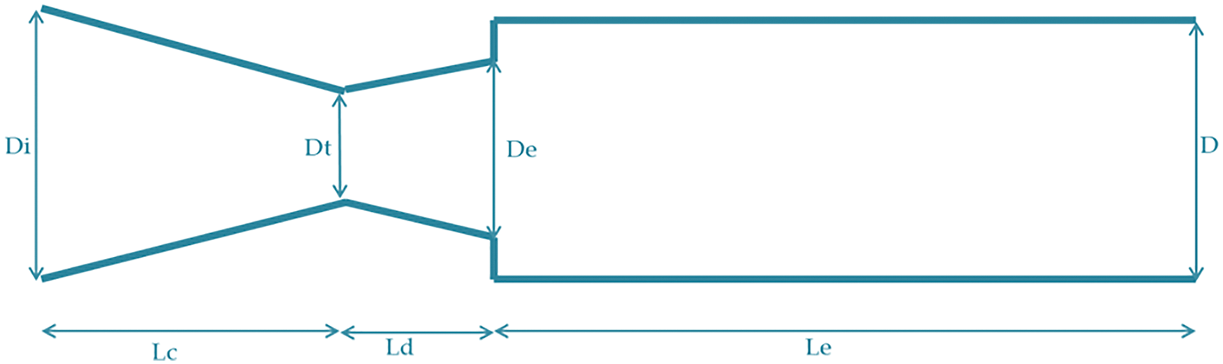
Figure 1: Geometrical model

A common approach was used to build the model, taking the fluid area’s points, lines, and surface into account. The simple geometrical dimensions and shapes were followed to design a nozzle in the 2D process. Points and lines are used, and the surface is then created from the sketch to the whole geometric shape. The nozzle has various parts; therefore, the split surface substitute is selected, and planes were divided into multiple regions to obtain a fine mesh on the large-density region. The faces, meanwhile, are distributed into numerous tiny faces to make a fine mesh at various nozzle positions.

In the nozzle, the boundaries were allocated by choosing each line of the segments. The flow is passing through the left to right. For inlet, three edges were selected with four different cases, which are:

1.    Without control-only left vertical edge (convergent inlet face)

2.    With control at base-two line left vertical edge and baseline split of 1 mm

3.    With control at wall-two lines left vertical edge and wall line split of 1 mm

4.    With control at both base and wall-three lines left vertical edge, baseline, and wall split of 1 mm

Next, the outlet right vertical edge, wall as all top edges, and symmetry as an axis line were selected. Fig. 2 indicates the boundaries assigned.

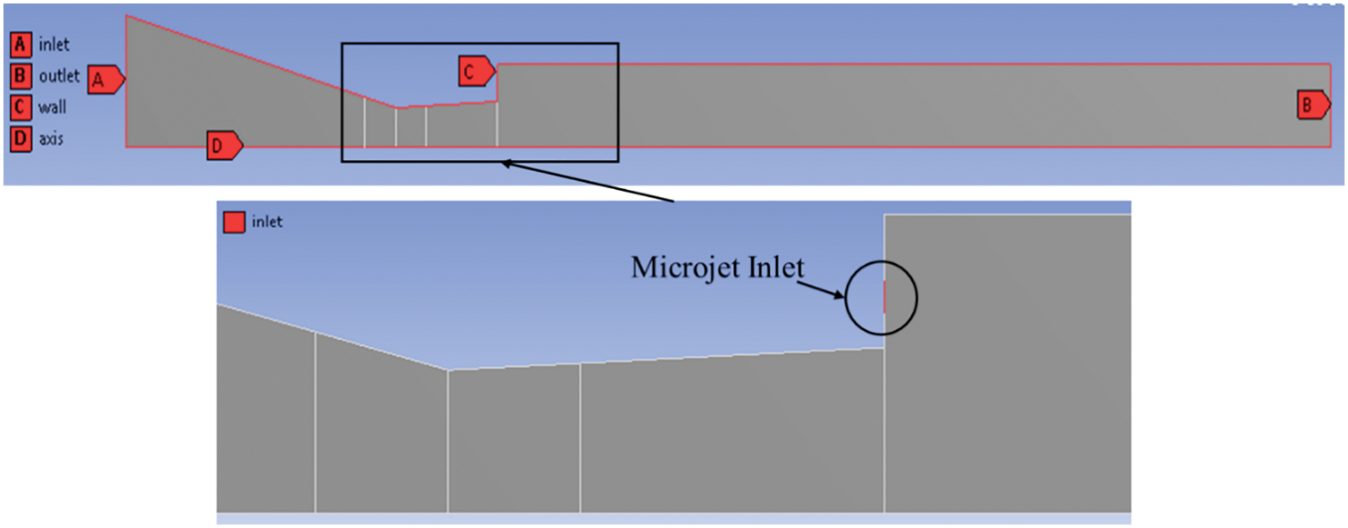
Figure 2: 2D nozzle with sudden expansion duct

In the CFD process, meshing is essential. The structured mesh is utilized for the 2D model by choosing the free face type of mesh type in the present case. The standardized mesh form was generated, and the element’s size was allocated.

The mesh metric statistics with skewness and element consistency have been rechecked, and the typical value is 7.057×10−2 and 0.66946, respectively. Similarly, the skewness and element consistency were rechecked when the microjets were used, and the mean value is 5.5031×10−2 and 0.6567, respectively. As per the ANSYS fluent guidance, the skewness and element quality values are within limits [28]. In the zoom view of Fig. 3, the high-dense mesh can be seen. Fig. 3 suggests the 2D model’s mesh for the non-microjet active control case; the number of elements is 154,288 (15,922). Standard wall functions were applied near-wall treatment. A wall y + < 5 was used as these were determined to be sufficiently accurate. The grids fulfilled the necessary y + conditions.

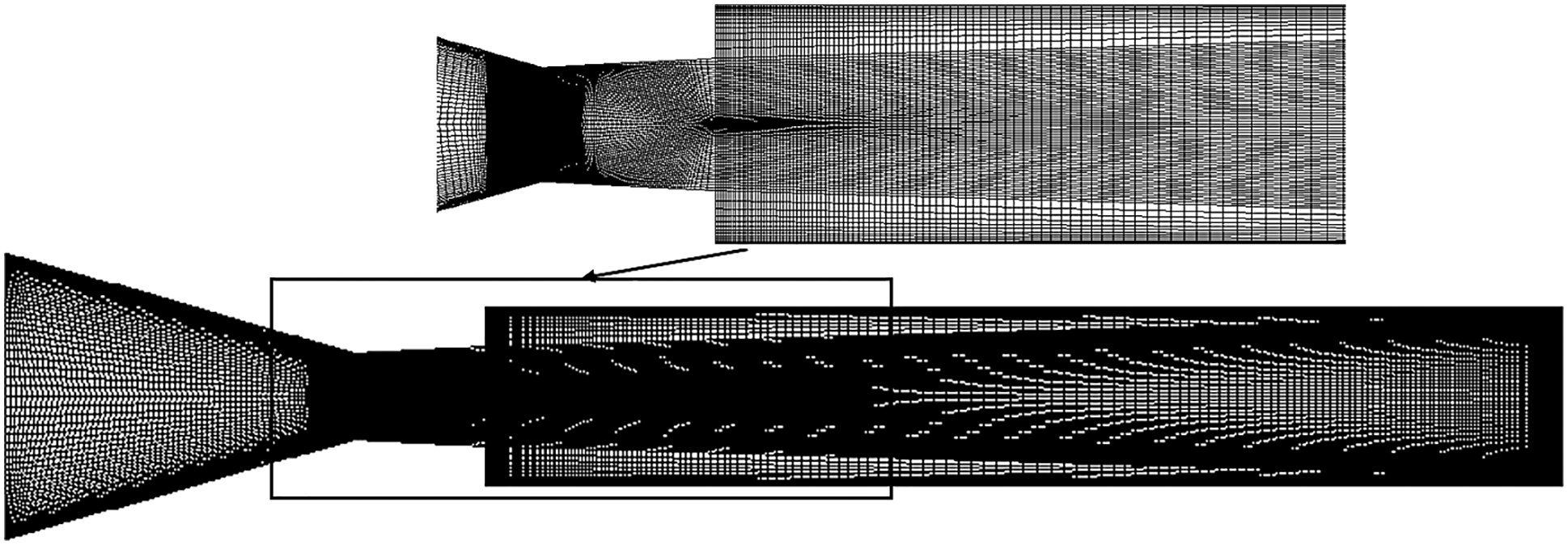
Figure 3: 2D mesh model without control

An implicit solver based on density is used for high-speed flows due to significant changes in density. The calculations of the fluid flow analysis for the nozzle were performed using RANS equations with a k−ε turbulent model [23], as per the earlier discussion of the equation that governs the flow and models which take care of the turbulence. The chosen flow medium is air, and Sutherland’s air behaves like the ideal gas and viscosity [29]. The boundary conditions applied are NPR for a Mach number and ambient pressure at the duct’s exit. The operating pressure was set to zero because the current issue is a form of compressible flow. Cell-face quantities are measured using a multi-dimensional linear reconstruction approach [30]. A Taylor series expansion of the cell-cantered solution around the cell centroid solution achieves better accuracy on the faces of the cells [31].

3  Results and Discussion

Based on the problem definition (Fig. 1) the different results have been made considering parameters of CD nozzle sudden expansion duct. In addition, the FVM has been validated with experimental results and mesh independence study was shown successfully.

3.1 Finite Volume Method Validation

3.1.1 Mesh Independence Study

Before we begin the simulations, mesh independence analysis is compulsory. The wall pressure was investigated for MIS for L/D = 10, Mach M = 1.87 at NPR = 3 for no control case. The different types of mesh mentioned are coarse, medium, & fine. The number of elements (nodes) that form the mesh form of the course is 7,996 (8,625), the number of elements for the medium is 12,321 (13,821), and the number of elements for the fine mesh is 16,312 (17,102). The computational time needed for the coarse, medium, & fine meshes to reach convergence was 892, 1130, & 1290 s. Unlike the coarse & medium mesh, the medium and fine mesh has a maximum error and minimum error of 3.56% & 2.28%, respectively. The wall pressure results of the fine mesh were similar to the experimental wall pressure results. The skewness and element consistency were rechecked after selecting the fine mesh to advance the simulation work further. Therefore, further experiments with a fine mesh of the CFD model have continued. The results were obtained using the Intel(R) Core (TM) i9-7980XE CPU operating at 2.60 GHz, 64.0 GB RAM, and Windows-10 64-bit OS (Fig. 4).

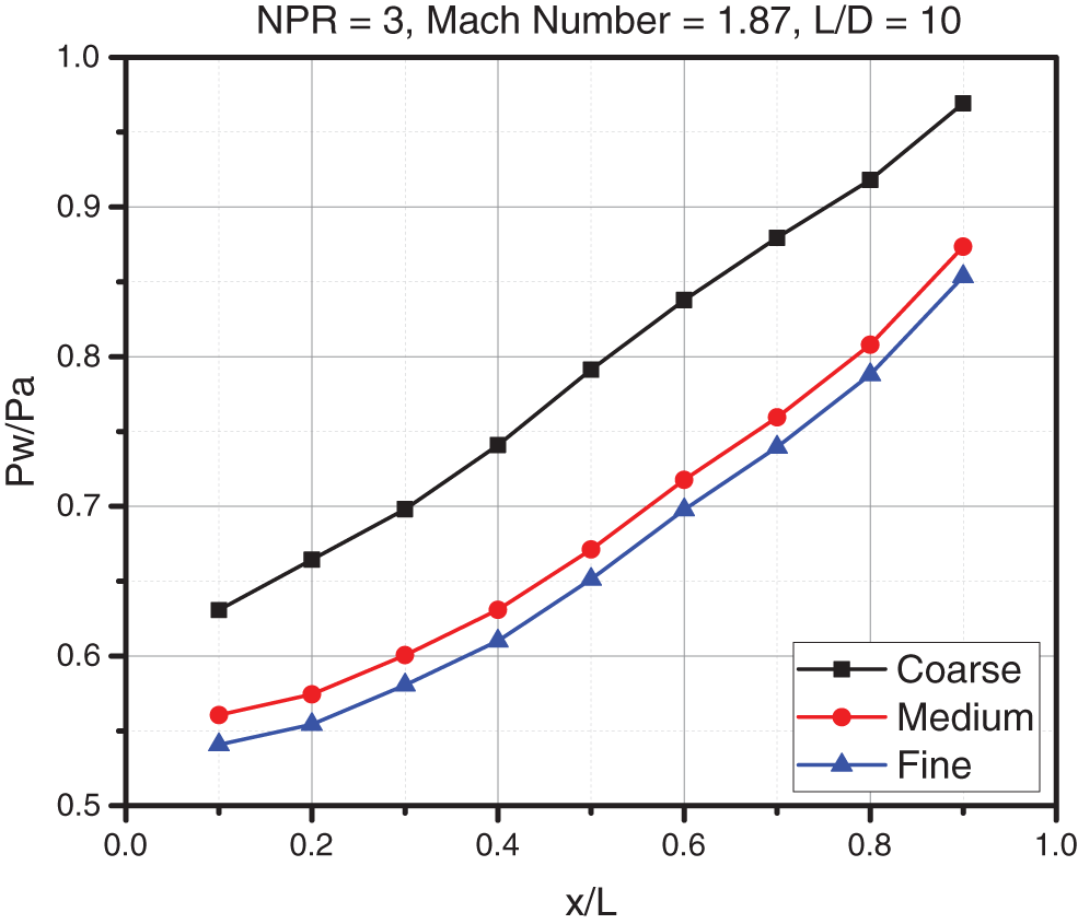
Figure 4: Mesh independence study

3.1.2 Validation with Existing Benchmark Study

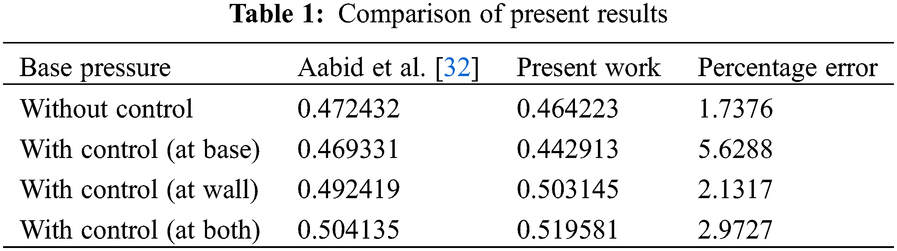
The experimental results obtained from the works of Aabid et al. [32] were considered to authenticate the outcomes acquired from the present finite volume model, as displayed in Table 1. The experimental data considered is Mach M = 2.58 for duct diameter ratio 1.8, NPR 5, and L = 10D. The findings agree with the wind tunnel test data. Table 1 illustrates the comparison of results.

3.2 Finite Volume Analysis

3.2.1 Pressure Contours

Figs. 5a and 5b show the pressure contour in the enlarged duct for different cases like without control, control at base, control at duct, and control at both the places for NPR = 3. Fig. 5a indicates a big recirculation zone at both corners. The corner pressure is low in the separated zone, and it is on the expected lines. The central jet carries high-pressure energy, which continues to be very high for a considerable distance. The low-pressure region ends before the main jet. Since simulation was done at NPR = 3, where jets face adverse pressure, for this case, Pe/Pa is 0.43. Whenever nozzles face adverse pressure, there will be an oblique shock wave at the exit of the nozzle resulting in considerable pressure, and the same is reflected in Fig. 5a.

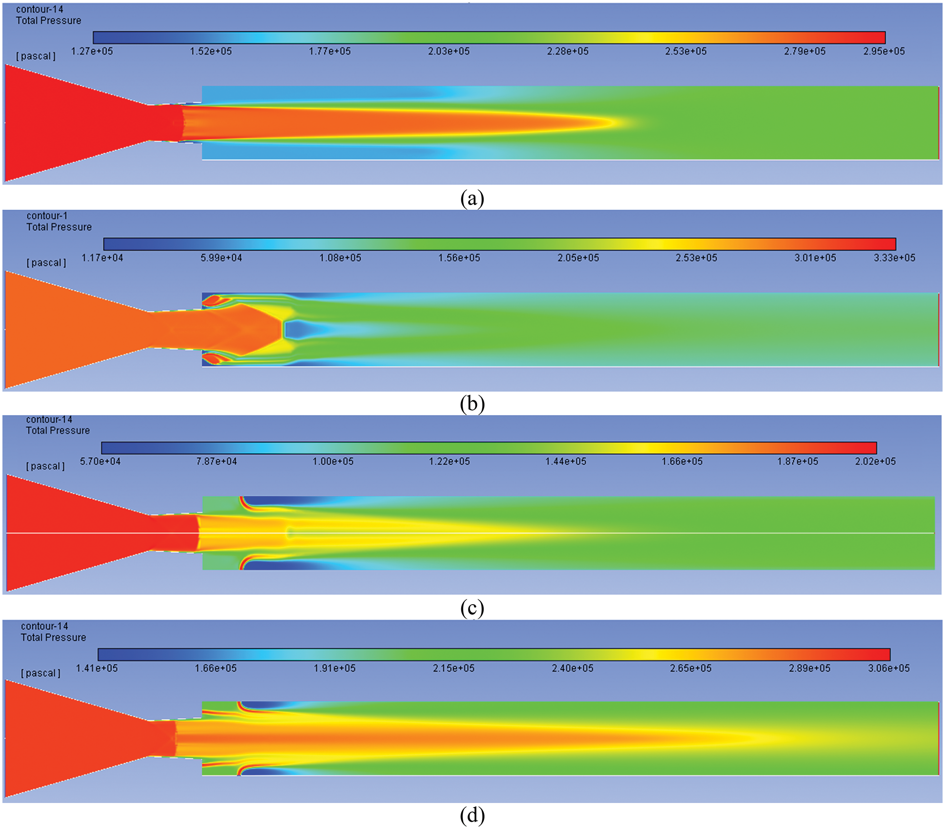
Figure 5: Pressure contours for NPR 3 (a) WoC (b) Control at base (c) Control at wall (d) Control at both

Fig. 5b displays the pressure field for the case when the control is located at the base. The low-pressure region seen without a control case is almost eliminated when control jets are located in the recirculation zone. The main jet is also modified due to the presence of the microjets; its length is reduced significantly. It is found that control jets at the base are most effective in decreasing the base suction. Fig. 5c shows the results of placing control jets in the duct. It is seen that the impact of the flow regulation is minimal in comparison to the case when control microjets were placed at the base; when control is at the base, it directly energizes the recirculation zone, resulting in higher pressure values. In this case, the pressure in the base corner has increased by 50% compared to the no control case. The influence of the main jet has propagated maintained considerable impact. Results of Fig. 5d are exhibited for the case when control is placed at both. The collective influence is appreciable since the kinetic energy is injected from the base and into the duct.

Figs. 6a–6d show the simulation results for NPR = 5. Owing to the rise in the NPR, the level of adverse pressure has gone down, and its value is 0.72. When we observe the results, without control case, the suction has reduced due to the increased NPR and reduced strength of the oblique shock waves. Because of an increase in the NPR values, there is a change in the shock wave strength, resulting in a modification in the flow structure inside the duct. It is seen that the microjets are effective as compared to the case when control was placed at the enlarged duct (Fig. 6c).

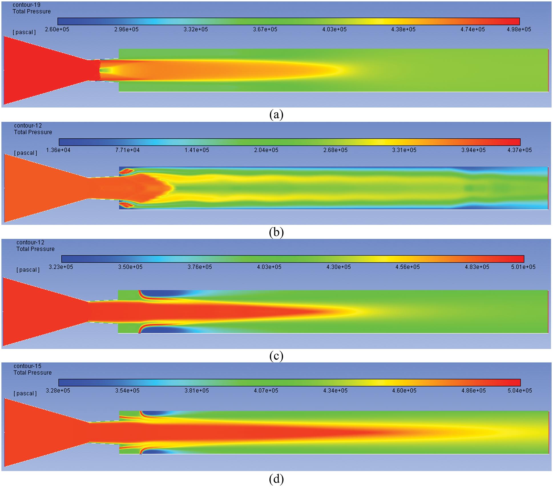
Figure 6: Pressure contours for NPR 5 (a) WoC (b) Control at base (c) Control at wall (d) Control at both

Similarly, when the control is placed at the base and the 1-D location of the enlarged duct simultaneously. The combined effect is the most compelling case. The pressure in the recirculation zone has increased considerably.

Figs. 7a–7d show the pressure contours at NPR = 7 with a level of expansion of 1.01. The jets are ideally expanded at this NPR, and the acoustic waves will accompany the flow. It seems to be very clean and free from shock waves. However, Mach waves are present across that the entropy remains constant. The base pressure is reasonably high compared to the lower Mach number, and the low-pressure region present at the base region is not visible (Fig. 7a). When the control is at the base, the recirculation zone of low pressure is seen; it may be due to the nozzle being operated at the design Mach number. The main jet, which used to have high-pressure energy, is not seen; instead, it is divided, and the central part has low pressure (Fig. 7b). When the active control is placed at the duct downstream of the flow, a low-pressure zone is formed due to the shielding effect (Fig. 7c). It is also seen that the active controls are placed at both places simultaneously, resulting in decreased base suction.

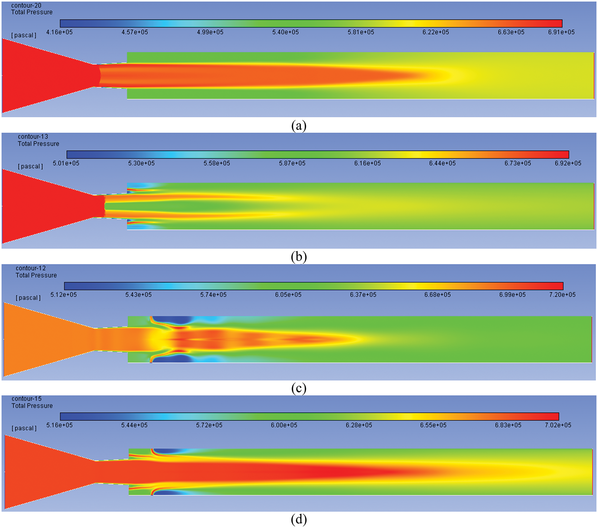
Figure 7: Pressure contours for NPR 7 (a) WoC (b) Control at base (c) Control at wall (d) Control at both

Figs. 8a–8d show pressure control results at NPR = 9 for under-expanded cases under the impact of a beneficial pressure. These results indicate a progressive decrease in the over-expansion level, and the base suction is getting reduced, increasing base pressure. The flow pattern for this case is on similar lines as discussed above.

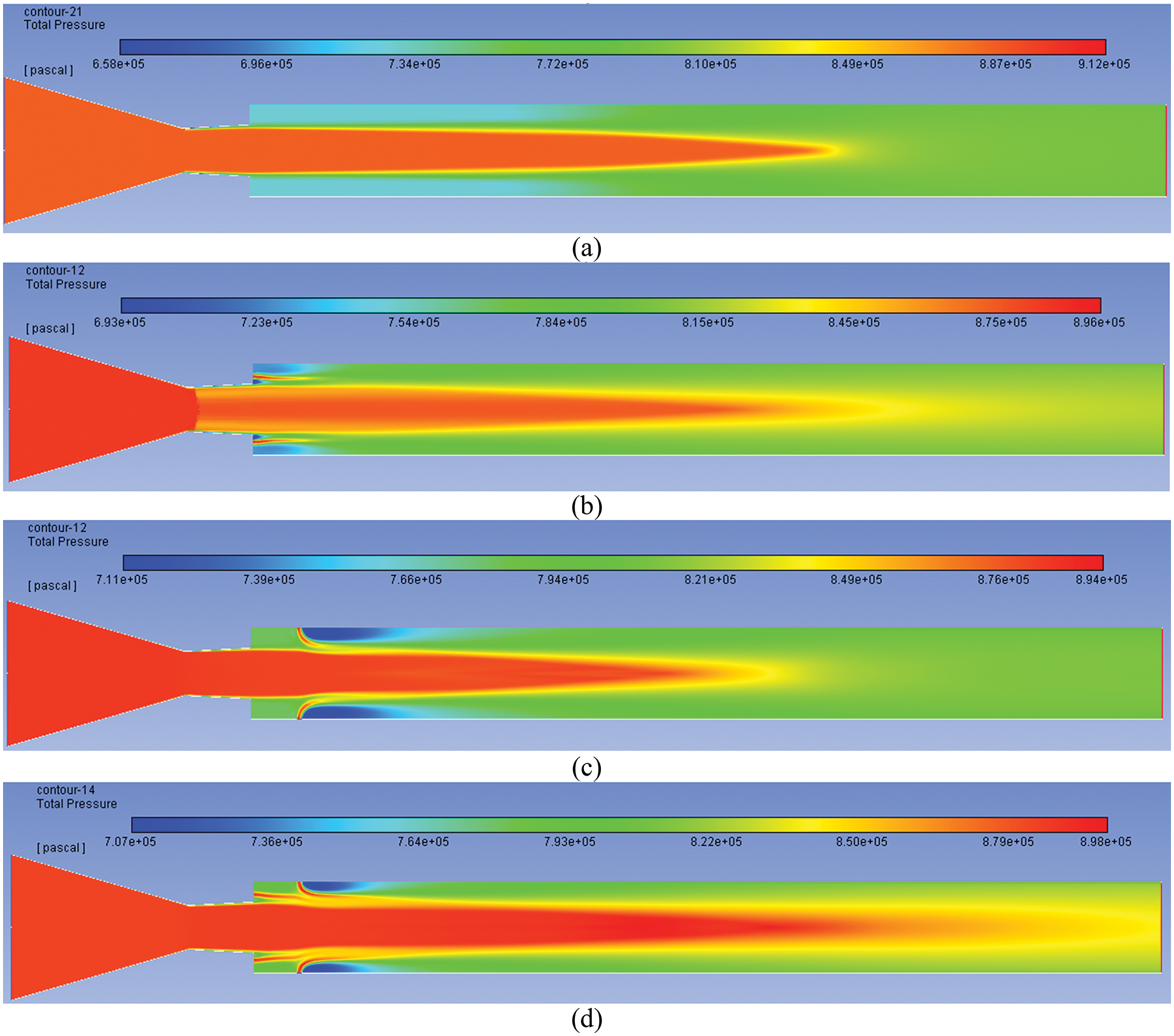
Figure 8: Pressure contours for NPR 9 (a) WoC (b) Control at base (c) Control at wall (d) Control at both

Figs. 9a–9d show results for NPR = 11 for under-expansion level of 1.6. There is a gradual enhancement in the pressure in the wake region with an increase in NPR even when control is not employed. When active controls are employed at the base, it creates a small low-pressure recirculation zone in the base corner; however, the pressure energy level is high in and around micro jets due to the injection of the air. Similarly, suction is created when the control is located in the duct despite air injection downstream around the injection location. When the control is placed at both the places in the corner, a substantial increase in the base pressure is attained. However, the downstream from the control jet at the wall has low-pressure spots as well.

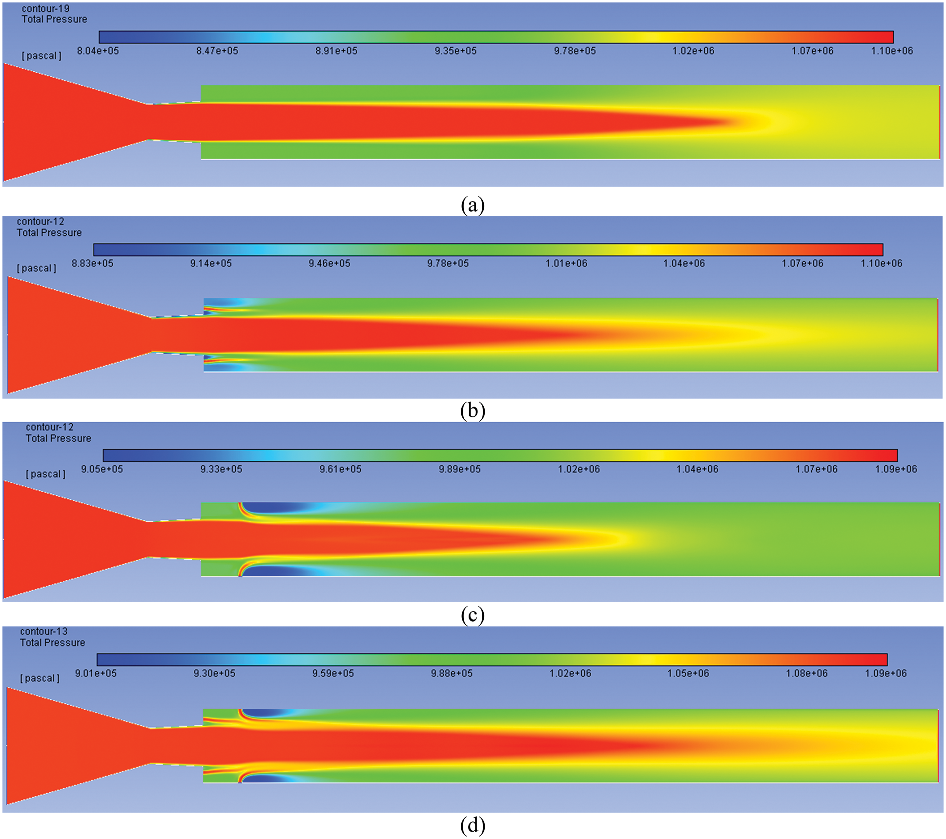
Figure 9: Contours for NPR 11 (a) WoC (b) Control at base (c) Control at wall (d) Control at both

Figs. 10a–10d show the Inlet-Outlet-Net Pressure of each NPR. Fig. 10a shows the results when control is absent. The inlet pressure is represented in black color, outlet pressure in red color, and net pressure is shown in blue color. The figure indicates a significant reduction in the outlet pressure due to the frictional effects. This loss is maximum at NPR = 3. However, there is a decrease in pressure loss with a rise in the NPR (Fig. 10a). When control was placed at the base as long as jets are over-expanded till NPR = 5, the pressure loss is considerable compared to the higher NPRs when jets are either correctly expanded or under-expanded, as seen in Fig. 10b. The significant pressure loss can be ascribed owing to the presence of a powerful oblique shock wave whose strength will decline with an increase in NPR owing to the decrement in the adverse pressure level. When the active flow regulation is placed at the duct at 1D, the significant pressure loss at lower NPRs 3 and 5 has declined, as the recirculation zone is energized due to the blowing at sonic Mach number (Fig. 10c). When control is placed at the base and the duct due to the blowing from the base and in the duct, there is a negligible difference in pressure as they are counterproductive due to their positioning.

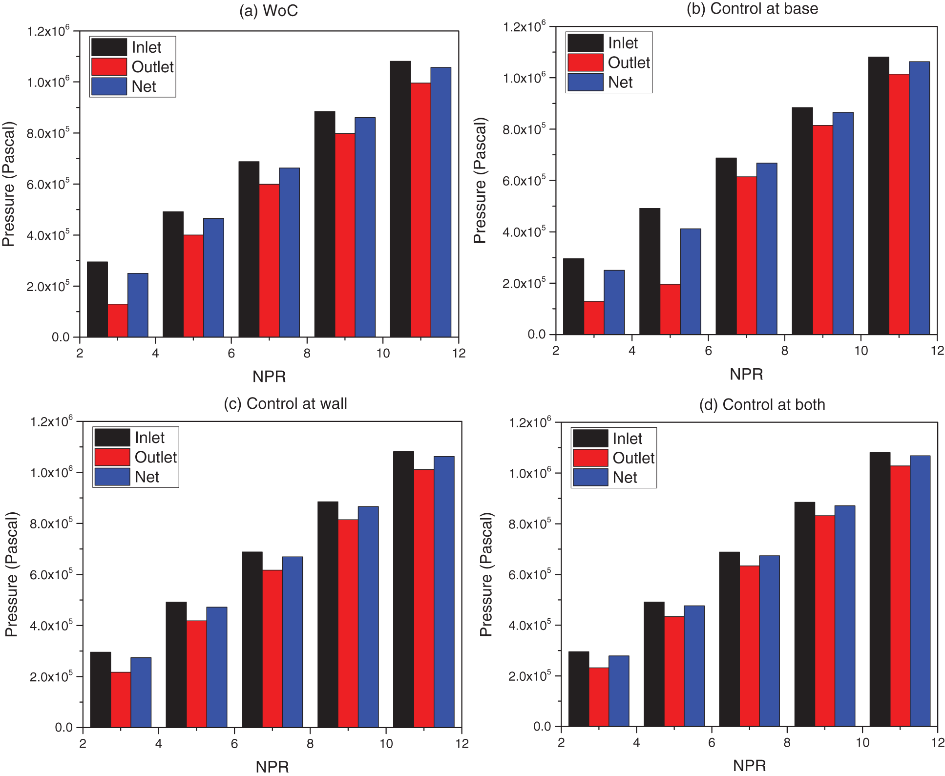
Figure 10: Inlet-Outlet-Net pressure of each NPR

Figs. 11a–11b show a comparison among inlet pressure, outlet pressure, and net pressure at NPRs in the array from 3 to 11. Fig. 11a shows a comparison in the outlet pressure regarding inlet pressure for various conditions like no control, flow regulator at the base, duct, as well as and the combined effects. At NPR = 3, the outlet pressure assumes identical values for no control and when control is located at the base. Later, when control is placed at the duct at both places, there is considerable growth in the outlet pressure. However, when the control is set at both locations, there is a negligible increase in the outlet pressure. It may be due to the flow’s excessive interaction, which in turn can leading to more losses. When we look at the results for NPR = 5, a marginal reduction in the outlet pressure is seen for the without control case. Once the tiny jet is employed at the base, there is more than a fifty percent loss of the outlet pressure. When dynamic control is used at both places, the combined effect is negligible compared to the control located at the base. This outlet pressure trend may be attributed to intense oblique shock waves at NPRs 3 and 5. When we observe the outlet pressure values for NPR = 7, 9, and 11, it is found that the outlet pressure for without control, control at base, at the duct, and combined effects do not show negligible variations in the outlet pressure. When NPR = 7, the nozzle is nearly correctly expanded, and at NPR = 9 & 11, it has under- expansion levels of 1.3 and 1.6. In all these cases at the nozzle exit, either Mach waves are present, or the expansion waves are not very strong compared to the shock waves; hence, this can be the cause for the slight change of outlet pressure.

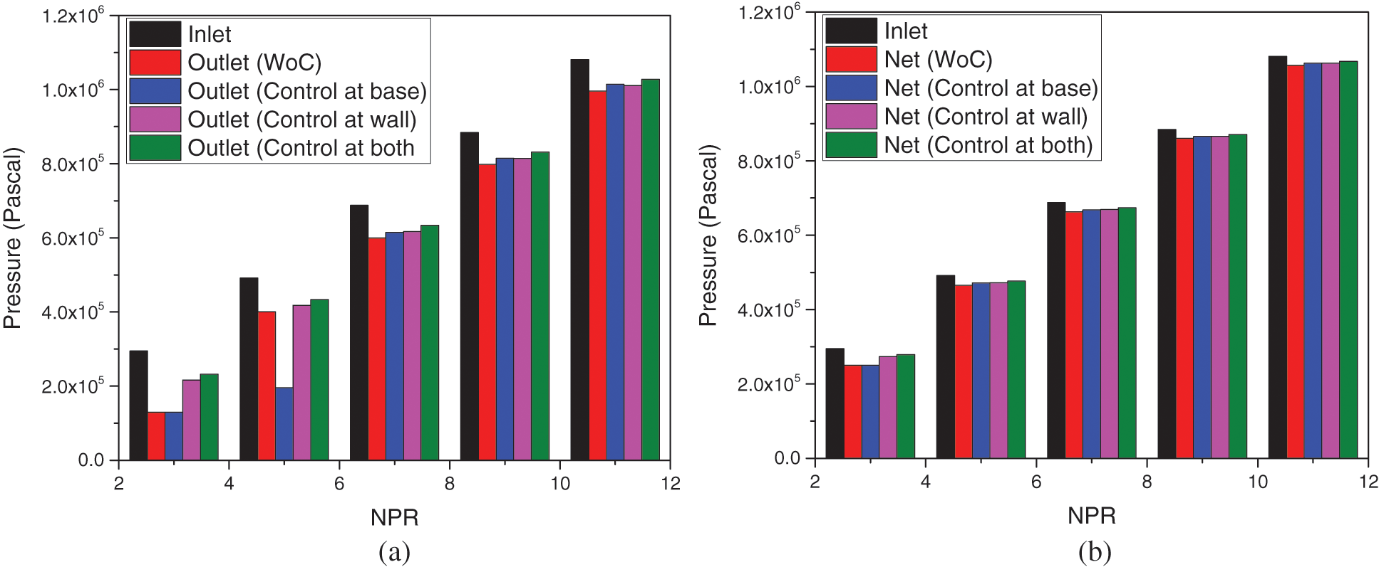
Figure 11: Comparison of (a) Outlet and (b) Net pressure

Fig. 11b displays net pressure as a function of NPR for NPRs in the range from 3 to 11. The figure shows that the net pressure is the same for all the cases irrespective of the control mechanisms with and without control and location. However, inlet pressure is more for all of the cases. This figure reiterates the conservation of energy.

3.2.2 Mach Number Contours

Mach number contours are shown in Figs. 12a–12d when NPR = 3. Fig. 12a shows Mach contour for NPR = 3 in the absence of the control mechanism. Due to a strong shock wave, the flow has decelerated to a large extent. When control is employed in the wake region around 1D, the flow Mach has increased, as shown in Fig. 12b. Fig. 12c shows the Mach contour when the active control is employed at the duct, increasing Mach number. The base corner Mach numbers remain low. When the control is used at the base and duct, even though the flow Mach number in the recirculation is low, yet in downstream, there is a considerable increase in the Mach number downstream to the duct due to the combined effect of the flow control mechanism.

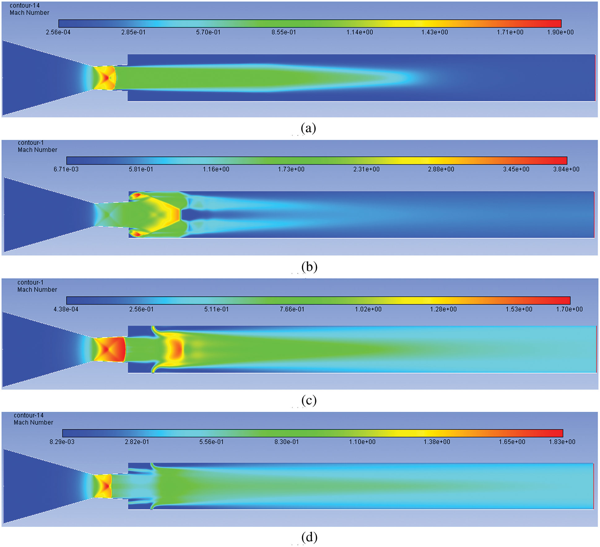
Figure 12: Mach number contours for NPR 3 (a) WoC (b) Control at base (c) Control at wall (d) Control at both

Results for NPR = 5 are presented in Figs. 13a–13d. Fig. 13a shows that the Mach number is meager with a rise in the NPR and a reduction in over-expansion. When control is placed at the base, the suction in the recirculation zone is reduced considerably compared to when NPR = 3, and even for NPR = 3 when control is at the base (Fig. 13b). For when the control mechanism is positioned at the tube, the impact on the flow is marginal, as witnessed in Fig. 13c. Finally, when flow control management is placed at both places it results in considerable change in the flow of the duct as the flow is energized due to the existence of the active control mechanism (Fig. 13d).

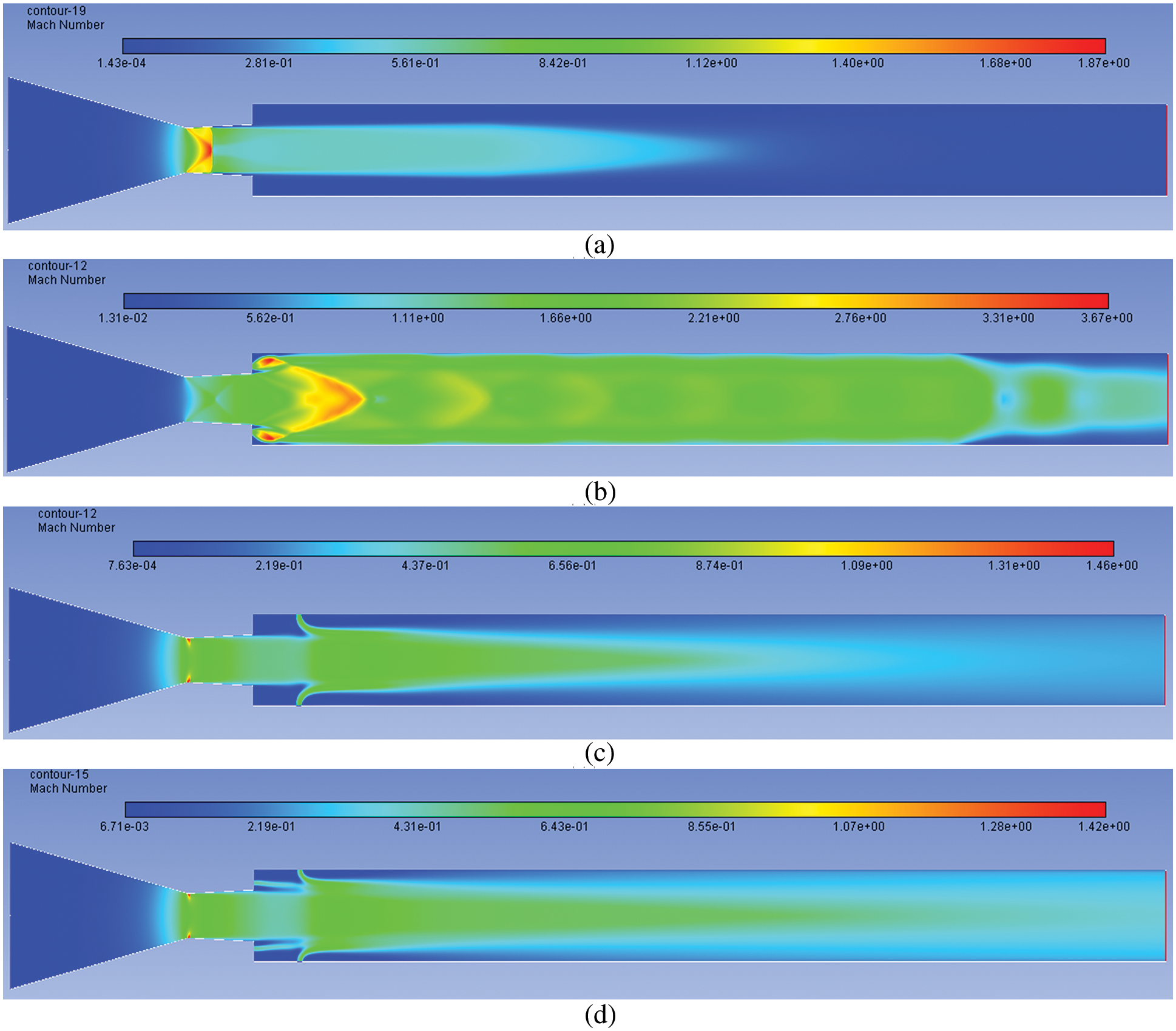
Figure 13: Mach number contours for NPR 5 (a) WoC (b) Control at base (c) Control at wall (d) Control at both

With a further increase in NPR, the Mach contour findings are represented in Figs. 14a–14d. This operating NPR = 7 is almost equal to the NPR needed for ideal expansion. Since Pe/Pa = 1.01, which is 1% more than the NPR required for proper expansion. At this NPR, the flow while exiting will be accompanied by the weak waves across them; there is no change in the entropy. Once we observe the stream without control, the flow pattern for a considerable distance around the wall is at a low Mach number (Fig. 14a). But when the control is placed at the base, it further slows down the flow field, as noticed in Fig. 14b. This implies that the presence of the Mach waves when control is initiated is counterproductive and affects further deceleration in the flow field of the tube. While the microjet is located in the duct, in this case, it is a single jet. It is normal to the flow direction, and has more effective results than the case when flow regulators are microjets, and where four jets are placed in the direction of the flow and not very effective (Fig. 14c). The combined effect is most effective when the control is placed at both.

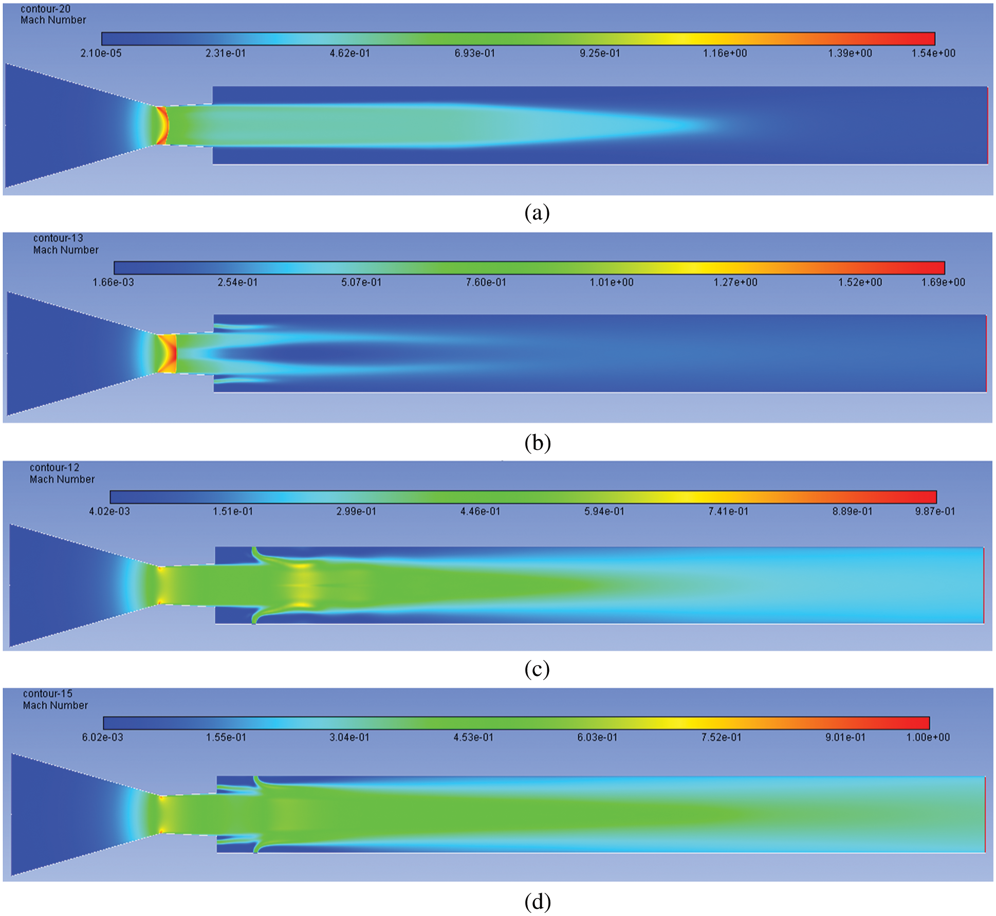
Figure 14: Mach number contours for NPR 7 (a) WoC (b) Control at base (c) Control at wall (d) Control at both

Figs. 15a–15d show the Mach contour results for NPR = 9. At this NPR, the level of expansion is 1.3. That indicates a 30% increase in the NPR level concerning design NPR. There is no appreciable change in the flow field with no control case (Fig. 15a). A marginal flow pattern changes when the control jets are placed at the base as this sonic jet’s injection is in the main jet flow direction (Fig. 15b). As we have earlier observed, when the control jet is located at a 1D position at the duct, it can influence the flow field to a great extent as the control is normal to the main jet (Fig. 15c). At last, the collective influence is most effective when control is located base and enlarged, as seen in Fig. 15d.

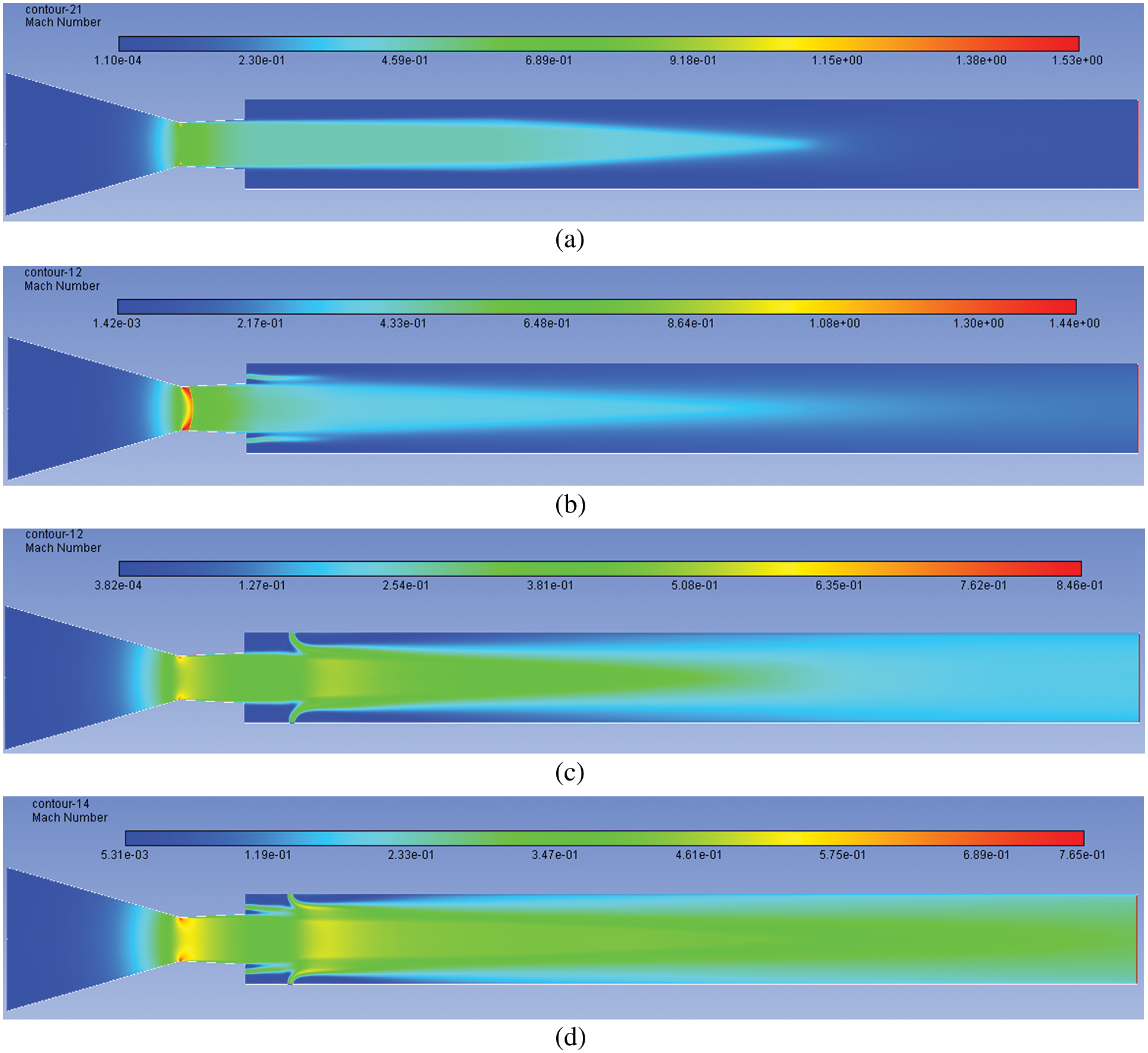
Figure 15: Mach number contours for NPR 9 (a) WoC (b) Control at base (c) Control at wall (d) Control at both

Mach contour results for the highest NPR = 11 tested are displayed in Figs. 16a–16d. At this NPR Pe/Pa = 1.6, the most advantageous level of under-expansion was observed, causing a maximum increase in the base and wall pressure. For without a control case, there is a considerable rise in the Mach number and the velocity of the stream field. This change is attributed to the increased level of under-expansion, resulting in a larger reattachment length and the expansion of the flow after exiting from the nozzle (Fig. 16a). Fig. 16b indicates that while the control is located at the base, there is a marginal increase in the Mach number of the flow field, as discussed earlier. For tiny jets, they are being placed at a 1D location in the tube resulting in a substantial increase in the flow the Mach number. The reasons are the same as when the control is placed at the base and the duct.

Figure 16: Mach number contours for NPR 11 (a) WoC (b) Control at base (c) Control at wall (d) Control at both

Figs. 17a–17d show the Mach numbers at the inlet, outlet, as well as the net Mach number. In the absence of control in Fig. 17a, it is seen that for all expansion levels in the current study, the inertia level is high at the outlet, and the net Mach number is relatively low compared to its exit, which is on the expected lines. In any case, net Mach is larger than Mach at the inlet. Fig. 17b shows the Mach numbers when control is placed at the base. The outlet Mach at NPR = 3 is unexpectedly more significant than other NPRs. At NPR = 3, the outlet Mach number is 0.6, and at all other NPRs, it is in the range of 0.4 to 0.3, and the trend of Mach numbers remains as seen without the control case. This topic needs more investigation to arrive at any proper conclusions. When the microjet is located at the duct, the Mach number achieved at the outlet is relatively low compared to when the control is located at the base. With the increase, the NPR downward trend is continuing as is seen in the previous case (Fig. 17c). When the control is placed at both the locations (i.e., at the base and the duct), it increases the outlet Mach numbers at NPR = 3, but still, its value is lower than what we got when the control was at the base. Only the outlet Mach number at NPR = 3 has shown typical behavior; otherwise, the Mach values at the inlet and the net Mach numbers follow the trend as expected.

Figure 17: Inlet-Outlet-Net Mach number of each NPR

3.2.3 Flow Formation in an CD Nozzle

Figs. 18a–18d show the Mach number vectors at NPR = 9 when the flow accelerating devices are operating under the effect of pressure more than that which is required by the design value. Fig. 18a indicates the development of the recirculation region when control is absent. Once the flow has come out from the nozzle, the flow attains larger Mach values. Fig. 18b shows the Mach number vector contour when control is located at the base. Due to the injection of energy through the control jets, the dead circulation zone is removed and there is an overall increase in Mach value across the entire flow field. When control is activated at the duct alone, the dead zone at the base corner almost remains intact; however, in and around the control jet flow field remains energized. Still, near the duct wall, the low-velocity region persists, and control cannot influence the flow field. That may be due to the location of the control, which is at a distance of 1D from the base.

Figure 18: Mach number 1.87 vector contours for NPR 9 (a)WoC (b) Control at base (c) Control at wall (d) Control at both

4  Conclusions

Built on the above debate, we have drawn the subsequent conclusions:

•   The control turns out to be very efficient once nozzles are being operated, either at design NPR or NPRs larger than design NPR. For lower NPRs, the pressure at the base is minimum; however, there is a gradual rise in the base pressure with the NPR. The air injection at the bottom is more effective than the one located at the duct section.

•   When the control is placed at the base, the 1-D location of the duct and the base simultaneously causes a maximum rise in the base pressure. The combined effect is the most effective combination. The pressure in the recirculation zone has increased considerably.

•   When the net pressure is considered for various NPRs in the range from 3 to 11, its value is the same for all the cases irrespective of the control mechanisms with and without control and their location. However, inlet pressure is more for all the cases. These results reiterate the conservation of energy.

•   When we look at the Mach contour, it is found that the flow field assumes lower velocity when the jets are over-expanded. However, with the progressive increase in the NPR, the flow field is getting energized. For nozzles with either correct expansion or under expansion, the Mach number is relatively high due to the growth of the jets and the increased reattachment length.

•   While the control is placed at both, the combined effect results in higher Mach numbers. The outlet Mach number at NPR = 3 is maximum irrespective of the control location. The variations in the control location have attained lower values at the duct and even for the case when microjets are placed at both locations.

•   When we look at the Mach numbers vector contour for without a control case, a dead zone is formed, but when it is employed at the base, this recirculation is eliminated by the control mechanism.

•   When we place control only at the duct, the dead zone persists. The dead zone is still there even though control is placed at the base and in a tube when the collective effect is viewed.

•   The flow control management in the tube adversely impacts the duct flow field.

•   The established computational fluid dynamics models can be utilized efficiently to predict the pressure at the base and walls under numerous running circumstances and eliminate the need for massive experimental work. This study is vital to aerodynamic engineers while choosing the most critical parameters to attain the necessary recirculation that impacts the base drag through an abruptly expanded flow process.

Acknowledgement: This research is supported by the Structures and Materials (S&M) Research Lab of Prince Sultan University. Furthermore, the authors acknowledge the support of Prince Sultan University for paying the article processing charges (APC) of this publication.

Funding Statement: The authors received no specific funding for this study.

Conflicts of Interest: The authors declare that they have no conflicts of interest to report regarding the present study.

This work is licensed under a Creative Commons Attribution 4.0 International License, which permits unrestricted use, distribution, and reproduction in any medium, provided the original work is properly cited.