Fluid Dynamics & Materials Processing

DOI: 10.32604/fdmp.2022.020020

ARTICLE

Simulation of Oil-Water Flow in a Shale Reservoir Using a Radial Basis Function

Zenglin Wang1, Liaoyuan Zhang1, Anhai Zhong2, Ran Ding2 and Mingjing Lu2,3,*

1Shengli Oilfield, Sinopec, Dongying, 257001, China
2Petroleum Engineering Technology Research Institute of Shengli Oilfield, Sinopec, Dongying, 257067, China
3Postdoctoral Scientific Research Working Station of Shengli Oilfield, Sinopec, Dongying, 257067, China
*Corresponding Author: Mingjing Lu. Email: mingjinglu2021@163.com
Received: 29 October 2021; Accepted: 21 December 2021

Nomenclature

1  Introduction

Water-driven development has been the most efficient and successful method of reservoir recovery for nearly a century. Currently, most of the oil reservoirs on earth are produced by water injection. According to incomplete statistics, there are more than 600 water-injected fields with more than 110,000 water-injected wells worldwide [1]. Therefore, any progress in modeling and predicting water-driven production increases is critical [2–7].

Water injection development is commonly employed in reservoir development because it maintains formation pressure and enhances oil and gas recovery. The coexistence of oil and water in water-driven reservoirs can be classified as an interface problem [5]. Submerged boundary method, finite element method (FEM), finite volume method and traditional finite difference method are commonly used to deal with such problems. The above methods make it challenging to interpret the information inside and outside the interface, especially about the irregular regions [8,9]. It is simple to ignore the existence of the interface and it is time consuming to generate a large number of meshes. Pre-processing and post-processing are inconvenient and require a large amount of mathematics. The main advantage of meshless techniques is that they do not require the division of a mesh; instead, they rely on the random selection of discrete nodes in the computational region, avoiding the challenges associated with mesh division. Therefore, we propose in this paper a meshless radial basis function method for numerical simulation of oil-water flow.

The radial basis function, also known as the distance basis function, is constructed using a one-dimensional distance variable. It benefits from a basic form that is independent of spatial dimensionality and isotropy. In the last few decades, radial basis function methods have attracted the interest of a large number of scholars in science and engineering [10–12]. Hardy [13] pioneered the use of radial basis functions and multisquare functions for topographic surface interpolation and irregular surface interpolation. Subsequently, Duchon et al. [14] developed thin-plate spline functions and compared and investigated 29 discrete data interpolation methods to solve common function interpolation difficulties. By examining the numerical results, he found that the MQ function proposed by Hardy and the TPS function proposed by Duchon had the highest numerical accuracy. These two types of functions are also the most commonly used radial basis functions in subsequent studies. Zhang et al. [15] have conducted extensive research on meshless methods based on the radial basis function collocation method. For partial differential equations with Neumann boundary conditions, a Hermite type of collocation method was proposed. Numerical investigations showed that the Hermite type of the collocation method greatly enhanced the numerical accuracy. Shivanian [16] proposed a partial radial basis point interpolation method for the two-dimensional time-component convection-diffusion-reaction equation in a gridless mode in the same year, and studied and proved the stability and convergence of the gridless method. In 2020, Oru [17] solved the two-dimensional elastic wave equation using a partial radial basis function method, and analyzed the stability of the method. and analyzed the stability of the method [18].

In this paper, the radial-based meshless method is used to solve the oil-water two-phase flow model in the reservoir. A one-dimensional example is used to demonstrate the accuracy of the method. Then, we compare the two-dimensional reservoir model with the finite difference method. Finally, the robustness of the method is evaluated in terms of Gaussian function parameters, time step and space step.

2  Mathematical Model

2.1 Basic Model

The model assumes (1) the external boundary of the reservoir is closed; (2) fluids and rocks are slightly compressible; (3) isothermal flow events, neglecting heat loss; and (4) oil and water are in two phases, and the two phases are not mutually soluble.

The oil-water two-phase flow equations in the reservoir are

∇[kkroμo∇po]+qosc=∂[ϕSo]∂t (1)

∇[kkrwμw∇pw]+qwsc=∂[ϕSw]∂t (2)

2.2 Radial Basis Function

Many researchers have conducted in-depth research on radial basis function (RBF), and have successfully applied radial basis function to different numerical methods, especially the meshless method.

Radial basis function refers to the function of r which only depends on radial coordinates ϕ(r)=ϕ(∥x−xj∥) , r=∥x−xj∥ where is the Euclidean distance between nodes x and xj. For any function, the radial basis function u(x) can be approximated as

u(x)=∑i=1nRi(x)ai+∑j=1mpj(x)bj=RT(x)a+pT(x)b (3)

where Ri(x) is the radial basis function, n is a number of radial basis functions, m is the number of polynomial basis functions. In order to determine the sum in Eq. (10), n field nodes contained in the support domain at calculation point x can be brought into Eq. (10).

Us=R0a+Pmb (4)

where Us={u1u2u3⋯um}T is the value vector of the node function, and the moment matrix of the radial basis function is

R0=[R1(r1)R2(r1)⋯Rn(r1)R1(r2)R2(r2)⋯Rn(r2)⋮⋮⋱⋮R1(rn)R2(rn)⋯Rn(rn)] (5)

The moment matrix of the polynomial is

PmT=[11⋯1x1x2⋯xny1y2⋯yn⋮pm(x1)⋮pm(x2)⋱⋯⋮pm(xn)] (6)

The coefficient vector of the radial basis function is

a={a1a2a3⋯an}T (7)

The polynomial coefficient vector is

b={b1b2b3⋯bn}T (8)

In Eq. (3), rk is defined as

rk=(xk−xi)2+(yk−yi)2 (9)

However, there are n + m variables in Eq. (5), and m constraints need to be added to solve the coefficient matrices a and b,

∑i=1npj(xi)ai=PmTa=0,j=1,2,⋯,m (10)

The following matrix equation can be obtained by simultaneous Eqs. (5) and (10):

U~s=[Us0]=[R0PmPmT0][ab]=Ga0 (11)

where

a0T={a1a2⋯anb1b2⋯bm} (12)

U~s={u1u2⋯un00⋯0} (13)

Because the matrix R0 is symmetric, the matrix G will also be symmetric. Then the coefficient vector can be solved

u(x)={RT(x)pT(x)}G−1U~s=ΦT(x)U~s (14)

where Φ(x) is the shape function vector,

ΦT(x)={RT(x)pT(x)}G−1={ϕ1(x)ϕ2(x)⋯ϕn(x)} (15)

The approximate solution uh(x) can be obtained.

The pressure equation is obtained by adding Eq. (1) to Eq. (2).

∇[(kkroμo+kkrwμw)n∇pon+1]=ϕCf∂P∂t (16)

and approximates the pressure equation P by a radial basis function,

P(x,y,z,t)=P(x,t)≈∑i=1Nainϕj(x) (17)

Substituting (17) into (16) and differencing the times gives

∇{(kkroμo+kkrwμw)n∇[ajn+1ϕj(x)]}=ϕCf[ajn+1ϕj(x)−ajnϕj(x)]∂t (18)

For all points in the solution domain, a linear system of equations is established according to Eq. (18), and a1n+1 , a2n+1 , ⋯ aNn+1 is solved layer by layer into Eq. (17) to obtain an approximate solution for the pressure P(x,y,z,t) . Then, the pressure is substituted into Eq. (2) to find the water saturation Sw at the next moment, and the oil-water two-phase flow simulation of shale reservoirs can be realized by solving in turn.

3  Numerical Examples

Based on the above radial basis function, oil-water two-phase flow theory. The following one-dimensional reservoir model is constructed, the reservoir permeability field is shown in Fig. 1. The size of the model is 400 m * 10 m * 10 m. The injection well IN1 is located on the left side of the model and the production well is located on the right side of the model. The injection rate is 10 m3/day, The Production rate is 10 m3/day and the production time is 1000 days. The time step is Δt=10 day and the space step is Δx=10 m. Gaussian radial basis function Rj(x)=exp⁡(−cd2)(c>0) is selected, and the parameter c is 200. Some physical property information is shown in Table 1. Eclipse is used to verify the accuracy of the method in this paper.

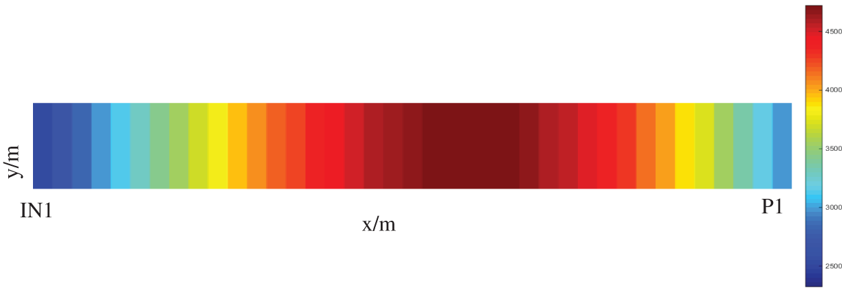
Figure 1: Permeability field

It can be seen from the daily oil production rate and the water saturation curve at 1000 days, as shown in Figs. 2 and 3. The accuracy of this method is basically consistent with that of ECLIPSE, and the error is less than 2%. In the results calculated by this method and ECLIPSE, the water saturation exceeds 0.65 when the water saturation is 1000 days. the water breakthrough time is basically the same for both methods, which is about 345 days.

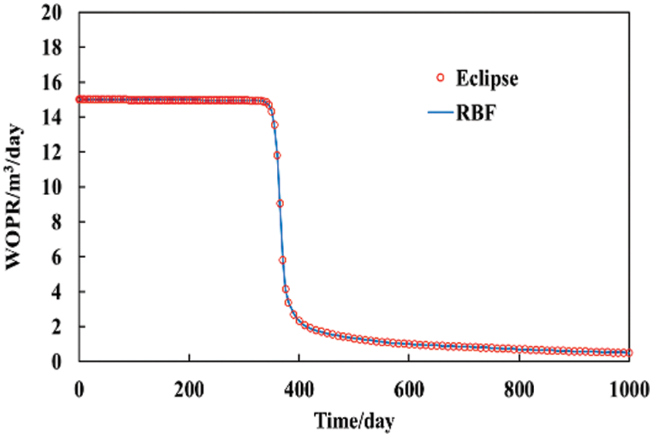
Figure 2: Daily oil production rate comparison

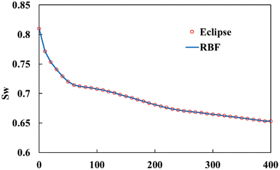
Figure 3: Water saturation at 1000 days

4  Model Application

This model is used to solve the two-dimensional reservoir flow problem. The size of the model is 200 m * 200 m * 10 m. The injection well IN1 is located at the center of the model, and the production well is located at four corners of the model. It is shown in Fig. 4. The injection rate is 200 m3/day, the recovery rate is 50 m3/day and the production time is 1000 days. The time step is Δt=10 the day, and the space step is Δx=10 m. c in the Gaussian function is 50. Some physical property information is shown in Table 1. Eclipse and finite difference method (FDM) are used to verify the accuracy of the method in this paper.

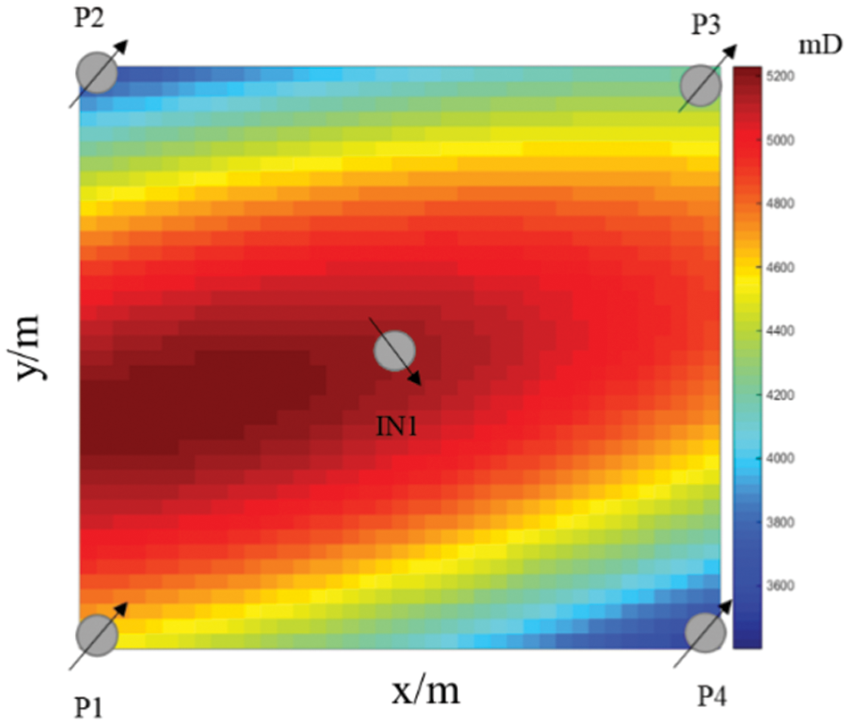
Figure 4: Two-dimensional model diagram

The permeability field plot shows that the permeability is slightly higher between P1 and IN1. In the calculation results, the water breakthrough time is 180 days for well P1, 200 days for wells P2 and P3, and 210 days for well P4. Compared with the results of the RBF and FDM, the RBF has less error and is closer to the daily oil production eclipse data, as can be seen in Fig. 5. In calculating the daily oil production data of well P1, the errors of the RBF method and the FDM method are 5.78% and 7.5%, respectively. When calculating the daily oil production of other wells, the error of the RBF method is less than 2%, and the error of the FDM method is slightly higher than that of the RBF method.

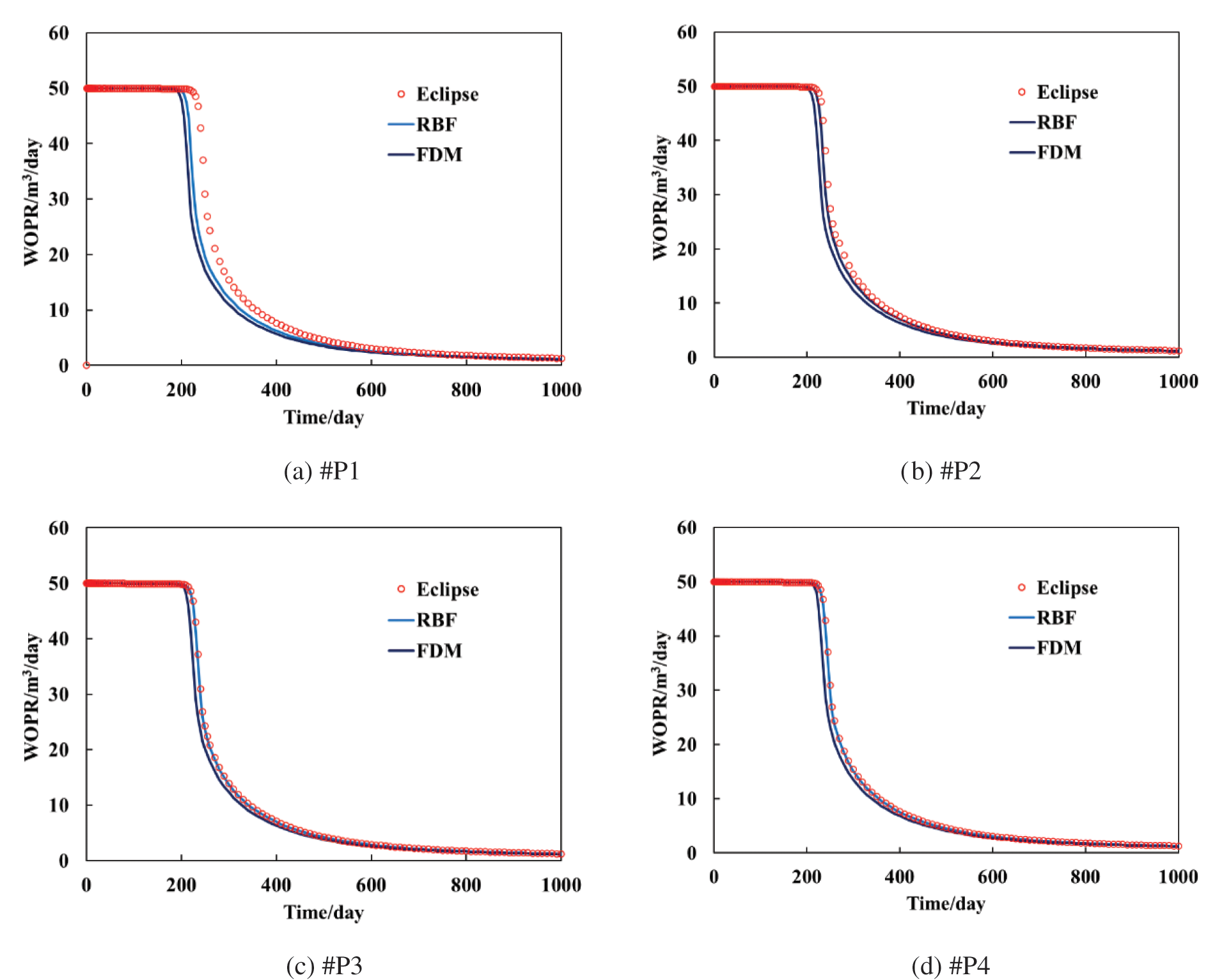
Figure 5: Daily oil production comparison of a single well

4.1 Parameter Sensitivity Analysis

Using the above two-dimensional example, this paper changes the amount of free parameter c of the Gaussian function. Select the parameters c as 30, 60, 90, and 120 for comparative calculation. The time step is Δt=10 day and the space step is Δx=10 m. Other parameters remain unchanged. The error between them and eclipse calculation results is shown in Table 2.

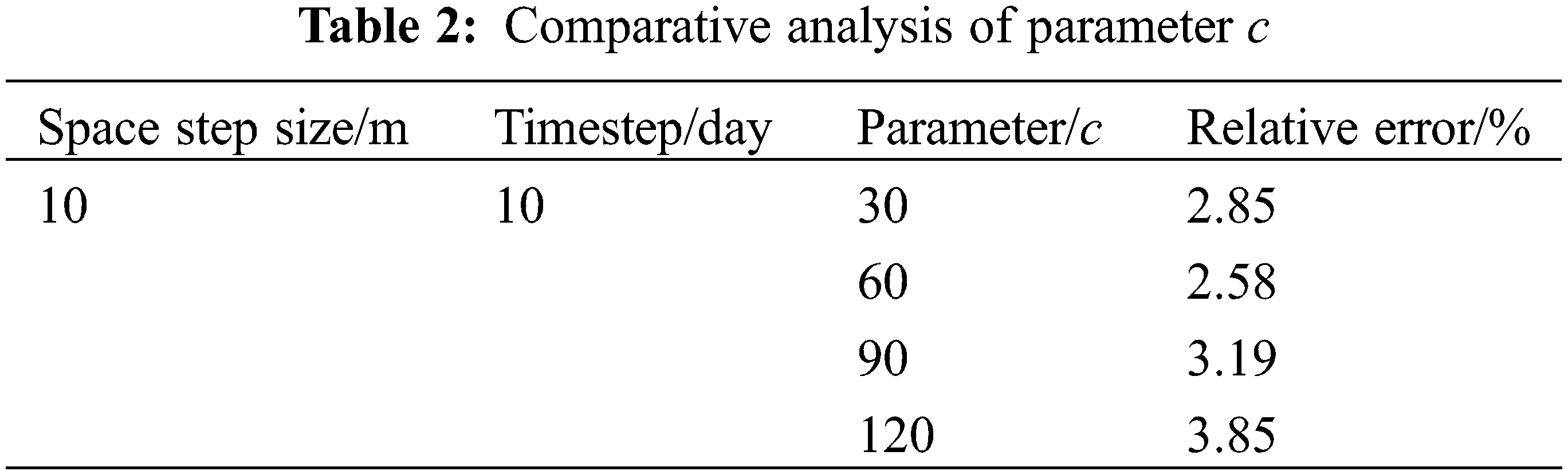
As can be seen from Table 2, the RBF is directly related to the choice of the Gaussian function parameter C. Therefore, for different problems, the appropriate parameters need to be chosen to obtain the best method.

4.2 Time Step Analysis

Using the above two-dimensional example, this paper changes the amount of time step Δt . The time steps of 5, 10, 30, and 60 days are selected for comparative calculation, the parameter c is selected as 60, and the space step is Δx=10 m. Other parameters remain unchanged. The error between them and eclipse calculation results is shown in Table 3.

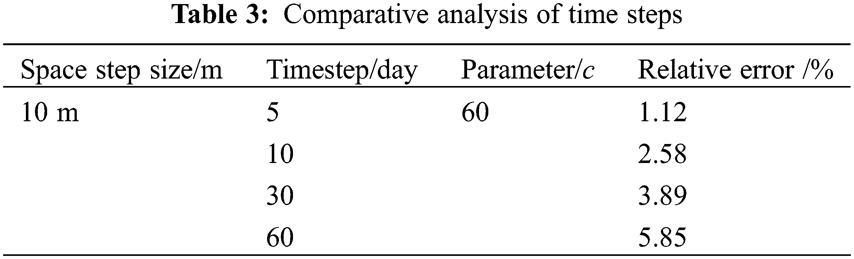
As can be seen from Table 3, the RBF method is more sensitive to the time step. Similar to other digital-analog methods, the smaller the time step, the smaller the error. It is consistent with the objective fact. When Δt is 5 days, the error is only 1.12%, but when Δt is 60 days, the error can reach 5.85%.

4.3 Space Step Analysis

Using the above two-dimensional example, this paper changes the amount of Space step size Δx . Select the space of 5, 10, 20, and 100 m for comparative calculation, the parameter c is 60, and the time step is Δt=10 the day. Other parameters remain unchanged. The error between them and eclipse calculation results is shown in Table 4.

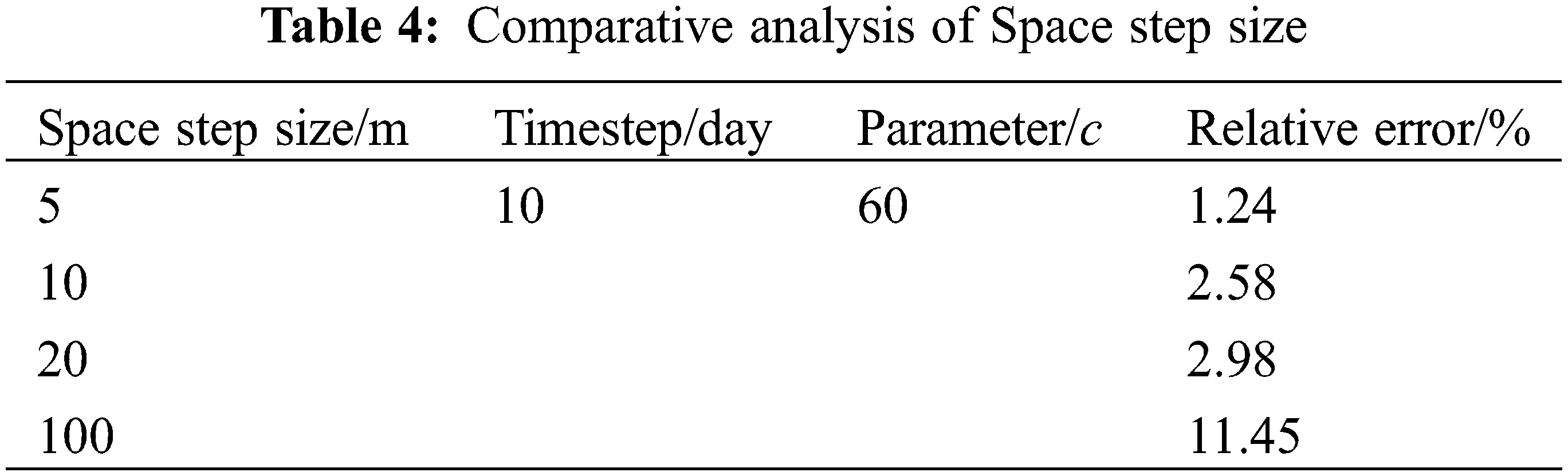
As can be seen from Table 3, the RBF has a significant sensitivity to the Space step size. Similar to other numerical simulation methods, the smaller the Space step size, the smaller the error. It is consistent with the objective fact. When Δx is 5 m, the error is only 1.24%, but when Δx is 100 m, the error can reach 11.45%.

5  Conclusion

In this paper, the radial-based meshless method is used to simulate oil-water two-phase flow in the reservoir, and relevant conclusions are obtained as follows:

(1) In this paper, the radial-based meshless method is feasible for dealing with oil-water two-phase flow in oil reservoirs. The one-dimensional example shows that the method can ensure computational accuracy, does not require meshing, is easy to implement, and saves pre-processing work compared with other methods.

(2) The two-dimensional example shows that the RBF method has a smaller error and is closer to the daily oil production eclipse data compared to the FDM method. In calculating the daily oil production data of well P1, the errors of RBF method and FDM method are 5.78% and 7.5%, respectively. When calculating the daily oil production of other wells, the error of RBF method is less than 2%, and the error of FDM method is slightly higher than that of RBF method.

(3) The computational accuracy of the radial basis function alignment meshless method is related to the radial basis function, the free parameter C and its space step and time step. One of these parameters is changed under the premise that the other parameters are determined to be constant. In this example, when the free parameter C is 60, the minimum error is 2.58%. When the spatial step is 5 meters, the minimum error is only 1.24%. When it is 5 days, the minimum error is only 1.12%.

(4) The radial basis function alignment method does not require meshing during numerical simulation and does not depend on spatial dimensions. It has the advantages of simple operation, high efficiency and high accuracy, and is suitable for solving oil-water two-phase flow problems in shale reservoirs. It overcomes the limitations of traditional methods in solving high-dimensional problems. After continuous exploration and improvement in the future, the radial basis function collocation method will be more widely used in the numerical simulation and prediction of oil-water two-phase flow in shale reservoirs.

Funding Statement: This work was supported by The China Postdoctoral Science Foundation (2021M702304) and Natural Science Foundation of Shandong Province (ZR2021QE260).

Conflicts of Interest: The authors declare that they have no conflicts of interest to report regarding the present study.

References

 1.  Zhang, J., He, S., Liu, T., Ni, T., Zhou, J. et al. (2021). Visualization of water plugging displacement with foam/gel flooding in internally heterogeneous reservoirs. Fluid Dynamics & Materials Processing, 17(5), 931–946. DOI 10.32604/fdmp.2021.015638. [Google Scholar] [CrossRef]

 2.  Zhang, X., Wang, C., Wu, H., Zhao, X. (2022). Application of new water flooding characteristic curve in the high water-cut stage of an oilfield. Fluid Dynamics & Materials Processing, 18(3), 661–677. DOI 10.32604/fdmp.2022.019486. [Google Scholar] [CrossRef]

 3.  Xu, Y., Sheng, G., Zhao, H., Hui, Y., Zhou, Y. et al. (2021). A new approach for gas-water flow simulation in multi-fractured horizontal wells of shale gas reservoirs. Journal of Petroleum Science Engineering, 199(1), 108292. DOI 10.1016/j.petrol.2020.108292. [Google Scholar] [CrossRef]

 4.  Feng, Y., Liu, Y., Chen, J., Mao, X. (2022). Simulation of the pressure-sensitive seepage fracture network in oil reservoirs with multi-group fractures. Fluid Dynamics & Materials Processing, 18(2), 395–415. DOI 10.32604/fdmp.2022.018141. [Google Scholar] [CrossRef]

 5.  Rao, X., Xu, Y., Liu, D., Liu, Y., Hu, Y. (2021). A general physics-based data-driven framework for numerical simulation and history matching of reservoirs. Advances in Geo-Energy Research, 5(4), 422–436. DOI 10.46690/ager.2021.04.07. [Google Scholar] [CrossRef]

 6.  Xu, Y., Hu, Y., Rao, X., Zhao, H., Zhong, X. et al. (2021). A fractal physics-based data-driven model for water-flooding reservoir (FlowNet-fractal). Journal of Petroleum Science Engineering, 210, 109960. [Google Scholar]

 7.  Zhou, Y., Xu, Y., Rao, X., Hu, Y., Liu, D. et al. (2021). Artificial Neural Network-(ANN) based proxy model for fast performances’ forecast and inverse schedule design of steam-flooding reservoirs. Mathematical Problems in Engineering, 2021(4), 1–12. DOI 10.1155/2021/5527259. [Google Scholar] [CrossRef]

 8.  Shaw, G., Stone, T. (2005). Finite volume methods for coupled stress/fluid flow in a commercial reservoir simulator. SPE Reservoir Simulation Symposium, The Woodlands, Texas. DOI 10.2118/93430-MS. [Google Scholar] [CrossRef]

 9.  Zhao, H., Kang, Z., Zhang, Y., Sun, H., Li, Y. et al. (2014). An interwell connectivity numerical method for geological parameter characterization and oil-water two-phase dynamic prediction. Acta Petrolei Sinica, 35(5), 922–927. DOI 10.7623/syxb201405012 [Google Scholar] [CrossRef]

10. Oñate, E., Idelsohn, S. (1998). A mesh-free finite point method for advective-diffusive transport and fluid flow problems. Computational Mechanics, 21(4–5), 283–292. DOI 10.1007/s004660050304. [Google Scholar] [CrossRef]

11. Yong, D. (2008). A note on the meshless method using radial basis functions. Computers & Mathematics with Applications, 55(1), 66–75. DOI 10.1016/j.camwa.2007.03.011. [Google Scholar] [CrossRef]

12. Zabihi, F., Saffarian, M. (2017). A not-a-knot meshless method with radial basis functions for numerical solutions of Gilson-Pickering equation. Engineering with Computers, 34(1), 37–44. DOI 10.1007/s00366-017-0519-9. [Google Scholar] [CrossRef]

13. Hardy, R. L. (1971). Multiquadric equations of topography and other irregular surfaces. Journal of Geophysical Research, 76(8), 1905–1915. DOI 10.1029/JB076i008p01905. [Google Scholar] [CrossRef]

14. Golberg, M. A., Chen, C. S., Bowman, H. (1999). Some recent results and proposals for the use of radial basis functions in the BEM. Engineering Analysis with Boundary Elements, 23(4), 285–296. DOI 10.1016/S0955-7997(98)00087-3. [Google Scholar] [CrossRef]

15. Zhang, X., Song, K. Z., Lu, M. W., Liu, X. (2000). Meshless methods based on collocation with radial basis functions. Computational Mechanics, 26(4), 333–343. DOI 10.1007/s004660000181. [Google Scholar] [CrossRef]

16. Shivanian, E. (2017). Local radial basis function interpolation method to simulate 2D fractional-time convection-diffusion-reaction equations with error analysis. Numerical Methods for Partial Differential Equations, 33(3), 974–994. DOI 10.1002/num.22135. [Google Scholar] [CrossRef]

17. Oruç, Ö. (2020). Two meshless methods based on local radial basis function and barycentric rational interpolation for solving 2D viscoelastic wave equation. Computers Mathematics with Applications, 79(12), 3272–3288. DOI 10.1016/j.camwa.2020.01.025. [Google Scholar] [CrossRef]

18. Wang Q., Yang J., Luo W. (2021). Flow simulation of a horizontal well with two types of completions in the frame of a Wellbore-Annulus–Reservoir model. Fluid Dynamics & Materials Processing, 17(1), 215–233. DOI 10.32604/fdmp.2021.011914. [Google Scholar] [CrossRef]

This work is licensed under a Creative Commons Attribution 4.0 International License, which permits unrestricted use, distribution, and reproduction in any medium, provided the original work is properly cited.