Fluid Dynamics & Materials Processing

DOI: 10.32604/fdmp.2022.021726

REVIEW

Anomaly Detection in Textured Images with a Convolutional Neural Network for Quality Control of Micrometric Woven Meshes

Pierre-Frédéric Villard1,*, Maureen Boudart2, Ioana Ilea3 and Fabien Pierre1

1Université de Lorraine CNRS Inria LORIA, Nancy, 54000, France
2IUT de Saint-Dié Université de Lorraine, Saint-Dié-des-Vosges, 88100, France
3Technical University of Cluj-Napoca, Cluj-Napoca, 400114, Romania
*Corresponding Author: Pierre-Frédéric Villard. Email: pierrefrederic.villard@loria.fr
Received: 04 February 2022; Accepted: 07 March 2022

1  Introduction

Industrial woven meshes are composed of metal material. It can be found in various industries: architecture (perforated sheets for facade cladding, railings, sunscreens, etc.), aerospace industries (engines soundproofing or air filtering and other applications including silt fence, erosion control, pipeline protection and paving products.

Defects can occur during the manufacturing process. The weaving could be altered such as having some bumps or some irregularities. It is crucial to detect them as the final product could lose its overall purpose (e.g., filtering). Companies working in industrial woven meshes have then to use a quality control process. This process is currently manually performed on sampling data. Some methods use visual observation, with a magnifying glass depending on the size. Some methods rather use the sense of touch of the employee in charge of the quality control to detect the bumps.

We propose here a method to detect such defects based on computer vision using non-geometric but textured objects. These images are opposed to natural images representing a shape such as a cat for example. We will focus on woven meshes where images do not have contours but represent a repeating pattern. One approach to identifying defects in these images will be to consider that these images are textures and that classification algorithms will be used for this purpose. The classification process is then with defect vs. without defect classes. We used a VGG19 Convolutional Neural Network (CNN). The industrial conditions of this application do not allow to have a large database. To cope with that data augmentation has been performed for the training and pre-train weights from an existing database have been used. Learning curve behaviour also had to be monitored through cross-validation. To sum up, the main objective of this work is to implement a complete framework that can automatically detect if a manufactured Micrometric Woven Mesh contain defects by using machine learning technique on a picture acquire in control conditions.

2  State of the Art

Texture represents an important aspect in visual perception, involved in objects characterization and identification. In recent years, this property has been extensively studied and used in computer vision applications, including image classification. Even though textures are easily identified and classified by human beings, they do not have a unique definition that can be used in computer vision applications. Therefore, to capture the wide variety of information lying in textures, different methods have been proposed in the literature.

For instance, textures can be characterized by statistical methods. In this case, the texture is defined by taking into consideration the spatial distribution of the contained grey values, including approaches like the grey level co-occurrence matrices [1] the autocorrelation features [2], the variograms [3,4], the local binary patterns [5], etc.

Moreover, the textural information can be extracted by using stochastic models. First, the textures are analyzed using the multiscale, or the multiresolution representation. At this point, the Fourier transform [6], the Gabor filters [7], or the wavelet transform [8] can be considered. Next, the extracted coefficients are statistically modelled, to obtain the final texture signature. The employed statistical models include the univariate generalized Gaussian distributions [9], or Gamma distributions [10]. Even though these univariate models have been successfully used for modelling filtered coefficients, they cannot consider all the information lying in images, like the spatial, or spectral dependencies. Therefore, multivariate models have been proposed, including copula-based distributions [11] spherically invariant random vectors, multivariate generalized Gaussian distributions [12], or Riemannian distributions [13].

In addition, texture can be captured through feature encoding methods which are used to model the local information contained in non-stationary images. In this case, low-level features are extracted to represent the texture information. Then a codebook is generated to identify the features containing the significant information, by using the k-means or the expectation-maximization algorithm. In the end, all the features are projected onto the codebook space.

At this stage, some of the most employed algorithms are the bag of words model [14,15], the vectors of locally aggregated descriptors [16], and the Fisher vectors [17]. First, these methods have been proposed for non-parametric features in the Euclidean space, and then they have been extended to features defined on the Riemannian manifold, given descriptors like bag of Riemannian words [18], Riemannian Fisher vectors [19], Riemannian vectors of locally aggregated descriptors [20], extrinsic vector of locally aggregated descriptors [21], etc.

Later, CNN methods have emerged in the literature. A large review has been done in [22]. In most methods, the CNN is used to produce a representation of the patches which are then used in more classic dictionary-based classification (Fisher vectors, bag of words, etc.). This combination of approaches leads to complex frameworks. In the cases studied in the literature, the texture is complex and a naive use of simple CNN methods such as VGG [23], developed by the Visual Geometry Group at the University of Oxford, would not work, which explains the complexity of the proposed approaches. In the following, we will show that in the case of very regular textures, VGG approach can achieve suitable performances.

Some deep learning approaches have been used in defect detection on fabric material. A large review can be found in [24]. For this application, (see, e.g. [25]), the state-of-the-art methods need some large database with a lot of defect samples. In fact, it is extremely difficult to provide such quantity of defect images. The method of [25] tackles this problem by generating synthetic defect images. In our work, the proposed deep learning approach performs competitive results with a small database of real defect samples.

3  Method

3.1 Database

All our database comes from an industrial context of metal woven meshes provided by our collaborating company. They are two datasets and both have been manually labelled by the quality control service of the company.

Dataset A contains images of regular grids where the defect is hardly visible to the eye. When these grids have a defect, they are not perfectly flat but they are curved. During the quality control of these grids, defects are detected by touch because it is difficult to see them with naked eyes. However, when the grids are curved, a slight difference in illumination may occur.

Dataset B contains images of grids also with a regular grid pattern. When there is a defect, there is an irregularity in the grid pattern with grid lines spaced further apart than the others.

Our approach will thus consist, for a given type of grid (types A or B), in establishing a classification model (defect vs. without defect) based on machine learning. Fig. 1 illustrates for each grid type an example of an image in each of the classes with and without defects.

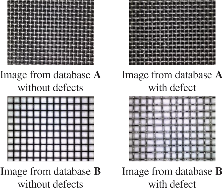
Figure 1: Example of images from both databases A and B with or without defects

3.2 CNN Architecture

A Machine learning consists in computing the parameters of a model by minimizing a cost function representing the sum of the errors associated with the model. The learning step consists of an iterative algorithm to optimize the objective function (loss) based on stochastic gradient descent. To check if the algorithm works well on our dataset, it is possible to see if the objective function decreases during the iterations. It is also possible to verify if the model can be well generalized to others data by splitting the dataset between a train and a test set and to compute the objective function on the test set while learning our model with the training set. In principle, if the algorithm works normally, during the iterations of the optimization algorithm, the accuracy increases on the training data but may not on the test data (overfitting). To visualize the correct operation of an algorithm, these values are observed during the iterations (see for example Fig. 4).

To check if a very simple CNN model could work on our data, we chose a VGG19 architecture [23], composed of 19 convolution layers. Between these convolution layers, max-pooling layers are used for regularization. As a result of these convolution layers, a dense network is activated by ReLU functions. Then there are three fully connected layers and the final layer is a softmax function. The loss function that has been used is the cross-entropy function. This configuration is among the most common ones (see Fig. 2). Since there are not enough images in the database to learn without pre-trained weights, the network learning was performed by transfer using the weights of the network trained on the ImageNet database [26]. Experiments on learning with and without pre-trained weights are presented in the Results and Discussion section. The use of a pre-trained architecture requires images with the same dimensions as the database with which it was pre-trained. So, the images were resized with a 224 × 224 bilinear interpolation. It was later refined on the database containing the grid database. Refining was carried out with Adam optimizer with a learning rate of 10−5 and batch sizes of 8. The number of epochs varies in our experiment depending on the convergence of the learning curves.

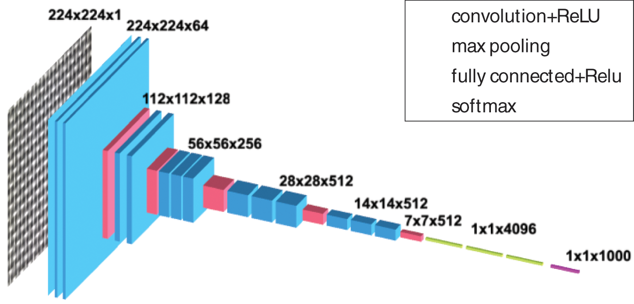
Figure 2: Architecture of the VGG19 network

3.3 Data Augmentation

The classification was initially carried out without data augmentation then with data augmentation transforming the images by rotations, translation or horizontal and vertical symmetries. The data augmentation was performed using a generator performing rotations and translations between 0 and a maximum value. Rotations from 0 to 2 degrees and from 0 to 15 degrees were tested as well as translations up to 10% of the image. Translations were performed on both horizontal and vertical axes.

In the data augmentation with translations and rotations, the missing pieces of the image resulting from the transformation were replaced by the removed parts to periodically repeat the texture of the image. An illustration of the data augmentation is given in Fig. 3.

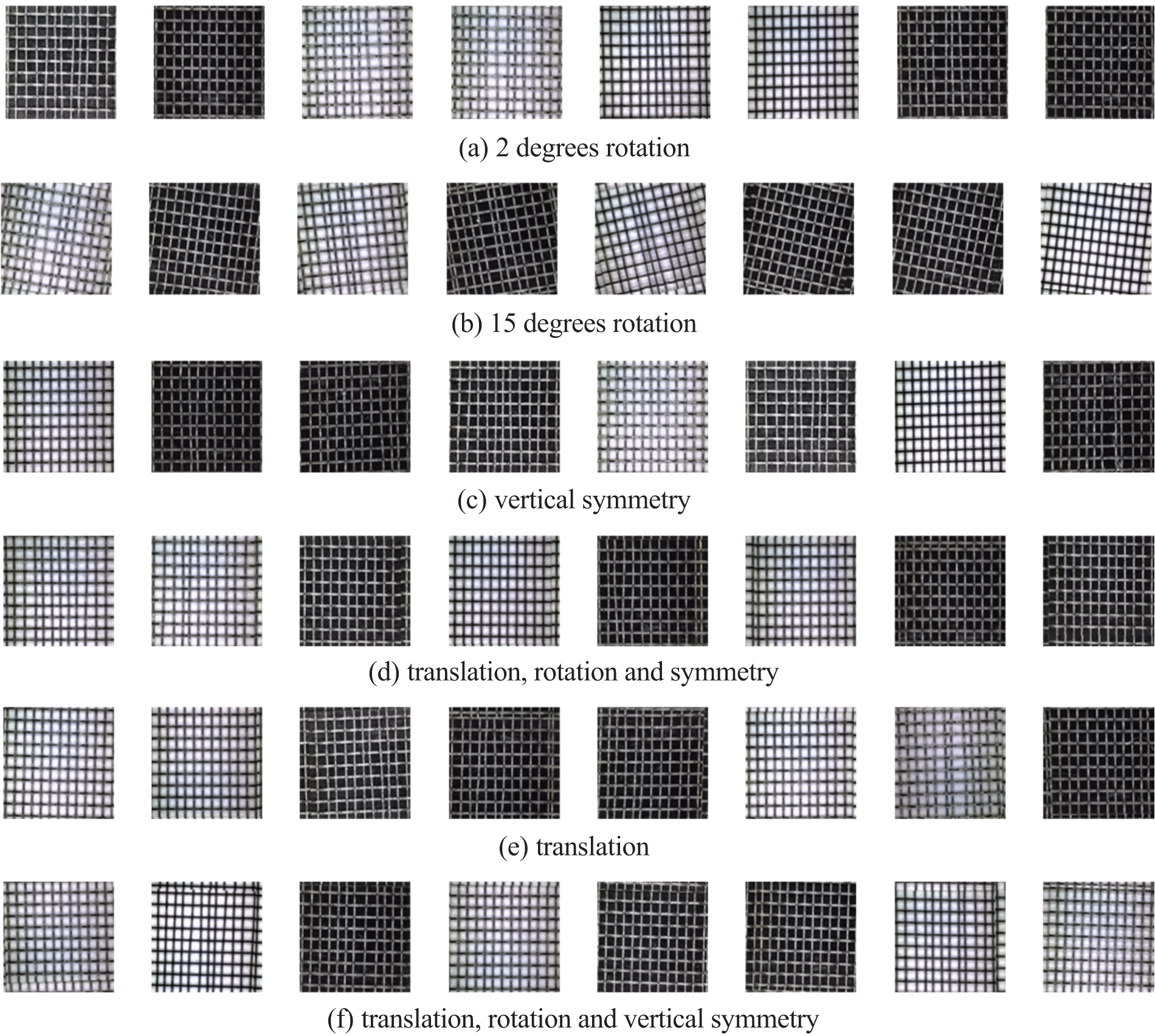
Figure 3: Example of augmented images generated on a batch of 8 images

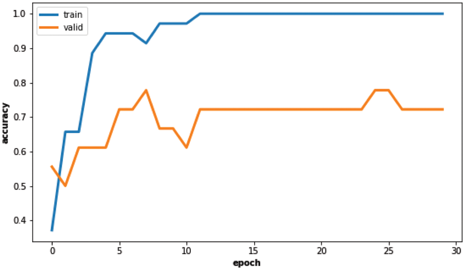
Figure 4: Dataset B learning curves without augmentation

3.4 Validation Process

To avoid over-fitting, the model was first tested on the data without pre-training to adjust the hyperparameters. The database is small, which means that a small amount of data can be used for testing. For this purpose, the cross-validation method was used with five training/test sets. The K cross-validation method consists of making K combinations of training/test sets allowing to test on a larger set of images while keeping enough images for training. The training is repeated five times (K = 5) on different data and tested on different data. The dataset was divided into five sets having 20 test images and 80 training images in each set. The validation set represents one-third of the training set. It means that we randomly select 80 data on a total of 100 to build up our prediction model and the 20 other data are used for validation. This process is repeated to be sure it is robust.

4  Results and Discussion

As previously discussed, the learning process is not efficient without using pre-trained weights and learning everything from scratch. The learning curves corresponding to this experiment is presented in Fig. 5. The curves are not stable, the accuracy is not converging toward 100% and the loss function is even not decreasing. The weights cannot be learnt on so few data without initial values closer to a reliable model.

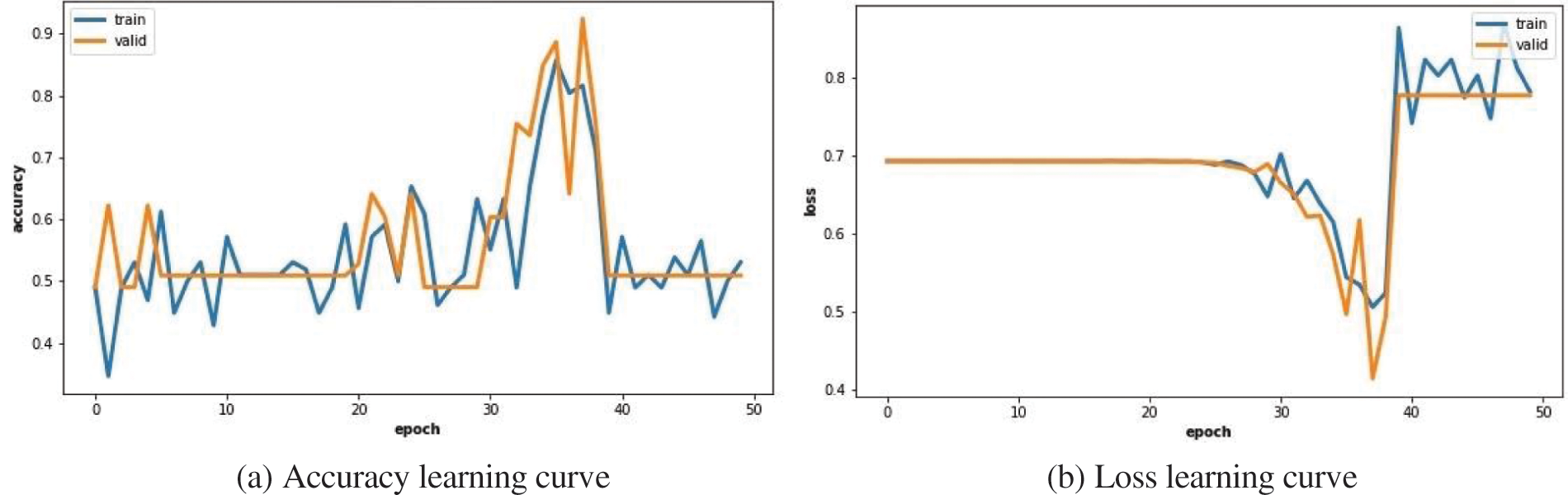
Figure 5: Learning curves on dataset B without using pre-trained weights

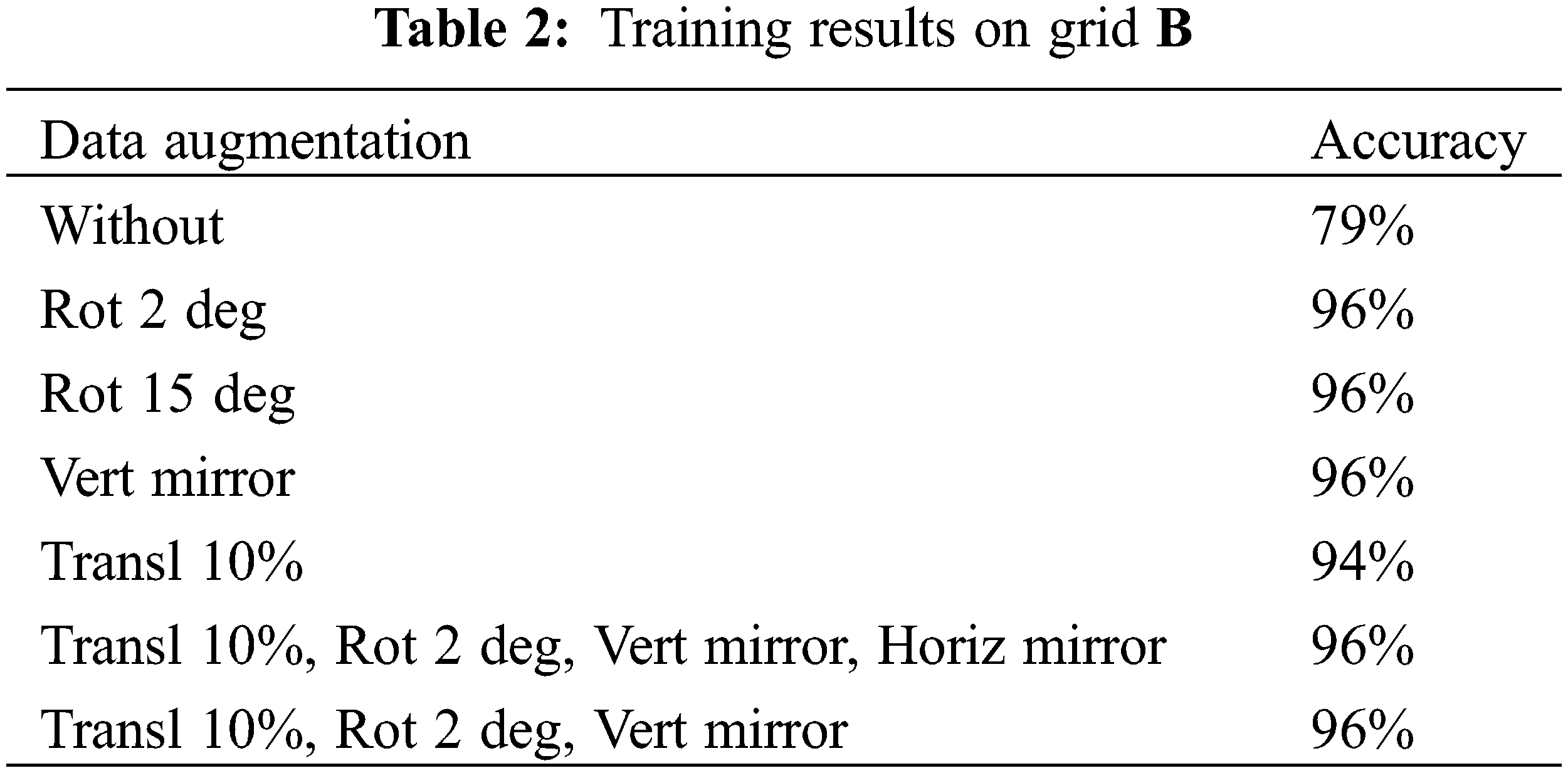
To tackle this issue, we adopt a pre-learned model and a fine-tuning is used on our dataset. With VGG19 pre-trained on imageNet we obtain an average of 15.8 correct images out of 20 representing an average precision of 79% with a variance of 3.36 (compared to the number of correct images) on the dataset B. The weights provided by imageNet are a good initialization as they represent patterns that can also occur on our dataset, like horizontal or vertical features. The accuracy of the training learning curve manages to converge to 100% but not the accuracy of the validation curve (see Fig. 4). The dataset may be probably too easy to classify and is not representative of the errors occurring in most cases of fabrication issues. Moreover, the testing set may be not large enough.

To tackle the issue of the small amount of data, we propose to use classical data augmentation techniques. When such approaches are used, only training and validation data was augmented. The accuracy of the training and the validation learning curve can converge to 100% (see Fig. 6).

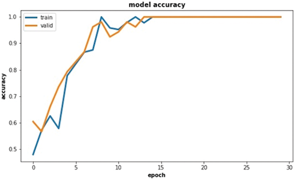
Figure 6: Accuracy learning curves on dataset B with the train (blue) and validation (orange) data when using data augmentation

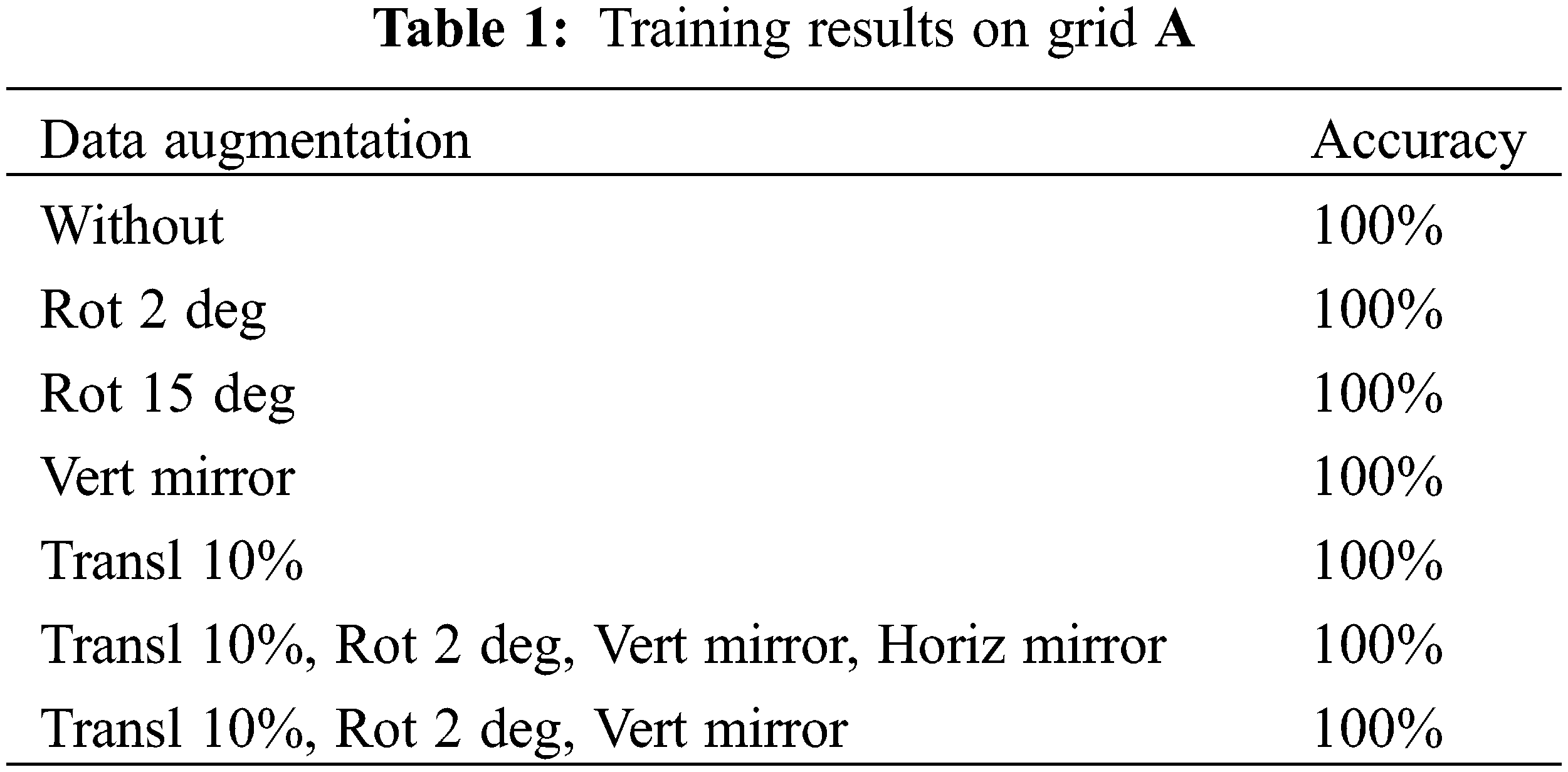
The test data are the original images with a size of 224 × 224. For each batch, the model is tested with 20 images, Tables 1 and 2 show the number of correct images for each batch. The accuracy is the average accuracy over all these batches. The data augmentation has stabilized the differences in terms of performance between the different batches, as well as the overall performance over the model. Dataset A has a score of 100% but this does not mean that the model is perfect, knowing that for each test set there are only 20 images. If the database had been larger, the 100% accuracy may not have been achieved. An error leads to a 5% drop and it is not excluded that the model would make mistakes.

Finally, the results obtained with the VGG19 architecture were compared with those obtained from the commonly used InceptionV3 architecture [27]. With this last model, 100 epochs were required to reach an acceptable convergence and the final accuracy on database B was only 90%, lower than the 96% reached with VGG19 (see Fig. 7).

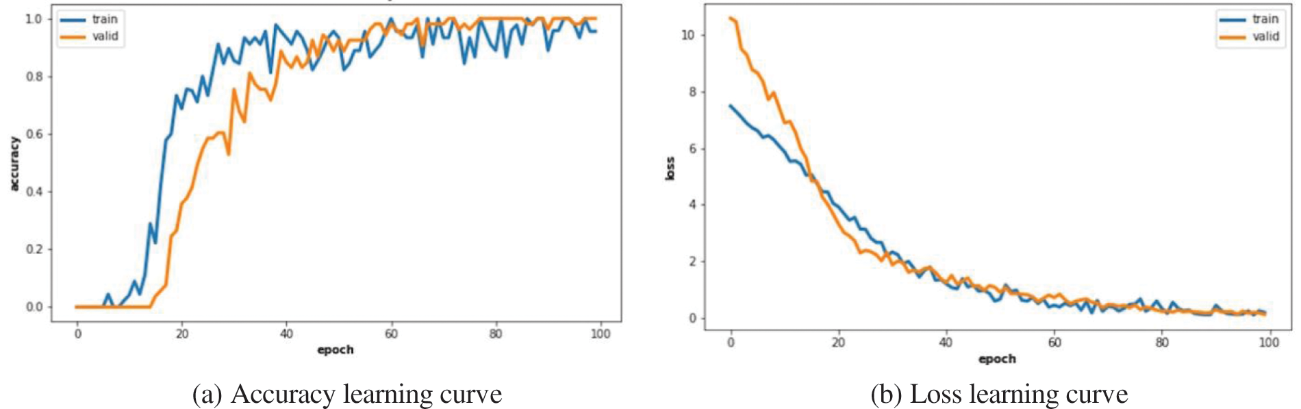
Figure 7: Learning curves on dataset A without using pre-trained weights with the train (blue) and validation (orange) data: (a) accuracy vs. epoch and (b) loss vs. epoch

As limitations of our work, two elements have to be noted: firstly, the database is too small to generalize the accuracy on the large scale and secondly only two kinds of grids have been tested. Both limitations will be addressed in future work with methods detailed in the next section.

Moreover, whereas deep learning approaches have show during the last decade a powerful prediction ability, the explanation of the results are still a open research subject (see, e.g. [28,29]) and the state-of-the-art studies are not able to give a physical interpretation of the results.

5  Conclusion

A new kind of application was presented in this paper: the direct use of CNN-based classification in the domain of micrometric industrial fabrics for quality control. This special application has the advantage of working with images acquired in a controlled environment on a material that should have a regular pattern. We show that such properties allow using much less learning data than most work of the literature with a good classification precision. We used a pre-trained VGG19 architecture and on-the-fly augmentation. In the end, we can accurately predict if there is a defect on a data from a specific metallic woven mesh with our learning process from only 80 images.

As perspectives, we plan to increase our database of industrial fabric images to check if our method could be scaled while maintaining its robust behaviour. More data is needed along with a new protocol of labelling with bounding boxes to detect localized defects. Our strategy will then be to use weak supervised networks. Another avenue of research we are considering is the generation of synthetic images of woven meshes, given the fact that everything is controlled (lighting, camera position, material, sewing patterns). In future works, we would like to develop unsupervised decision rules that can work without having a database containing samples of defects.

Acknowledgement: The authors thank the company Gantois Industries for sharing the data and the IUT of Saint-Dié-des-Vosges for funding this project.

Funding Statement: The authors received no specific funding for this study.

Conflicts of Interest: The authors declare that they have no conflicts of interest to report regarding the present study.

References

 1.  Haralick, R. M., Shanmugam, K., Dinstein, I. (1973). Textural features for image classification. IEEE Transactions on Systems, Man and Cybernetics, SMC-3(6), 610–621. DOI 10.1109/TSMC.1973.4309314. [Google Scholar] [CrossRef]

 2.  Tuceryan, M., Jain, A. K. (1993). Texture analysis. In: Handbook of pattern recognition and computer vision, pp. 235–276. DOI 10.1142/1802. [Google Scholar] [CrossRef]

 3.  Matheron, G. (1963). Principles of geostatistics. Economic Geology, 58(8), 1246–1266. [Google Scholar]

 4.  Curran, P. J. (1988). The semi variogram in remote sensing: An introduction. Remote Sensing of Environment, 24(3), 493–507. DOI 10.1016/0034-4257(88)90021-1. [Google Scholar] [CrossRef]

 5.  Ojala, T., Pietikainen, M., Harwood, D. (1996). A comparative study of texture measures with classification based on feature distributions. Pattern Recognition, 29(1), 51–59. DOI 10.1016/0031-3203(95)00067-4. [Google Scholar] [CrossRef]

 6.  Georgeson, M. A. (1979). Spatial Fourier analysis and human vision. Tutorial Essays in Psychology, 2, 39–88. DOI 10.1007/978-3-319-25040-3_40. [Google Scholar] [CrossRef]

 7.  Turner, M. R., (1986). Texture discrimination by gabor functions. Biological Cybernetics, 55(2–3), 71–82. DOI 10.1007/BF00341922. [Google Scholar] [CrossRef]

 8.  Mallat, S. G. (1989). A theory for multiresolution signal decomposition: The wavelet representation. IEEE Transactions on Pattern Analysis and Machine Intelligence, 11(7), 674–693. DOI 10.1109/34.192463. [Google Scholar] [CrossRef]

 9.  Do, M. N., Vetterli, M. (2002). Wavelet-based texture retrieval using generalized Gaussian density and kullback-leibler distance. IEEE Transactions on Image Processing, 11, 146–158. DOI 10.1109/83.982822. [Google Scholar] [CrossRef]

10. Mathiassen, J., Skavhaug, A., Bø, K. (2002). Texture similarity measure using kullback-leibler divergence between gamma distributions. Proceedings of the 7th European Conference on Computer Vision–Part III, pp. 133–147. UK. [Google Scholar]

11. Lasmar, N. E., Berthoumieu, Y. (2014). Gaussian copula multivariate modeling for texture image retrieval using wavelet transforms. IEEE Transactions on Image Processing, 23(5), 2246–2261. DOI 10.1109/TIP.2014.2313232. [Google Scholar] [CrossRef]

12. Pascal, F., Bombrun, L., Tourneret, J. Y., Berthoumieu, Y. (2013). Parameter estimation for multivariate generalized Gaussian distributions. IEEE Transactions on Signal Processing, 61(23), 5960–5971. DOI 10.1109/TSP.2013.2282909. [Google Scholar] [CrossRef]

13. Said, S., Bombrun, L., Berthoumieu, Y. (2015). Texture classification using Rao’s distance on the space of covariance matrices. In: Geometric science of information. Paris, France. [Google Scholar]

14. Lazebnik, S., Schmid, C., Ponce, J. (2005). A sparse texture representation using local affine regions. IEEE Transactions on Pattern Analysis and Machine Intelligence, 27(8), 1265–1278. DOI 10.1109/TPAMI.2005.151. [Google Scholar] [CrossRef]

15. Varma, M., Zisserman, A. (2004). A statistical approach to texture classification from single images. International Journal of Computer Vision, 62, 61–81. DOI 10.1007/s11263-005-4635-4. [Google Scholar] [CrossRef]

16. Cimpoi, M., Maji, S., Kokkinos, I., Mohamed, S., Vedaldi, A. (2013). Describing textures in the wild. IEEE Conference on Computer Vision and Pattern Recognition, Greater Columbus Convention Center in Columbus, Ohio, USA. [Google Scholar]

17. Sanchez, J., Perronnin, F., Mensink, T., Verbeek, J. (2013). Image classification with the fisher vector: Theory and practice. International Journal of Computer Vision, 105(3), 222–245. DOI 10.1007/s11263-013-0636-x. [Google Scholar] [CrossRef]

18. Faraki, M., Harandi, M. T., Wiliem, A., Lovell, B. C. (2014). Fisher tensors for classifying human epithelial cells. Pattern Recognition, 47(7), 2348–2359. DOI 10.1016/j.patcog.2013.10.011. [Google Scholar] [CrossRef]

19. Ilea, I., Bombrun, L., Germain, C., Terebes, R., Borda, M. et al. (2016). Texture image classification with riemannian fisher vectors. IEEE International Conference on Image Processing, pp. 3543–3547. Phoenix, AZ, USA. [Google Scholar]

20. Faraki, M., Harandi, M. T., Porikli, F. (2015). More about VLAD: A leap from Euclidean to riemannian manifolds. IEEE Conference on Computer Vision and Pattern Recognition, pp. 4951–4960. Boston, USA. [Google Scholar]

21. Faraki, M., Harandi, M., Porikli, F. (2015). Material classification on symmetric positive definite manifolds. IEEE Winter Conference on Applications of Computer Vision, pp. 749–756. Big Island, USA. [Google Scholar]

22. Liu, L., Chen, J., Fieguth, P., Zhao, G., Chellappa, R. et al. (2019). From BoW to CNN: Two decades of texture representation for texture classification. International Journal of Computer Vision, 127(1), 74–109. DOI 10.1007/s11263-018-1125-z. [Google Scholar] [CrossRef]

23. Simonyan, K., Zisserman, A. (2014). Very deep convolutional networks for large-scale image recognition. arXiv: 1409.1556. [Google Scholar]

24. Rasheed, A., Zafar, B., Rasheed, A., Ali, N., Sajid, M. et al. (2020). Fabric defect detection using computer vision techniques: A comprehensive review. Mathematical Problems in Engineering, 1–24. DOI 10.1155/2020/8189403. [Google Scholar] [CrossRef]

25. Han, Y. J., Yu, H. J. (2020). Fabric defect detection system using stacked convolutional denoising auto-encoders trained with synthetic defect data. Applied Sciences, 10(7), 2511. DOI 10.3390/app10072511. [Google Scholar] [CrossRef]

26. Deng, J., Dong, W., Socher, R., Li, L. J., Li, K. et al. (2009). ImageNet: A large-scale hierarchical image database. IEEE Conference on Computer Vision and Pattern Recognition, pp. 248–255. Miami, FL, USA. [Google Scholar]

27. Szegedy, C., Vanhoucke, V., Ioffe, S., Shlens, J., Wojna, Z. (2015). Rethinking the inception architecture for computer vision. Proceedings of the IEEE Conference on Computer Vision and Pattern Recognition (CVPR), pp. 2818–2826. [Google Scholar]

28. Pope, P. E., Kolouri, S., Rostami, M., Martin, C. E., Hoffmann, H. (2019). Explainability methods for graph convolutional neural networks. Proceedings of the IEEE/CVF Conference on Computer Vision and Pattern Recognition, pp. 10772–10781. Long Beach, CA, USA. [Google Scholar]

29. Yuan, H., Yu, H., Gui, S., Ji, S. (2012). Explainability in graph neural networks: A taxonomic survey. arXiv:2012.15445. [Google Scholar]

This work is licensed under a Creative Commons Attribution 4.0 International License, which permits unrestricted use, distribution, and reproduction in any medium, provided the original work is properly cited.