| Fluid Dynamics & Materials Processing |
DOI: 10.32604/fdmp.2022.022047
ARTICLE
Modeling the Unsteady Flow of a Newtonian Fluid Originating from the Hole of an Open Cylindrical Reservoir
1Laboratory of Mechanics Energetic and Environment (LMEE), University of Fianarantsoa, Fianarantsoa, B.P.1264, Madagascar
2Laboratory of Mathematics and Physics (LA.M.P.S), University of Perpignan Via Domitia, Perpignan, 66860, France
*Corresponding Author: Andrianantenaina Marcelin Hajamalala. Email: hajamalalaa@yahoo.fr
Received: 18 February 2022; Accepted: 23 March 2022
Abstract: This work deals with the modeling of the unsteady Newtonian fluid flow associated with an open cylindrical reservoir. This reservoir presents a hole on the right bottom wall. Fluid volume variation, heat and mass transfers are neglected. The unsteady governing equations are based on the conservation of mass and momentum. A finite volume technique is used to solve the non-dimensional equations and related boundary conditions. The algebraic system of equations resulting from the discretization process are solved by means of the THOMAS algorithm. For pressure-velocity coupling, the SIMPLE algorithm (Semi Implicit Method for Pressure Linked Equations) is used. Results for laminar flow (Re < 1000), including the pressure and velocities profiles as well as the streamlines in the reservoir are presented. Moreover, the effects of the D/d and H0/D ratios and Reynolds number Re on the fluid flow are discussed. It is shown that the velocities and pressure depend essentially on the reservoir size. To validate the model, the present results have been compared with Zhou et al.’s results, Poiseuille’s and Bernoulli’s exact solution.
Keywords: Modeling; newtonian fluid; cylindrical reservoir; navier-stokes
Nomenclature
| d | Hole diameter [m] |
| d+ | Dimensionless hole diameter = d/d |
| D | Reservoir diameter [m] |
| Fr | Froude number |
| g | Gravity acceleration [m.s−2] |
| H0 | Reservoir height [m] |
| P | Total pressure [Pa] |
| P+ | Dimensionless pressure |
| P0 | Atmospheric pressure [Pa] |
| r | Radial coordinate [m] |
| r+ | Dimensionless radial coordinate = r/d |
| Re | Reynolds number = ρU0d/μ |
| t | Time [s] |
| t+ | Dimensionless time = U0t/d |
| tf | Maximal time [s] |
| | Dimensionless maximal time |
| U0 | Average fluid velocity at outlet [m.s−1] |
| u | Fluid velocity following z [m.s−1] |
| u+ | Dimensionless fluid velocity following z+ = u/U0 |
| v | Fluid velocity following r [m.s−1] |
| v+ | Dimensionless fluid velocity following r+ = v/U0 |
| z | Axial coordinate [m] |
| z+ | Dimensionless axial coordinate = z/d |
| ρ | Fluid density [kg.m−3] |
| μ | Dynamic viscosity of the fluid [kg.m−1.s−1] |
| υ | Kinematic viscosity of the fluid [m2.s−1] |
The reservoir has a very important role in industry applications. It is presented in different forms. It is considering here the open cylindrical form. The researchers generally focus their studies on the emptying of open cylindrical tank through an orifice centered on the bottom. In a drain, the fluid height decreases with the time and the orifice size [1].
The fluid has two types draining single-layer and double-layer. Zhou et al. [2] developed numerically the single-layer flow of an open cylindrical tank with an orifice placed symmetrically on the bottom. They found a synchronization of the critical heights calculated with the analytical solution of Lubin et al. [3]. For fluids having different densities, the double-layer flow has been studied experimentally by Forbes et al. [4]. When the orifice is open, the liquid flows and the dip forms on the liquid surface in the tank.
To determine the time of fluid drain, Fadhilah et al. [5] studied the numerical simulation of the liquid flow in a cylindrical tank using open FOAM.
The numerical simulation of free surface flow in the reservoir has been studied by Xhang et al. [6]. They modeled theirs system using Navier-Stokes equation and unstructured finite volume method. Authors considered that the walls are rigid or elastic and that the fluids are viscous or not. They simulated also the viscous fluid flow past a submerged obstacle in the reservoir.
Knowing the exact emptying time of vessel is very important because it gives an advantage to plan the work and permits to anticipate all the risks caused by the lost time. For this reason, Nasyrova et al. [7] were interested in numerical study to compare the theoretical model and real tank. The purpose of this work is to demonstrate Torricelli’s law for reservoirs having the same size but a different geometry. The determination of time draining is based on the discrete element method assuming that the fluid is multiphase (gas-liquid).
Peng et al. [8] modeled fluid flow in rectangular shallow basins by using lattice Boltzmann method. They studied the system under the different conditions and basin geometry. The governing equations are those that govern sallow water. To solve these equations, the semi Lagrangian method is used. Their results showed that the proposed model is acceptable for modeling shallow basin.
To be able to supply water drinkable in urban environment with a low investment cost, Camnasio et al. [9] analyzed the coupling between flow and sediment deposition in rectangular shallow reservoir. The obtained results confirmed the existence of sedimentation that resulted in the formation of vortex inside the reservoir.
The purpose of Kalyan et al.’s [10] researches is to analyze the water flow tank using nonlinear finite element. Navier-Stokes equations have been used to model their system. They assumed that water is compressible and is discretized eight nodes. The study is carried out the hydrodynamic pressure. For various tank lengths, the nonlinear influences are also developed.
The work of Memon et al. [11] was focused on determination of exact solution for unsteady tank drainage through the circular pipe. They supposed that the fluid is incompressible and Newtonian, the couple stress is isotherm. The exact solution is obtained from governing equation (continuity and momentum) to determine the time for complete drainage.
This article presents the concept of applying numerical model to study the unsteady 2D fluid flow in cylindrical reservoir with a hole based on the Navier-Stockes equations by analyzing the influences of the more important parameters on the velocities and pressure as the Reynolds number and the configuration parameters. The lack of work on the flow characterizing this configuration motivated us to carry out this research. In this work, governing equations are resolved using the finite volume method based on Thomas algorithm. Fluid volume variation, heat and mass transfer are neglected in this case. The tank configuration and flow parameters influence on the pressure and the velocity profiles as well as the streamlines profile in the tank are investigated.
Fig. 1 shows the physical description of the system. It is composed of an open cylindrical reservoir filled with water and a hole placed on the right bottom wall. The height and diameter of the reservoir are H0 and D respectively whereas the hole diameter is d.

Figure 1: Geometrical configuration
The system in Fig. 1 has been considered. The flow is supposed two-dimensional, laminar and incompressible. Heat and mass transfers are neglected. The fluid level and the physical properties are assumed to be constant. The gravity force exerts only on this fluid. With respect of mentioned assumptions and after introducing the dimensionless transformation, the dimensionless Navier Stokes equations in cylindrical coordinate is written as follows [12]:
Dimensionless continuity equation:
Dimensionless momentum equation:
Reynolds and Froude numbers:
Dimensionless boundary conditions:
At the reservoir outlet:
At the reservoir inlet:
On the walls:
The discretization of the dimensionless Navier Stokes equations as mentioned above using the finite volume method leads to the following general form [13]:
With ϕ = (u+, v+, P+)
The SIMPLE and Thomas algorithms have been used to solve respectively the pressure-velocity coupling and the algebraic equations system has been solved by THOMAS algorithm [14], see Eq. (8).
For the numerical simulation, the reservoir data illustrated in the Table 1 below is used.

Based on the analyzes of the influence of the meshes on the results, the mesh 70 × 30 nodes was chosen to save run time and memory for numerical computation.
The convergence criterion is determined such that the source term of pressure correction equation is less than 10−8.
3.1 Profiles of Dimensionless Components of Velocities
Fig. 2 illustrates the variation in z+ = 7.5 of the adimensional speed u+ according to r+ for three durations: t+ = 7.9, 5.26 and 2.63. It should be noted that a component of the negative velocity reflects a descending flow, the highest absolute value of which is located at the vicinity of the hole of the reservoir. The inflection point observed near the left vertical wall results from the boundary conditions at the free water surface that one have imposed on the velocity. The dimensionless u+ is an increasing function of dimensionless time t+ and it will become constant until a certain time, which is the establishment time. The profile stops changing, which is to say the flow has become stationary. The unsteady flow at the beginning and the peak of adimensional velocity are caused by the existence of the orifice on the right bottom wall.

Figure 2: Effect of t+ with adimensional velocity u+
The evolution in z+ = 7.5 of the adimensional velocity component v+ according to r+ describes a parabolic profile characteristic of a Poiseuille flow, see Fig. 3. The speed v+ increases with time t+. The adimensional velocities u+ and v+ have an opposite directions. In this case, we have a Poiseuille’s profile. By moving away from the wall, the shear stress is less important and the fluid can flow freely. In accordance with the u+ speed, the destabilization of the flow begins at the inlet of the hole and becomes more and more stable.

Figure 3: Effect of t+ on the adimensional velocity v+
3.2 Profile of the Dimensionless Pressure P+
By taking three values of t+; z+ = 7.5; Fr = 0.1 and Re = 100, the dimensionless pressure profile as a function of r+ is given by Fig. 4. It is observed that the three curves are confounded. This means that the pressure always remains constant inside the tank. It is independent of time.

Figure 4: Influence of t+ on dimensionless pressure P+
3.3 Influences of the Reynolds Number on u+, v+ and P+
The Reynolds number Re is based on the average speed of water at the reservoir outlet. The increasing of the Reynolds number means that the velocity in the tank is intensifying. Fig. 5 shows the effect of Re on dimensionless velocity u+ for z+ = 7.5, t+ = 5 and Fr = 0.1. The Reynolds number and velocity u+ grow proportionally. The hole at the bottom causes the pic on the velocity u+, see Fig. 5.

Figure 5: Influence of reynolds number on velocity u+
Fig. 6 represents the influences of Reynolds number Re on adimensional velocity v+ for z+ = 7.5, t+ = 5, Fr = 0.1. According to the figure, Reynolds number Re and the adimensional velocity v+ progress regularly. For low Reynolds number Re, a parabolic profile of the boundary layer type was obtained. Otherwise, the curve gradually deviates from the other curves corresponding to the low Reynold value. The parabolic profile slowly disappears. The regime tends towards a turbulent regime. The speed v+ varies according to the evolution of the Reynolds number.
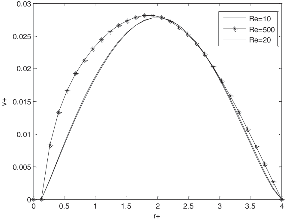
Figure 6: Influence of reynolds number on velocity v+
For various Re, Fig. 7 represents the dimensionless pressure profile as a function of r+ at x+ = 10, t+ = 100, Fr = 6.32. Even if the Reynolds number Re is varied, the pressure in the reservoir remains always almost unchanged. Therefore, Re has a small influence on the pressure P+.

Figure 7: Influence of reynolds number on pressure P+
The H0/D ratio considerably influences the evolution in z+ = 7.5 of the speed component u+ according to radial component r+, see Fig. 8 below. In fact, the increase in this ratio results in a disappearance of the inflection point observed in the vicinity of the outlet orifice and by a decrease in the absolute value of this dimensionless speed component which is all the greater as the ratio H0/D is high. In fact, the increase in the H0/D ratio generates, for a given length of the reservoir, an increase in the height of the water column and consequently in the speed of ejection of the water at the outlet of the orifice. In fact, the velocity profile u+ continuously deforms along the height of the tank and tends towards a parabolic profile.
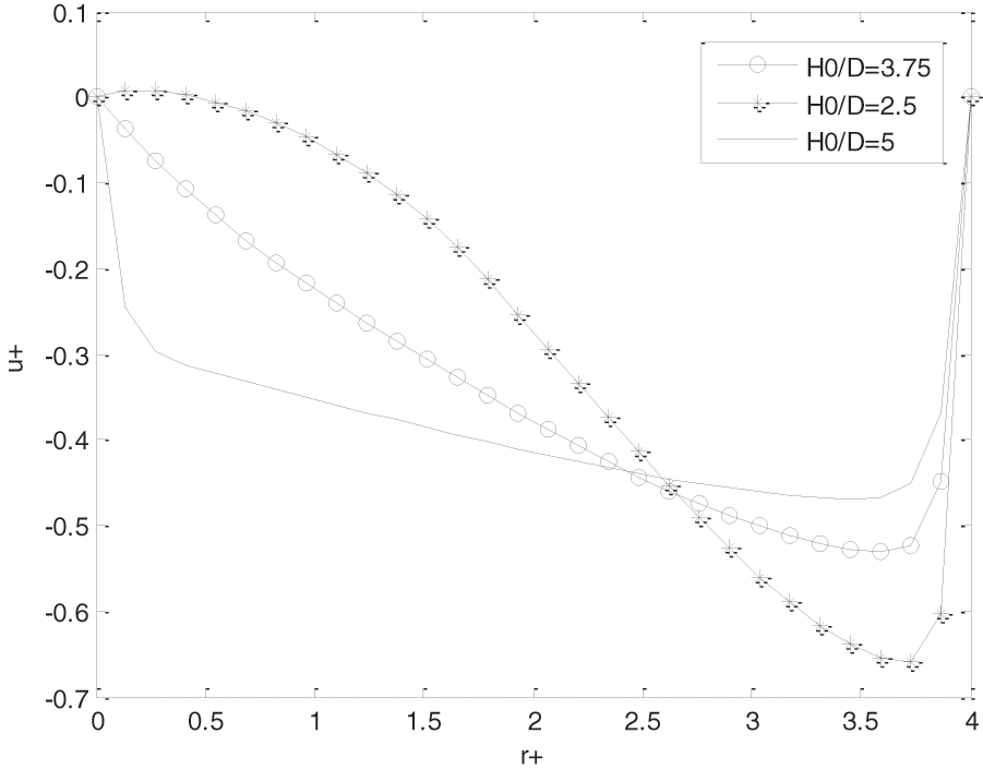
Figure 8: Influence of the variation of the ratio H0/D ratio
3.5 Influence of Orifice Diameter Variation
The D/d ratio considerably influences in z+ = 7.5 the evolution of adimensional speed component u+ according to r+ depicted in Fig. 9. The increase in the D/d ratio, for a value of d, results in a reduction in the size of the outlet orifice of the reservoir and consequently in the hydraulic diameter and therefore in the Reynolds number. This results in an increase in the transfer of momentum by diffusion to the detriment of convection. The maximum value is obtained for values of r+ close to the opening of the reservoir. These three curves are similar. If the ratio of D/d is small, D and d have comparable sizes, the fluid flows freely and its speed becomes very important. Orifice diameter d very small, in front D corresponds to the very large D/d value causes the braking of the flow near the hole.

Figure 9: Influence of the opening of the orifice
Fig. 10 shows the trajectories of the fluid particles (streamlines) in the tank at t+ = 2.63; Fr = 0.1; Re = 100. One proved from this figure that under the action of the gravity field the fluids converge towards the discharge hole.

Figure 10: Streamline in the reservoir
3.7.1 Validation with Zhou et al. Results [2]
To validate our model, the results of Zhou et al. [2] have been used. In this case, the hole of dimensionless diameter d+ = 0.2 must place in the center of the tank and one have taken Re = 100; Fr = 1; H0/D = 1; r+ = 1 and t+ = 1.2.
The profile of curves on Fig. 11 represents the comparison between Zhou et al. results [2] and the present results. One proves that the discrepancy between these two models is of the order of 1.43% on average.

Figure 11: Comparison between Zhou et al. results [2] and the present numerical results
3.7.2 Validation with Analytical Result
By changing the diameter d of the orifice to the diameter D of the tank (d = D), our system can be assimilated as a vertical cylindrical pipe. This condition has been used to validate our model. The present result has been compared with Poiseuille’s result. Fig. 12 affirms that the two curves have almost same appearance. The accuracy of model is of 97%. Comparison presents a good agreement.

Figure 12: Comparison between the analytic results and the present numerical results
3.7.3 Validation with Bernoulli’s Exact Solution
The one-dimensional unsteady Bernoulli equation was used to validate our results. By integrating this equation along the streamlines, the adimensional analytical expression is given by Eq. (9) [15].
To be able to compare the present result with that of Bernoulli, the orifice has been placed symmetrically at the reservoir’s bottom and it has been assumed that the flow is one-dimensional, that is to say that the variation of the speed is neglected along the direction r.
These two curves in Fig. 13 represent respectively the variation of adimensional velocity average depending of the adimensional time t+ for the present study and the Bernoulli’s exact solution. Results comparisons show a good agreement with a discrepancy of 2% in average.
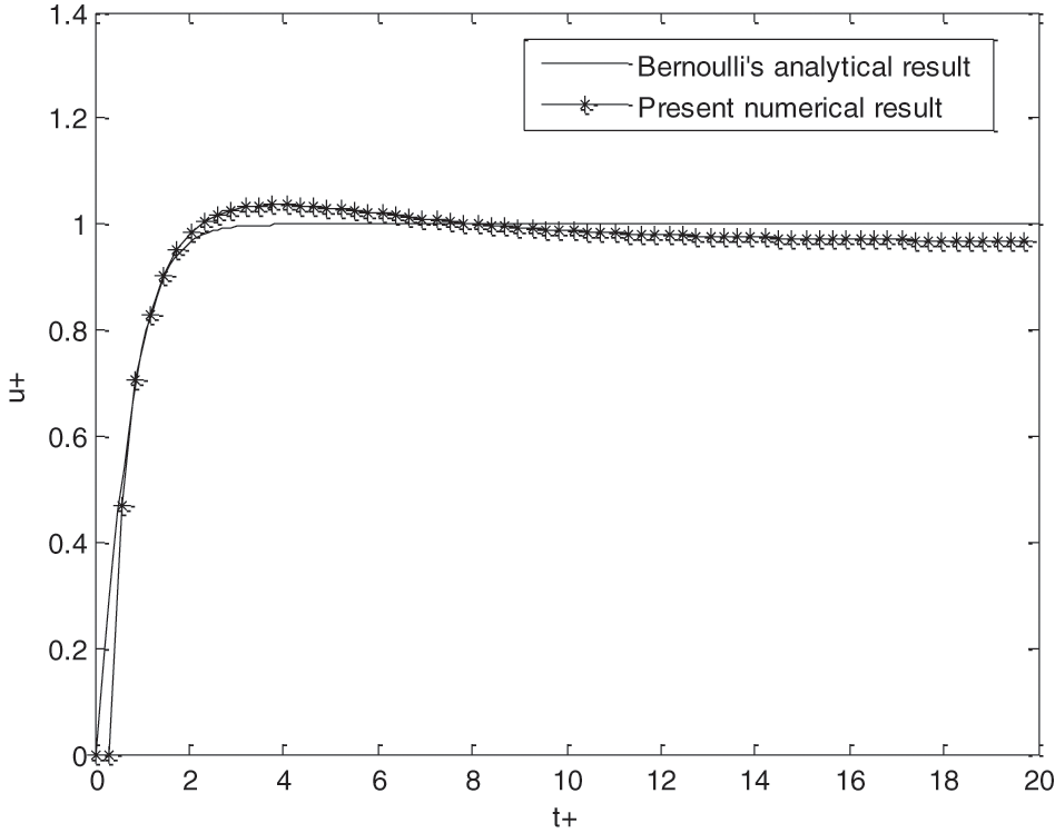
Figure 13: Validation with Bernoulli’s analytical result
A 2D model has been developed to simulate the unsteady flow. The mathematical model is based on the mass conservation and momentum. It was assumed that there are no heat and mass transfers. The governing equations and the boundary conditions were discretized using the finite volume method. The solution of the algebraic equations system is assured by Thomas’s algorithm. The SIMPLE algorithm has been used to solve the pressure-velocity coupling. The results show us the influences of t+, H0/d, D/d, Re on the velocities (u+, v+) and the pressure. Comparisons between the present results and from those literatures were done and present a good agreement. The following conclusions are drawn:
(1) The existence of the orifice on the bottom wall causes the rapid increase (peak) of the adimensional velocity and the instability of the flow at the beginning. By moving away from the wall, the shear stress is less important and the fluid can flow freely. In accordance with the velocity u+, the destabilization of the flow begins at the inlet of the hole and becomes more and more stable.
(2) The dimensionless velocities increase proportionally with the Reynolds number. For low Reynolds number, a parabolic profile of the boundary layer type was obtained. Otherwise, the regime tends towards a turbulent regime. The pressure always remains constant inside the tank. It is independent of time.
(3) The speed of ejection of the water at the outlet of the orifice increase proportionally with height of the water column. The velocity profile u+ continuously deforms along the height of the tank and tends towards a parabolic profile.
(4) The transfer of momentum by diffusion to the detriment of convection decrease with increase of the orifice diameter. The small value of orifice diameter causes the braking of the flow near the hole.
The continuity of this work concerns the experimental validation of the obtained theoretical results, the numerical study for turbulent or laminar flow in the same tank with or without obstacle by considering the heat and mass transfer at the reservoir wall.
Acknowledgement: Thanks to the team of the Laboratory of Mechanics Energetic and Environment (LMEE) for their collaboration.
Funding Statement: The authors received no specific funding for this study.
Conflicts of Interest: The authors declare that they have no conflicts of interest to report regarding the present study.
1. Yuce, M. I., Chen, D. (2003). An experimental investigation of pollutant mixing and trapping in shallow coastal recirculating flows. Proceeding of the International Symposium on Shallow Flows, vol. 4, pp. 413–420. London. [Google Scholar]
2. Zhou, Q. N., Graebel, W. P. (1990). Axisymmetric draining of a cylindrical tank with a free surface. Journal of Fluid Mechanic, 221, 511–532. DOI 10.1017/S0022112090003652. [Google Scholar] [CrossRef]
3. Lubin, B. T., Springer, G. S. (1967). The formation of a dip on the surface of liquid draining from a tank. Journal of Fluid Mechanic, 29, 385–390. DOI 10.1016/j.apm.2010.03.032. [Google Scholar] [CrossRef]
4. Forbes, L. K., Hocking, G. C. (2010). Unsteady flow of a fluid from a circular tank. Applied Mathematical Modelling, 34, 3958–3975. DOI 10.1017/S0022112067000898. [Google Scholar] [CrossRef]
5. Fadhilah, M. S., Sakri, M., Zaki, M. S., Salime, S. (2017). Numerical simulation of liquid draining from a tank using openFOAM. Materials Science and Engineering, 226(1), 012152. DOI 10.1088/1757-899X/226/1/012152. [Google Scholar] [CrossRef]
6. Zhang, X., Sudharsan, N. M., Ajaykumar, R., Kumar, K. (2005). Simulation of free surface flow in a tank using the navier-stokes model and unstructured finite volume method. Journal of Mechanical Engineering Science, 21, 203–210. DOI 10.1243/095440605X8496. [Google Scholar] [CrossRef]
7. Nasyrova, M. I., Kulakov, P. A. (2019). Numerical simulation of a draining vessel. Journal of Physics, 1384, 1–8. DOI 10.1088/1742-6596/1384/1/012033. [Google Scholar] [CrossRef]
8. Peng, Y., Zhou, J. G., Burrows, R. (2011). Modeling free-surface flow in rectangular shallow basins by using lattice Boltzmann method. Journal of Hydraulic Engineering, 137, 1680–1685. DOI 10.1061/(ASCE) HY.1943.7900.0000470. [Google Scholar]
9. Camnasio, E., Erpicum, S., Orsi, E., Pirotto, M., Schleiss, A. J. et al. (2013). Coupling between flow and sediment deposition in rectangular shallow reservoir. Journal of Hydraulic Research, 51, 535–547. DOI 10.1080/00221686.213.805311. [Google Scholar] [CrossRef]
10. Kalyan, K. M., Damodar, M. (2016). Nonlinear finite element analysis of water in rectangular tank. Journal Ocean Engineering, 121, 592–601. DOI 10.1016/j.oceaneng.2016.05.048. [Google Scholar] [CrossRef]
11. Memon, K. N., Shah, S.F., Siddiqui, A. M. (2017). Exact solution of unsteady tank drainage for Ellis fluid. Journal of Applied Fluid Mechanics, 11, 1629–1636. DOI 10.29252/jafm.11.06.28890. [Google Scholar] [CrossRef]
12. Belhouideg, S. (2017). Modeling and numerical simulation of fluid flow in a parous tube with parietal suction. Contemporary Engineering Sciences, 10, 447–456. DOI 10.12988/ces.2017.7330. [Google Scholar] [CrossRef]
13. Patankar, S. (1980). Numerical heat transfer and fluid flow (Ph.D. Thesis). Hemisphere, Washington DC. [Google Scholar]
14. Rabii, M. (2006). Contribution to study of the evaporation in natural convection of a streaming film on an inclined plate (Ph.D. Thesis). University of Perpignan, France. [Google Scholar]
15. Deka, R.K., Paul, A. (2012). Transient free convection flow past an infinite vertical cylinder with thermal stratification. Journal of Mechanical Science and Technology, 26, 2229–2237. DOI 10.1007/s12206-012-0602-5. [Google Scholar] [CrossRef]
 | This work is licensed under a Creative Commons Attribution 4.0 International License, which permits unrestricted use, distribution, and reproduction in any medium, provided the original work is properly cited. |