Fluid Dynamics & Materials Processing

DOI: 10.32604/fdmp.2022.022051

ARTICLE

An Accurate Dynamic Forecast of Photovoltaic Energy Generation

Anoir Souissi1,*, Imen Guidara1, Maher Chaabene1, Giuseppe Marco Tina2 and Moez Bouchouicha3

1Signal, Image et Maîtrise de l’Energie (SIME Laboratory), Tunis, 1008, Tunisia
2Dipartimento di Ingegneria Elettrica, Elettronica e Informatica, Catania, 95125, Italy
3Laboratoire LIS-Equipe SIIM Département GMP IUT, Toulon, 83041, France
*Corresponding Author: Anoir Souissi. Email: anoir140692@gmail.com
Received: 18 February 2022; Accepted: 30 March 2022

Nomenclature

1  Introduction

Accurate PVG forecast is necessary in most photovoltaic systems especially for decision making of energy planning and management and for system sizing. In literature, several models were proposed in order to ensure PVG forecasting. They are classified into three major categories: statistical, physical and satellite-derived methods [1–3]. Statistical methods are based on PVG historical data to perform forecast. They are mainly regression models, Markov chain, Autoregressive (ARMA model and its derivations) and Machine Learning (ML) methods (Support Vector Machine (SVM), Artificial Neural Network (ANN) and Fuzzy Logic (FL)). The most popular approach in this category is the Auto-Regressive Moving Average (ARMA) model. It is easy to implement unlike (ML) methods that require big database to reach a high forecasting accuracy. Besides, it offers accurate forecasting results [4]. However, forecasting accuracy of statistical methods may decrease in case of weather perturbation. Furthermore, ML methods require a big data set to maintain high forecasting accuracy.

Physical methods use Numerical Weather Prediction (NWP) models to forecast meteorological variables such as radiation and temperature with high forecasting accuracy. Forecasted meteorological parameters are fitted as inputs to the photovoltaic generator model to provide PVG forecast. Physical approaches require more complex calculations and input data than statistical approaches [5]. As for satellite-derived methods, they can be introduced with satellite observation images of cloud coverage [6,7] or satellite-derived numerical data [8,9]. Such methods afford high forecasting accuracy, but they require very pricey equipment and suffer from temporal and spatial resolution. PVG forecasting horizon may be classified into three major categories: long, medium and short-term forecasting. The long-term horizon is made over one month to one year. As for Medium-Term, it forecasts for one week to one month. Finally, short-term forecast provides predictions for few minutes to some hours ahead [10,11]. PVG forecasting accuracy may be influenced by several factors such as meteorological and installation conditions, temporal scale and resolution, the geographical location, and the availability of historical data and of the weather forecast [12]. ARMA model has shown forecasting convergence and adaptability in various locations in the world and for diverse forecasting horizons [13–18].

In order to improve the PVG forecasting results obtained in previous work in [19]. This paper proposes a new methodology of dynamic forecasting of Photovoltaic Energy Generation (PVG). The methodology aims to increase the forecasting accuracy of PVG in clear and cloudy days by using a combination of three easy implemented approaches to the forecasting system: A Medium-Term Energy Forecasting approach (MTEF), a Dynamic Medium-Term Energy Forecasting (DMTEF) and a Short-Term (ST) approach.

Section two presents the PVG forecasting strategy and provides details about MTEF, DMTEF and STEF approaches. Obtained results are discussed in section three with reference to a representative case study. Finally, some notes are highlighted by way of conclusion to this work in the fourth and last section.

2  PVG Forecasting Strategy

The PVG forecasting approach consists of three sorts of dynamic forecasting (Fig. 1). First, the MTEF approach forecasts the PVG for one day ahead based on the fifteen previous days generated energy measures. The forecasted energy is therefore disseminated using a gaussian distribution in order to plot the PVG estimated power curve ( PVG^Daily ) during the daylight. Then, the DMTEF performs an hourly adjustment and dissemination of the forecasted PVG energy (obtained by using the MTEF approach) referring to the past two hours of generated energy measures. Finally, the STEF approach forecasts the PVG based on a specific time horizon (1 to 15 min). Furthermore, it executes an hourly adjustment of the results carried out by the DMTEF approach for the rest of the current day. The following steps describe the PVG strategy:

Step 1: Forecasts the PVG energy for one day ahead on the basis of a specific database.

Step 2: Distributes the forecasted PVG power by using an energy distribution model based on a gaussian equation in order to obtain PVG^Daily (result of MTEF approach).

Step 3: Performs a dynamic adjustment of the obtained power curve of PVG^Daily based on a relative error considered between the collected PVG^Daily energy every hour and the previous measured PVGDaily energy. The adjustment process is executed in case the relative error is out of ±5%.

Step 4: Distributes the obtained PVG^Daily energy after being adjusted in order to plot the PVG^hourly power curve by using the DMTEF approach.

Step 5: Execute a PVG Short-Term (ST) forecasting based on ARIMA model considering the measured PVG in the past two hours.

Step 6: Performs a combination between DMTEF approach and ST approach by executing an adjustment of PVG^hourly every 15 min on the basis of the lowest relative error between ST approach and DMTEF approach.

Step 7: Distributes the obtained PVG^hourly energy after being adjusted in order to plot the PVG^minutes power curve by using the STEF approach (Fig. 1).

PVG^Daily , PVG^hourly and PVG^minutes are the obtained PVG forecasting results of MTEF, DMTEF, and STEF, respectively.

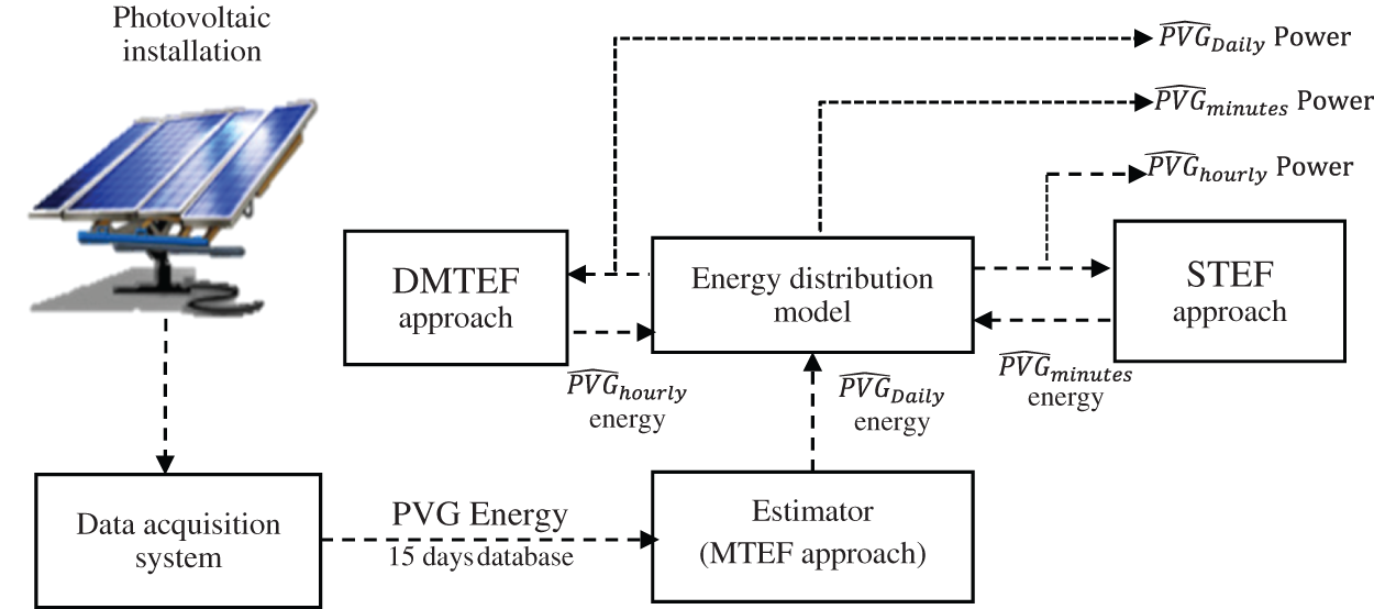
Figure 1: PVG forecast architecture

2.1 MTEF Approach

The MTEF approach consists of performing a dynamic estimation of PVG^Daily with respect to two steps:

Step 1: The PVG is forecasted for one day ahead based on the previous 15 days measurements of PVG energy.

Step 2: Gaussian distribution of the forecasted PVG to obtain an estimated PVG power curve from sunrise time to sunset time with 1 min time step.

The PVG^Daily is estimated for one day ahead based on time series measurements using the ARMA model [18–20]. The MTEF approach is composed of three major processes: the training process, the testing process and the forecasting process. The ARMA model is selected thanks to its simplicity and good forecasting accuracy. It is composed of two functions (Eq. (1)): the autoregressive (AR) function and the Moving Average (MA) function.

PVG^Day=∑h=1p⁡CARhPVG^Day−i+∑n=0q⁡CMAneDay−n (1)

where p and q are ARMA order parameters, CARh is the AR coefficient, CMAn the MA coefficient, eDay−n is the white noise.

The obtained PVG^Day is distributed by using a Gaussian distribution in order to estimate the PVG power (Eq. (2)).

PVG^(t)=πPVG^Day2(Daylight)Daysin(πt(Daylight)Day) (2)

where t is the time, PVG^Day the forecasted PVG of for one day ahead. (Daylight)Day is the forecasted daylight and obtained according to Eq. (3).

(Daylight)Day=tsunsetDay−tsunriseDay (3)

tsunriseDay is the sunrise time and tsunsetDay is the sunset time [21].

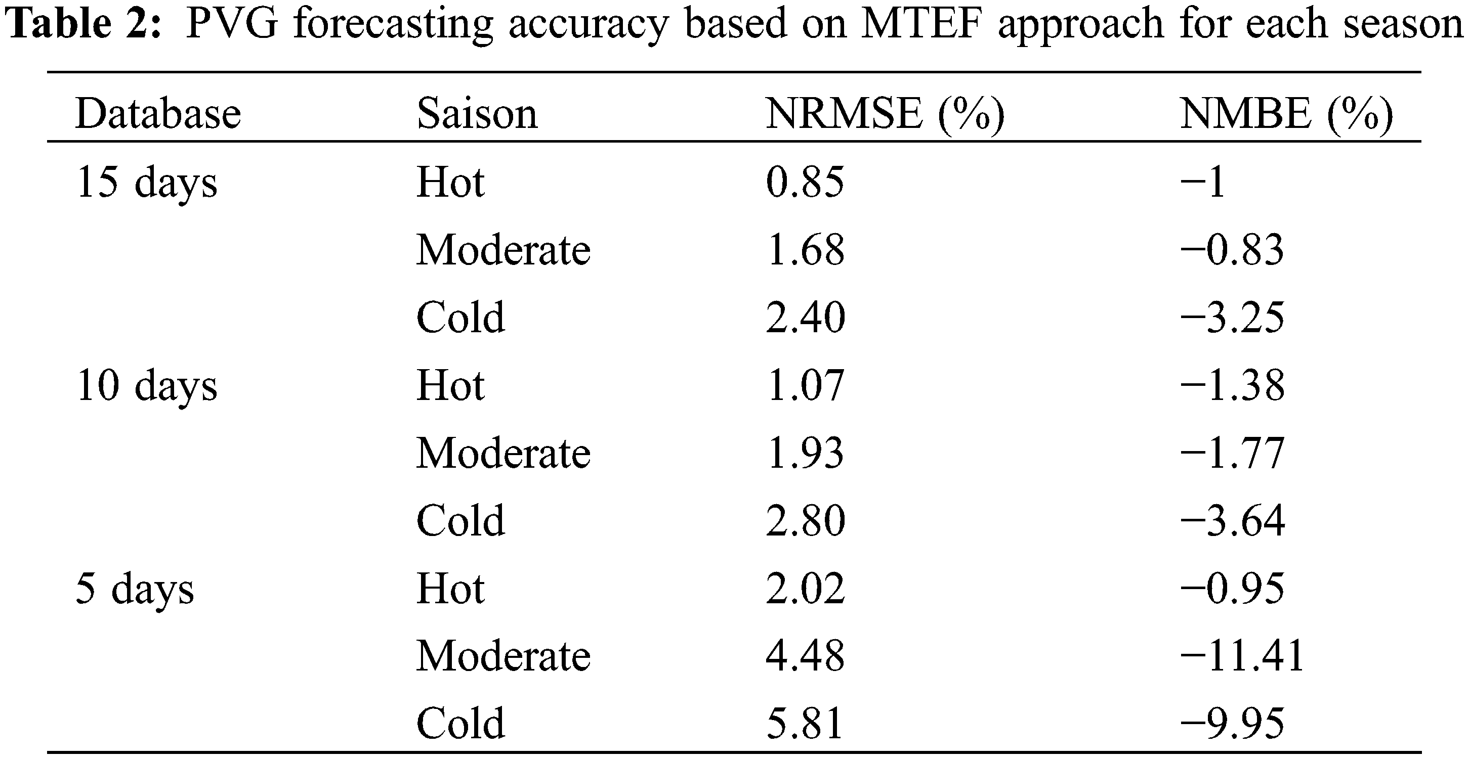
The time horizon selection is performed in order to test the forecasting accuracy of ARMA model by using the MTEF approach. The test is performed based on two kinds of data base. A data base of 365 days of the year 2019 and a seasonal data base organized into three seasons: a cold season (November, December, January and February), a moderate season (March, April, May and October), and a hot season (June, July, August and September). Furthermore, MTEF strategy is executed on three different time horizons (5 days, 10 days and 15 days) in order to select the best time horizon with the highest forecasting accuracy.

In order to evaluate the PVG forecasting accuracy, daily predicted and measured data were analyzed by computing the NRMSE and the NMBE errors for each prediction type:

NRMSE=1N∑i=1N⁡(estimatedvalue−measuredvalue)21N∑1N⁡masuredvalue×100 (4)

NMBE=∑i=1N⁡(estimatedvalue−measuredvalue)∑1N⁡measuredvalue×100 (5)

Tables 1 and 2 illustrate NRMSE and NMBE of PVG forecasting accuracy based on MTEF approach for the year 2019 and for each season, respectively.

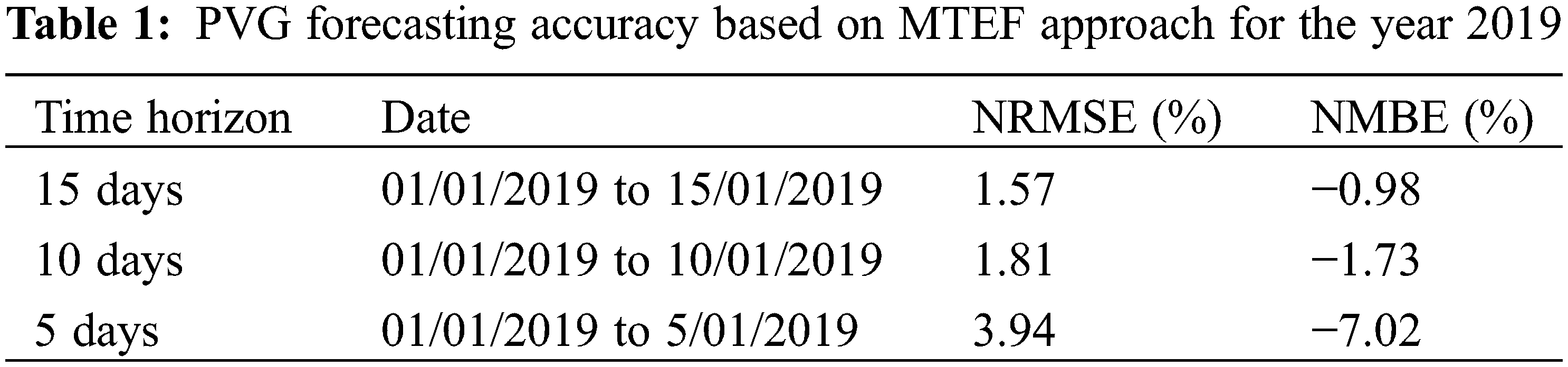
The MTEF reveals the best PVG forecasting accuracy using 15 days’ time horizon for the year 2019 data base with NRMSE = 1.57% and NMBE = −0.98%.

The MTEF reveals the best PVG forecasting accuracy over 15 days’ time horizon for the three seasons. The best season for the selected time horizon is the hot season with NRMSE = 0.85% and NMBE = −1%. The obtained results are explained by the high weather stability in the hot season compared to moderate and cold season.

2.2 DMTEF Approach

The DMTEF approach consists of performing the phenomenon of dynamicity by effectuating an hourly adjustment of the PVG^Daily curve of the 16th day obtained by the MTEF approach. The adjustment operation is mainly based on a relative error calculation between the hourly forecasted PVG energy ( PVG^hourly ) and the hourly measured PVG energy ( PVGhourly ) from sunrise time to sunset time. The adjustment decision is executed when the relative error is out of the interval between −5% and 5%. Such process increases the estimation accuracy of PVG^Daily . The following steps describe the DMTEF approach:

Step 1: The relative error calculation between the hourly forecasted PVG ( PVG^hourly ) and the hourly measured PVG ( PVGhourly ) is computed with respect to Eq. (6).

RE=PVGhourly−PVG^hourlyPVGhourly×100 (6)

Step 2: The adjustment decision is executed in case relative error (RE) is more than 5% or less than −5%. In such case, the estimated value is rejected and then replaced by the last measure PVG^hourly= PVGhourly .

2.3 STEF Approach

The STEF approach is a combination of PVG Short-Term (ST) forecasting and DMTEF approach. It consists of adjusting every 15 min the PVG^hourly obtained by the DMTEF approach considering the measured PVG in the previous two hours. Such process allows to increase the estimation accuracy of PVG^Daily for the rest of the day (from two hours after sunrise time to sunset time). The Auto-Regressive Integrated Moving Average (ARIMA) model is used to perform PVG Short-Term (ST) forecasting thanks to its approved use and good accuracy [22–28]. ARIMA is an extended part of the ARMA method known as AR integrated MA. The integrated part of ARIMA remove the non-stationary data. The following equations describe the ARIMA model:

αp(B)σdPVGt=βq(B)δ(t) (7)

αp(B)=1−θ1B−θ2B2−⋯−θPBP (8)

βq(B)=1−θ1B−θ2B2−⋯−θqBq (9)

where B is the backward shift operator, BPVGy=PVGy−1 , σ=1−B is the backward difference, the parameters αp and βq are the polynomials of orders p and q, respectively. The product of the AR part (p) described in Eq. (8), is an integrated part of I(d)=σ−1 , and the MA part (q) described in Eq. (9), composes the ARIMA (p, d, q) model. The following steps describe the STEF approach:

Step 1: The relative error calculation between the forecasted PVG every 15 min by STEF approach ( PVG^minutes,STEF ) and the measured PVG ( PVGminutes ) is computed with respect to Eq. (6).

RESTEF=PVGminutes−PVG^minutes,STEFPVGminutes×100 (10)

Step 2: Recalculate the relative error obtained in Eq. (6) by considering 15 min as time horizon between the forecasted PVG ( PVG^minutes,DMTEF ) and the measured PVG ( PVGminutes ) with respect to Eq. (11).

REDMTEF=PVGminutes−PVG^minutes,DMTEFPVGminutes×100 (11)

Step 3: The adjustment decision consists of attributing to PVG^minutes the value of PVGminutes,STEF or PVGminutes,DMTEF that presents the lowest relative error RESTEF and REDMTEF .

PVG^minutes= PVGminutes,STEF if RESTEF<REDMTEF

Otherwise, PVG^minutes= PVGminutes,DMTEF

3  Results and Discussion

The MTEF, DMTEF and STEF approaches are to be integrated into a management algorithm of a standalone PVG/Battery installation (Fig. 2). It is fundamentally composed of two power supply sources (a 3 KWp PVG and a battery bank of 273 Ah), a DC/AC inverter and two loads (a 350 W cold room and a one horsepower water pump) used in agricultural purpose. The aim is to make pragmatic decision on the times of supplying loads by considering the estimated PVG on the one hand and loads constraints and priorities on the second hand. In fact, the cold room must be continuously supplied as for the water pump, it must be switched on only if the battery is fully charged and for as long as possible depending on the estimated available energy. Other loads under different operation criteria and lower priorities may be added.

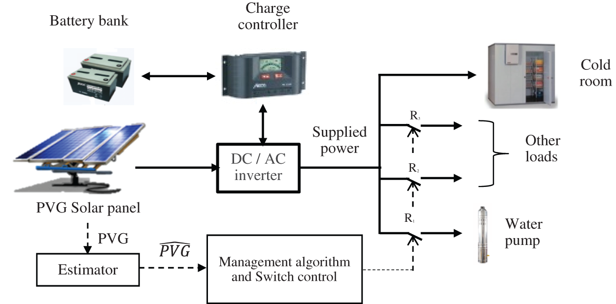
Figure 2: Off-grid PVG/Battery installation

3.1 MTEF Accuracy

In order to test the forecasting accuracy of ARMA model based on MTEF approach, a data base of 15 days for a stable and perturbed period is adopted considering the obtained results of time horizon selection presented in Section 3.1.

Figs. 3 and 4 show simulation results of MTEF approach based on ARMA model for the two selected periods, respectively.

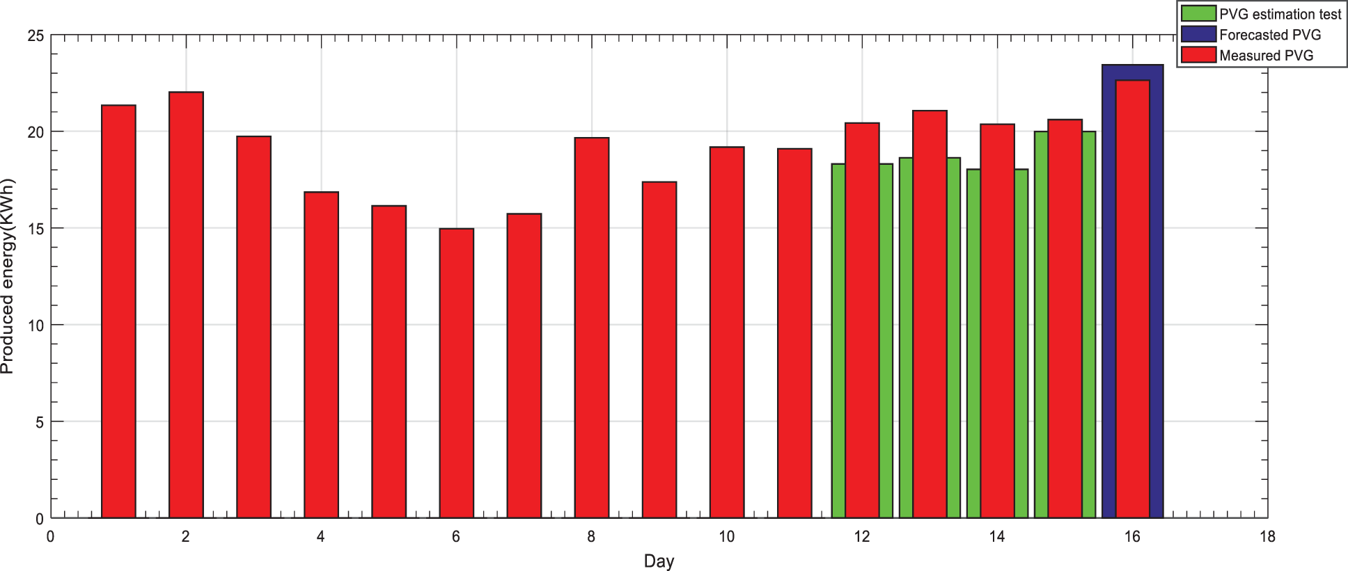
Figure 3: MTEF approach based on ARMA model for a stable period

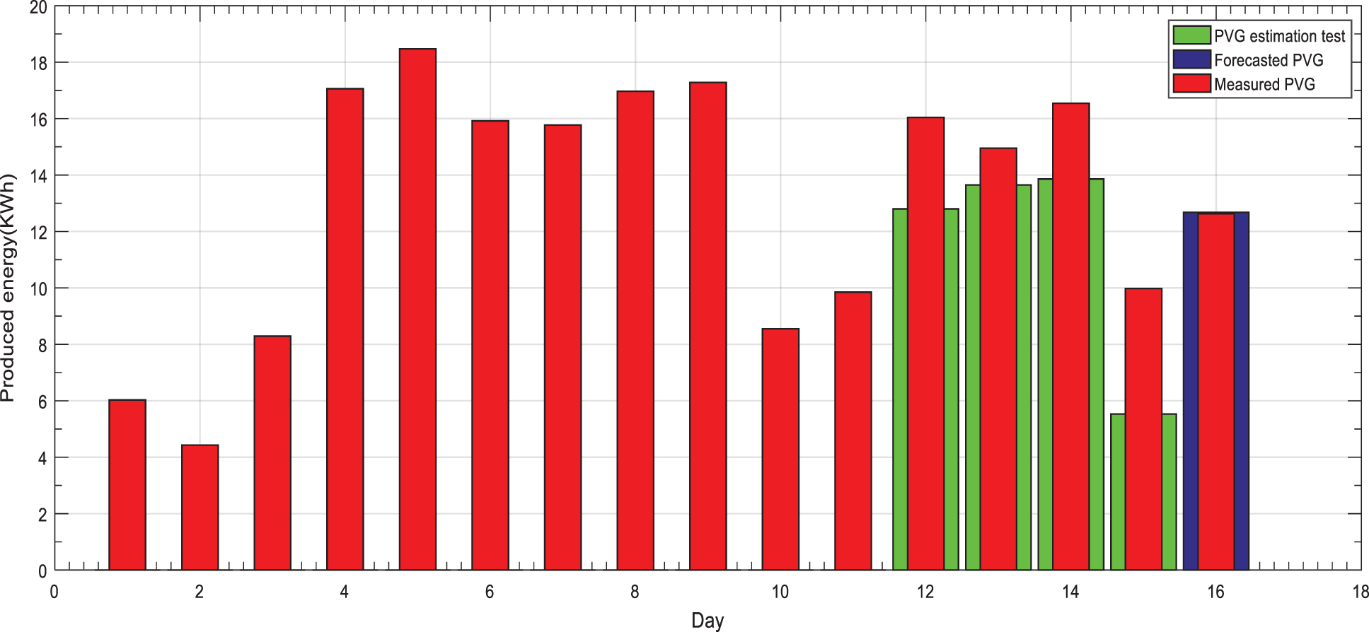
Figure 4: MTEF approach based on ARMA model for a perturbed period

Both figures reveal a good forecasting accuracy results of MTEF approach based on ARMA model in both periods.

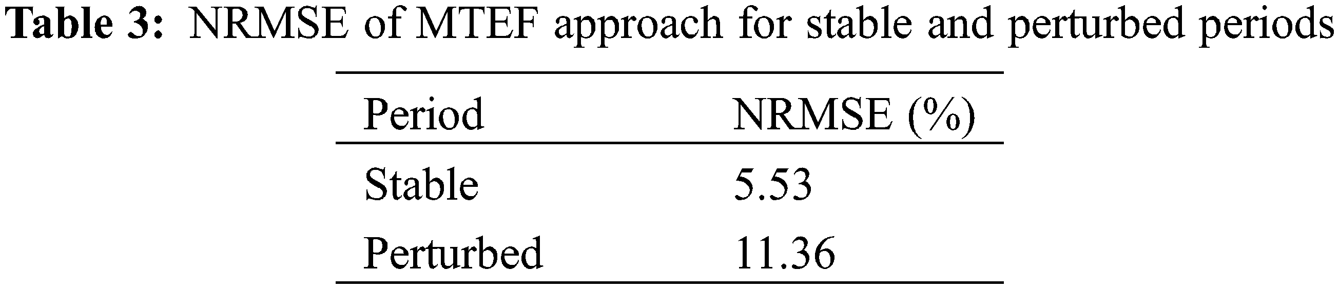
Table 3 illustrates the NRMSE of the stable and perturbed periods:

Figs. 5 and 6 show simulation results of the distribution of the forecasted PVG^Daily by MTEF approach based on ARMA model for the two selected periods, respectively.

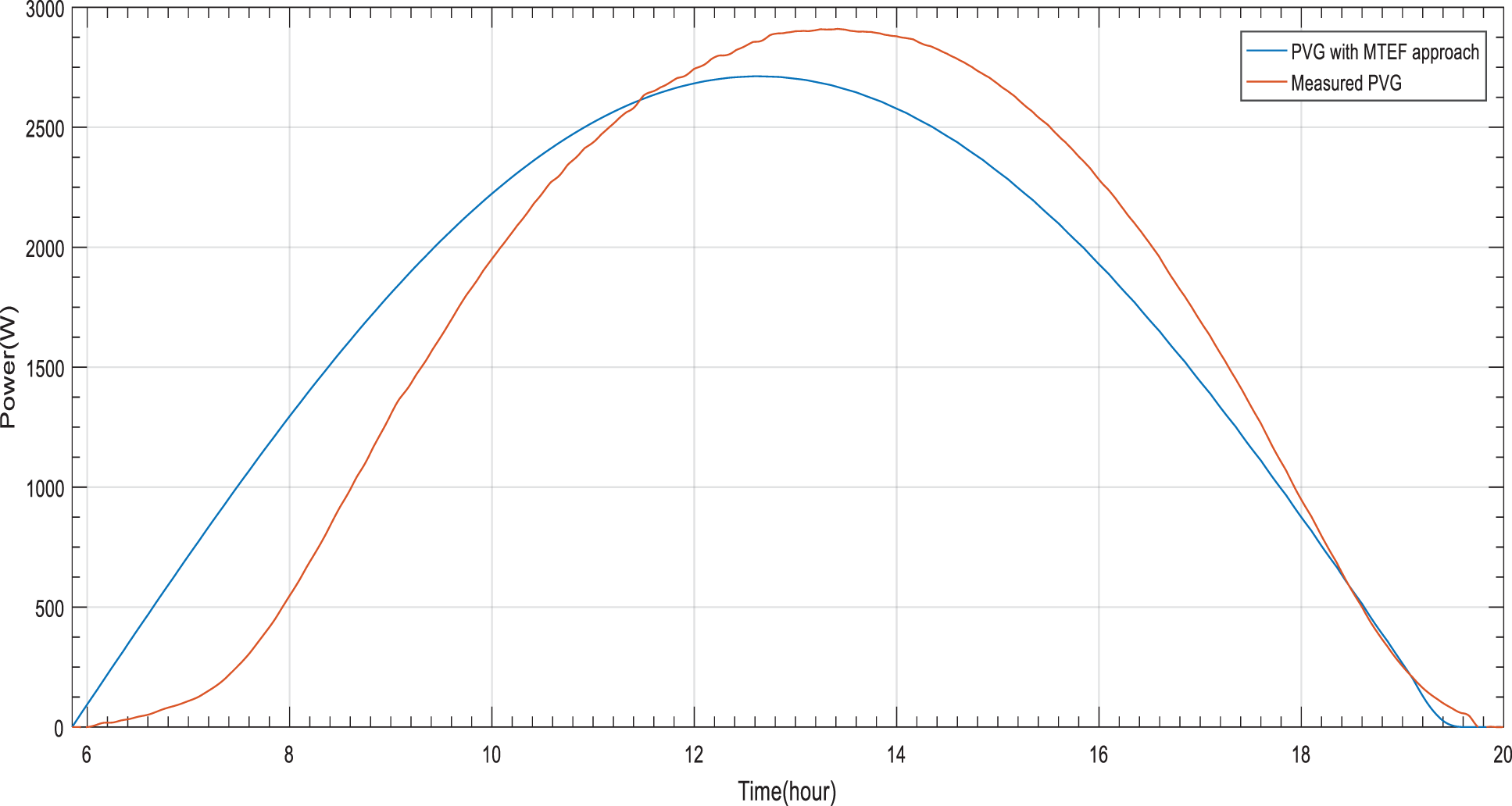
Figure 5: PVG estimation based on MTEF approach for a stable day

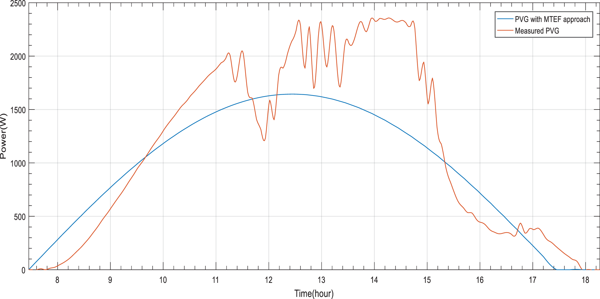
Figure 6: PVG estimation based on MTEF approach for a perturbed day

Both figures show good results but not optimal. From sunrise to sunset, a significant dissimilarity is noticed between the distribution of the forecasted PVG^Daily by MTEF approach based on ARMA model and measurements for the considered periods (Figs. 5 and 6). As for stable period, the measured PVG energy is 22.74 KWh and the forecasted PVG energy by MTEF approach is 23.43 KWh. As for perturbed period, the measured PVG energy is 12.33 KWh and the forecasted PVG energy by MTEF approach is 10.45 KWh. The acquired excess or loss of forecasted PVG energy may influence load’s operation of the standalone PVG/Battery installation system under study. PVG estimation may become more accurate with DMTEF approach and STEF approach.

Table 4 illustrates the NMBE of the stable and perturbed days:

3.2 DMTEF Accuracy

The DMTEF approach is used to perform dynamicity on the MTEF approach by effectuating an adjustment every hour of the estimated PVG^Daily . The accuracy of the DMTEF approach is tested based on two typical days: a perturbed day (November 16) and a stable day (May 01). Figs. 7 and 8 show simulation results of DMTEF approach.

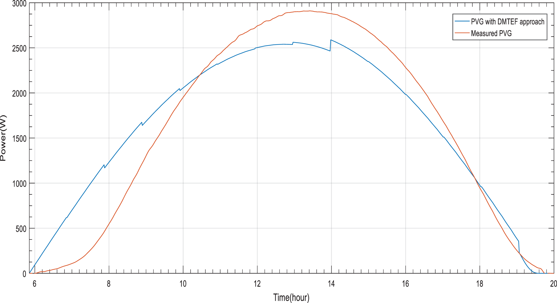
Figure 7: PVG estimation based on DMTEF approach for a stable day

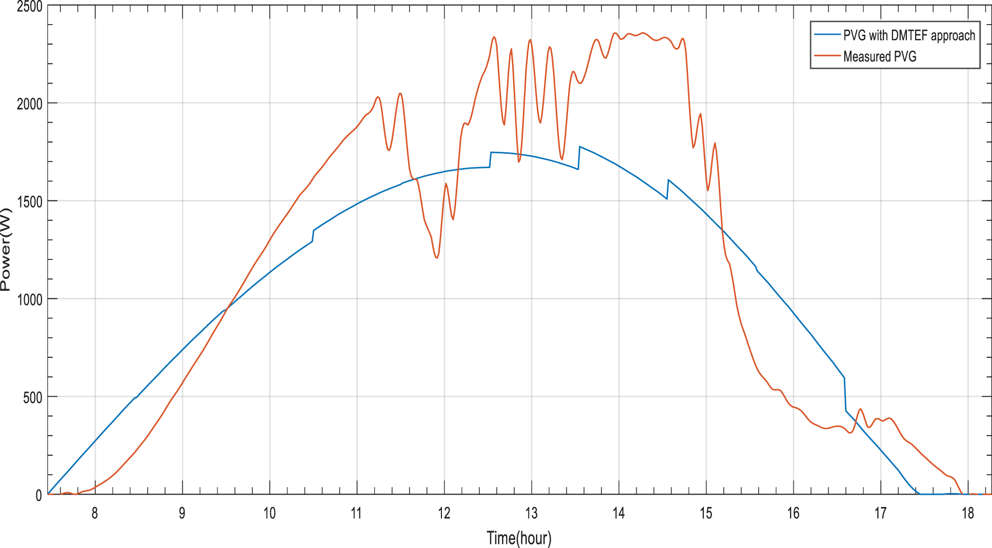
Figure 8: PVG estimation based on DMTEF approach for a perturbed day

The obtained results reveal an optimization of PVG estimation based on DMTEF. The proposed dynamicity offers a noticeable increasing of The PVG estimation accuracy between the distribution of the adjusted PVG^Daily by DMTEF approach and measurements for the considered periods (Figs. 7 and 8). As for stable period, the forecasted PVG energy by DMTEF approach is improved to become 22.88 KWh compared to the estimation given by MTEF approach. As for perturbed period, the forecasted PVG energy by DMTEF approach is improved to become 11.22 KWh. The acquired excess or loss of forecasted PVG energy is reduced compered to MTEF approach. Thus, the doubt about load operation is reduced.

Table 5 illustrates the NMBE of the stable and perturbed days:

3.3 STEF Accuracy

The STEF approach makes use of ST forecasting in order to forecast PVG every 15 min considering the previous measured 2 h based on the ARIMA model. Such approach performs an adjustment of the previous estimated PVG^Hourly by DMTEF approach every 15 min. Figs. 9 and 10 show simulation results of ST forecasting and Figs. 11 and 12 show simulation results of STEF approach.

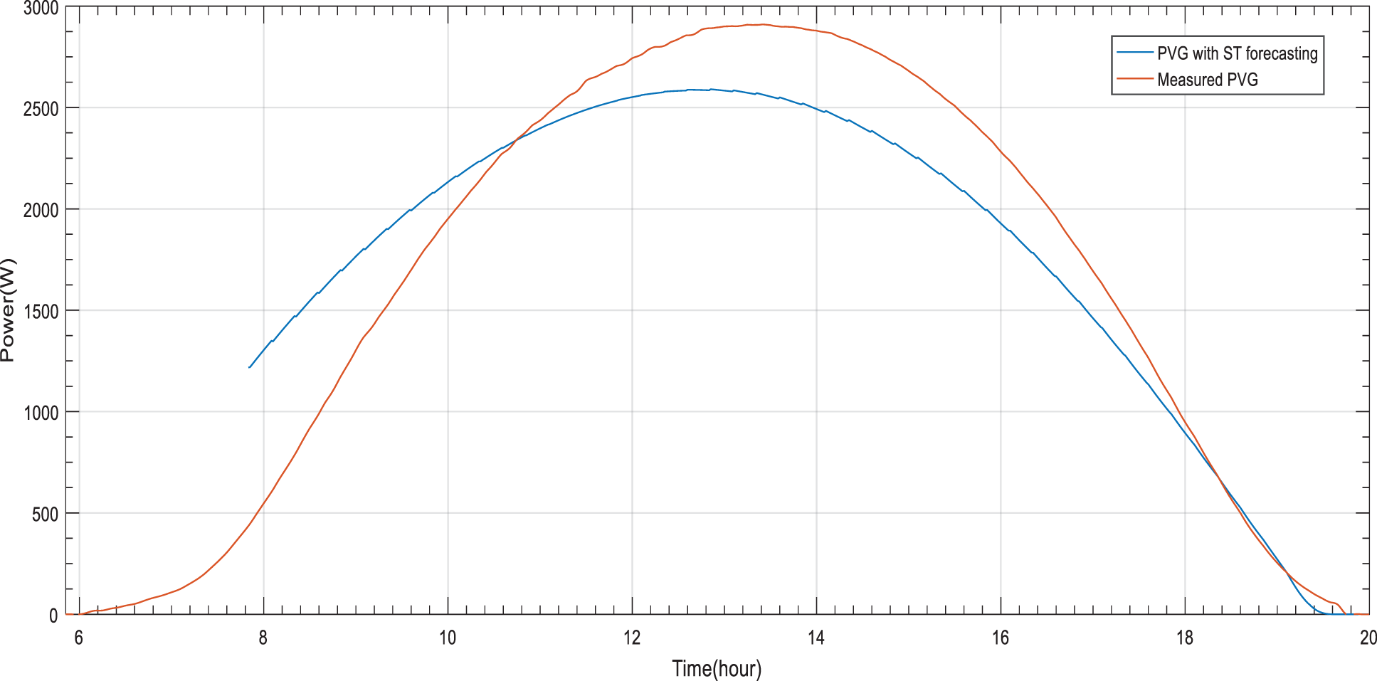
Figure 9: PVG estimation based on ST forecasting for a stable day

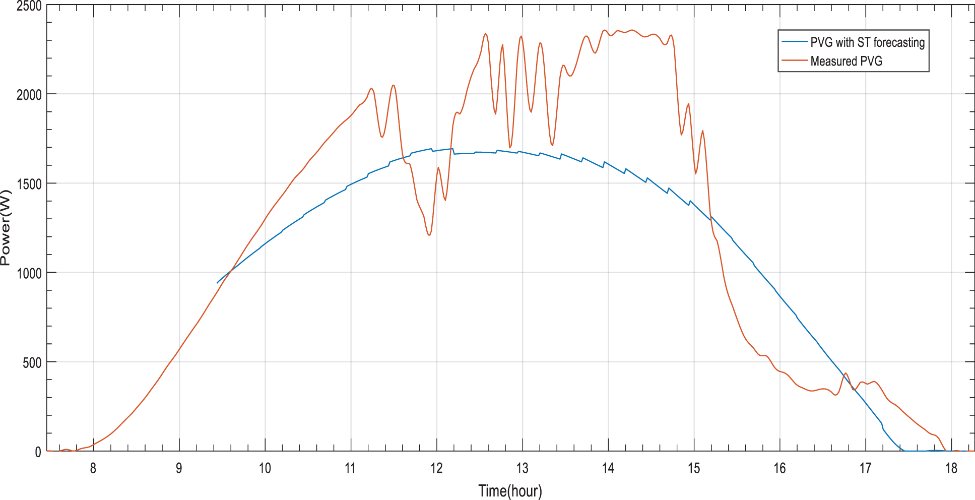
Figure 10: PVG estimation based on ST forecasting for a perturbed day

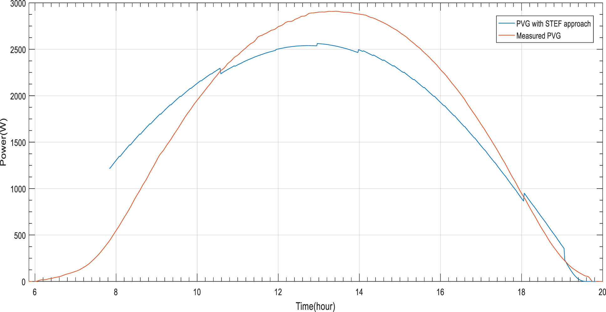
Figure 11: PVG estimation based on STEF approach for a stable day

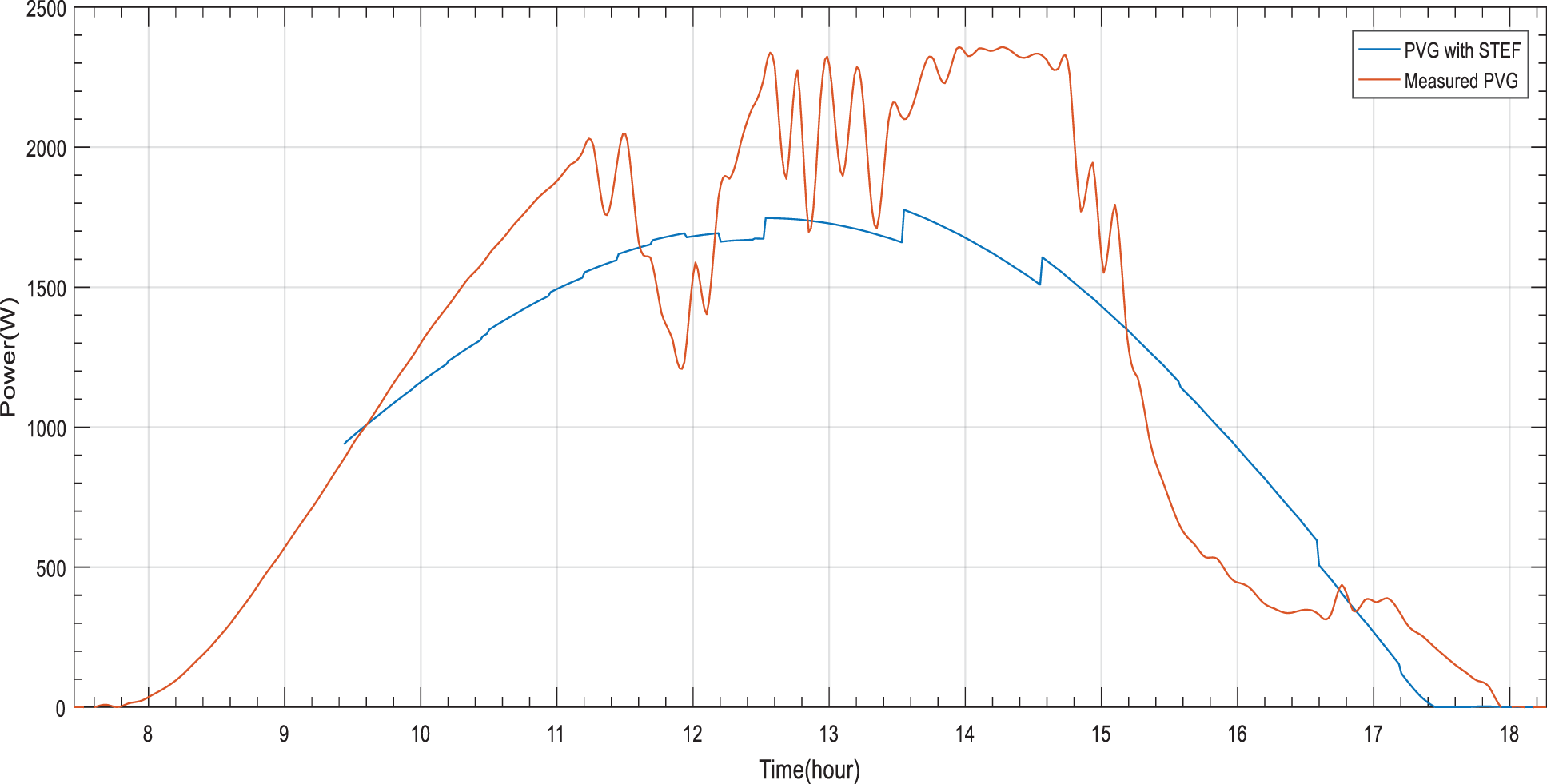
Figure 12: PVG estimation based on STEF approach for a perturbed day

The obtained results reveal an optimization of PVG estimation based on ST forecasting. Such approach offers a noticeable increasing of The PVG estimation accuracy between the distribution of the estimated PVG^Daily by ST forecasting and measurements for the considered periods (Figs. 9 and 10). As for stable period, the forecasted PVG energy by ST forecasting is improved to become 22.88 KWh compared to MTEF approach. As for perturbed period, the forecasted PVG energy by DMTEF approach is improved to become 11.08 KWh. The acquired excess or loss of forecasted PVG energy is reduced compered to MTEF approach. Thus, the risk about load not convenient operation times is reduced.

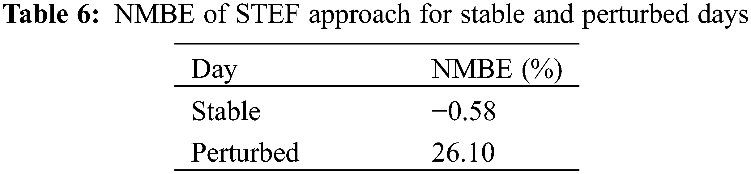
The obtained results reveal an optimization of PVG estimation based on STEF. An increasing of the PVG estimation accuracy is clearly noticed between the distribution of the adjusted PVG^Daily by STEF approach and measurements for the considered periods (Figs. 11 and 12). As for stable period, the forecasted PVG energy by STEF approach is improved to become 22.83 KWh compared to MTEF, DMTEF and ST approach. As for perturbed period, STEF approach keep dominance compared to the aforementioned approaches by improving the forecasted PVG energy to become 11.34 KWh. Such optimization offers more reliable and convenient load operation management.

Table 6 illustrates the NMBE of the stable and perturbed days:

3.4 Simulation Results of Sources and Loads Operation of PVG/Battery Installation Based on MTEF, DMTEF and STEF Approaches

The standalone PVG/Battery installation system is used to test the impact of the accuracy of the proposed STEF approach on the loads operation in compared to what it was previously with MTEF approach. The battery bank is used as a precaution source in anticipation of worst cases (lack of load supply by PVG source observed after performing STEF approach). As for loads, the major adjustment will appear in the water pump profile considering the continuous supply of the cold room. Figs. 13 and 14 show simulation results of sources and loads operation of PVG/Battery installation based on MTEF and STEF approaches.

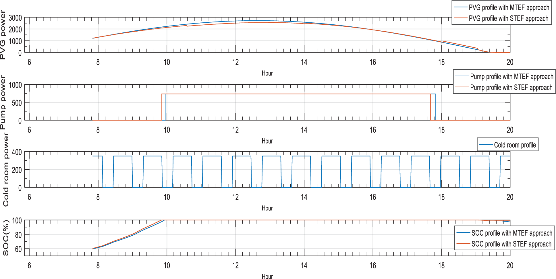
Figure 13: sources and loads profile with MTEF and STEF approaches in stable day

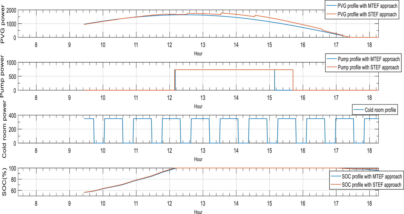
Figure 14: Sources and loads profile with MTEF and STEF approaches in perturbed day

The obtained results of Figs. 12 and 13 show a clear variation of the water pump operation duration in stable and perturbed day. The optimization of PVG forecasting accuracy obtained by STEF approach offer more reliable and convenient load operation to the PVG/Battery installation system under study. The battery SOC keep a balanced profile and has no intervention thanks to the PVG source capability to supply loads from sunset to sunrise.

4  Conclusion

A dynamic forecasting of Photovoltaic Energy Generation (PVG) was developed and experimentally tested in a management system of a standalone PVG/Battery installation. The methodology consists of forecasting PVG for three time period ahead: daily, hourly and for each 15 min. First, the MTEF approach forecasts the PVG using an ARMA model for a day ahead based on 15 days data base of measures. Then the DMTEF approach adjusts the hourly obtained PVG by MTEF approach considering the relative error. Finally, a STEF approach combines DMTEF approach and PVG Short-Term (ST) forecasting, based on ARIMA model, to adjust estimated PVG every 15 min. Obtained results show good concordance between the three kinds of forecast with measures. Besides, the load operation is improved and the battery safety is respected in stable and perturbed days. Future works aims to improve the accuracy of the proposed strategy in more than one day (stable and perturbed) and with different PVG installations (Grid connected and hybrid PVG systems).

Acknowledgement: This work has been developed thanks to the support of SIME Laboratory, Tunisia and the Department of Electric, Electronic and Computer Engineering, University of Catania, Italy.

Funding Statement: The authors received no specific funding for this study.

Conflicts of Interest: The authors declare that they have no conflicts of interest to report regarding the present study.

References

 1.  Antonanzas, J., Osorio, N., Escobar, R., Urraca, R., Martinez-de-Pison, F. J. et al. (2016). Review of photovoltaic power forecasting. Solar Energy, 136(10), 78–111. DOI 10.1016/j.solener.2016.06.069. [Google Scholar] [CrossRef]

 2.  Akhter, M. N., Mekhilef, S., Mokhlis, H., Shah, N. M. (2019). Review on forecasting of photovoltaic power generation based on machine learning and metaheuristic techniques. IET Renewable Power Generation, 13(7), 1009–1023. DOI 10.1049/iet-rpg.2018.5649. [Google Scholar] [CrossRef]

 3.  Das, U. K., Tey, K. S., Seyedmahmoudian, M., Mekhilef, S., Idris, M. Y. I. et al. (2018). Forecasting of photovoltaic power generation and model optimization: A review. Renewable Sustainable Energy Reviews, 81, 912–928. DOI 10.1016/j.rser.2017.08.017. [Google Scholar] [CrossRef]

 4.  Box, G. E., Jenkins, G. M., Reinsel, G. C., Ljung, G. M. (2015). Time series analysis: Forecasting and control. John Wiley & Sons. DOI 10.1111/jtsa.12194. [Google Scholar] [CrossRef]

 5.  Maria Grazia, D. G., Paolo Maria, C., Maria, M. (2014). Photovoltaic power forecasting using statistical methods: Impact of weather data. IET Science Measurement & Technology, 8(3), 90–97. DOI 10.1049/iet-smt.2013.0135. [Google Scholar] [CrossRef]

 6.  Jang, H. S., Bae, K. Y., Park, H. S., Sung, D. K. (2016). Solar power prediction based on satellite images and support vector machine. IEEE Transactions on Sustainable Energy, 7(3), 1255–1263. DOI 10.1109/TSTE.2016.2535466. [Google Scholar] [CrossRef]

 7.  Rosiek, S., Alonso-Montesinos, J., Batlles, F. J. (2018). Online 3-H forecasting of the power output from a BIPV system using satellite observations and ANN. International Journal of Electrical Power, 99(11), 261–272. DOI 10.1016/j.ijepes.2018.01.025. [Google Scholar] [CrossRef]

 8.  Aguiar, L. M., Pereira, B., Lauret, P., Diaz, F., David, M. (2016). Combining solar irradiance measurements, satellite-derived data and a numerical weather prediction model to improve intra-day solar forecasting. Renewable Energy, 97(4), 599–610. DOI 10.1016/j.renene.2016.06.018. [Google Scholar] [CrossRef]

 9.  Bright, J. M., Killinger, S., Lingfors, D., Engerer, N. A. (2018). Improved satellite-derived PV power nowcasting using real-time power data from reference PV systems. Solar Energy, 168, 118–139. DOI 10.1016/j.solener.2017.10.091. [Google Scholar] [CrossRef]

10. Barbieri, F., Rajakaruna, S., Ghosh, A. (2017). Very short-term photovoltaic power forecasting with cloud modeling: A review. Renewable Sustainable Energy Reviews, 75(1), 242–263. DOI 10.1016/j.rser.2016.10.068. [Google Scholar] [CrossRef]

11. Huang, Y., Lu, J., Liu, C., Xu, X., Wang, W. et al. (2010). Comparative study of power forecasting methods for PV stations. International Conference on Power System Technology, pp. 1–6. Hangzhou: IEEE. [Google Scholar]

12. Alfredo, N., Emanuele, O., Sonia, L., Alessandro, M. P., Adel, M. et al. (2019). Day-ahead photovoltaic forecasting: A comparison of the most effective techniques. Energies, 12(9), 1621. DOI 10.3390/en12091621. [Google Scholar] [CrossRef]

13. Voyant, C., Paoli, C., Muselli, M., Nivet, M. L. (2013). Multi-horizon solar radiation forecasting for Mediterranean locations using time series models. Renewable Subtainable Energy, 28(2), 44–52. DOI 10.1016/j.rser.2013.07.058. [Google Scholar] [CrossRef]

14. Zaharim, A., Razali, A., Gim, T. P., Sopian, K. (2009). Time series analysis of solar radiation data in the tropics. European Journal of Scientific Research, 25, 672–678. [Google Scholar]

15. Boland, J. (2008). Time series and statistical modelling of solar radiation, recent advances in solar radiation modelling. pp. 283. Springer Verlag. DOI 10.1007/978-3-540-77455-6_11. [Google Scholar] [CrossRef]

16. David, M., Ramahatana, F., Trombe, P. J., Lauret, P. (2016). Probabilistic forecasting of the solar irradiance with recursive ARMA and GARCH models. Solar Energy, 133, 55–72. DOI 10.1016/j.solener.2016.03.064. [Google Scholar] [CrossRef]

17. Benard, C., Boileau, E., Guerrier, B. (1985). Modeling of global solar irradiation using ARMA processes: Application to low-time (hourly) prediction, with a view to establishing optimal control in the habitat. Revue Physique, 20, 845. [Google Scholar]

18. Sansa, I., Boussaada, Z., Bellaaj, N. M. (2021). Solar radiation prediction using a novel hybrid model of ARMA and NARX. Energies, 14(21), 6920. DOI 10.3390/en14216920. [Google Scholar] [CrossRef]

19. Souissi A., Guidara I., Chaabene M. (2020). Dynamic forecasting-based load control of an autonomous photovoltaic installation. Computers and Electrical Engineering, 85(5), 106674. DOI 10.1016/j.compeleceng.2020.106674. [Google Scholar] [CrossRef]

20. Colak, I., Yesilbudak M., Genc, N., Bayindir, R. (2015). Multi-period prediction of Solar Radiation using ARMA and ARIMA Models. 2015 IEEE 14th International Conference on Machine Learning and Applications (ICMLA), pp. 1045–1049. [Google Scholar]

21. Chaabene, M. (2008). Measurements based dynamic climate observer. Solar Energy, 82, 9(9), 763–771. DOI 10.1016/j.solener.2008.03.003. [Google Scholar] [CrossRef]

22. Huang, R., Huang, T., Gadh, R., Li, N. (2012). Solar generation prediction using the ARMA model in a laboratory level micro-grid. IEEE Proceedings of the Third International Conference on Smart Grid Communications (Smart Grid Comm), pp. 528–533. IEEE. DOI 10.1109/SmartGridComm.2012.6486039. [Google Scholar] [CrossRef]

23. Gordon, R. (2009). Predicting solar radiation at high resolutions: A comparison of time series forecasts. Solar Energy, 83(3), 342–349. DOI 10.1016/j.solener.2008.08.007. [Google Scholar] [CrossRef]

24. Yadav, A. K., Chandel, S. S. (2014). Solar radiation prediction using artificial neural network techniques: A review. Renewable Sustainable Energy, 33(3), 772–781. DOI 10.1016/j.rser.2013.08.055. [Google Scholar] [CrossRef]

25. Valipour, M., Banihabib, M. E., Behbahani, S. M. R. (2013). Comparison of the ARMA, ARIMA, and the autoregressive artificial neural network models in forecasting the monthly inflow of Dez dam reservoir. Journal of Hydrologie, 476(10), 433–441. DOI 10.1016/j.jhydrol.2012.11.017. [Google Scholar] [CrossRef]

26. Belmahdi, B., Louzazni, M., Bouardi, A. E. (2020). One month-ahead forecasting of mean daily global solar radiation using time series models. Optik, 165207. DOI 10.1016/j.ijleo.2020.165207. [Google Scholar] [CrossRef]

27. Pieri, E., Kyprianou, A., Phinikarides, A., Makrides, G., Georghiou, G. E. (2017). Forecasting degradation rates of different photovoltaic systems using robust principal component analysis and ARIMA. IET Renewable Power Generation, 11(10), 1245–1252. DOI 10.1049/iet-rpg.2017.0090. [Google Scholar] [CrossRef]

28. Mbaye, A., Ndiaye, M., Ndione, D., Diaw, M., Traoré, V. et al. (2019). ARMA model for short-term forecasting of solar potential: Application to a horizontal surface on Dakar site. Materials and Devices, 4(1). DOI 10.23647/ca.md20191103. [Google Scholar] [CrossRef]

This work is licensed under a Creative Commons Attribution 4.0 International License, which permits unrestricted use, distribution, and reproduction in any medium, provided the original work is properly cited.