| Fluid Dynamics & Materials Processing |
DOI: 10.32604/fdmp.2022.022060
ARTICLE
Optimal Experiment Design for the Identification of the Interfacial Heat Transfer Coefficient in Sand Casting
University of Monastir, National Engineering School of Monastir, Laboratory of Thermal and Energy Systems Studies (LESTE), Monastir, LR99ES31, Tunisia
*Corresponding Author: Dorsaf Khalifa. Email: khalifadorsaf8@gmail.com
Received: 18 February 2022; Accepted: 25 March 2022
Abstract: The interfacial heat transfer coefficient (IHTC) is one of the main input parameters required by casting simulation software. It plays an important role in the accurate modeling of the solidification process. However, its value is not easily identifiable by means of experimental methods requiring temperature measurements during the solidification process itself. For these reasons, an optimal experiment design was performed in this study to determine the optimal position for the temperature measurement and the optimal thickness of the rectangular cast iron part. This parameter was identified using an inverse technique. In particular, two different algorithms were used: Levenberg Marquard (LM) and Monte Carlo (MC). A numerical model of the solidification process was associated with the optimization algorithm. The temperature was measured at different positions from the mould/metal interface at d = 0 mm (mould/metal interface), 30 mm, 60 mm and 90 mm. the thicknesses of the cast part were: L1 = 40 mm, 60 mm and 80 mm. A comparative study on the IHTC identification was then carried out by varying the initial value of the IHTC between 500 Wm−2K−1 and 1050 Wm−2K−1. Results showed that the MC algorithm used for estimating the IHTC gives the best results, and the optimal position was at d = 30 mm, the position closest to the mould/metal interface, for the lowest thickness L1 = 40 mm.
Keywords: Monte Carlo; interfacial heat transfer coefficient; Levenberg Marquard; optimal experiment design; sand casting
Nomenclature
| | Distance between the mould/metal interface and measuring point [mm] |
| | Initial defect vector |
| | Current defect vector |
| | Calculated error |
| | Solid fraction |
| | Identified value of the IHTC [Wm-2K-1] |
| | Initial value of the IHTC [Wm-2K-1] |
| | Exact value of the IHTC [Wm-2K-1] |
| | Iteration number |
| | Jacobian matrix |
| | Thermal conductivity [Wm-1K-1] |
| | Latent heat [kJ K-1] |
| | Casting thickness [mm] |
| | Number of the measurement evaluations |
| | Temperature [K] |
| | Ambient temperature [K] |
| | Computation time [s] |
| V | Objective function [K] |
| | Weight function |
| | Sensitivity vector |
| | Sensitivity coefficient at parameter |
| | Experimental measurement vector |
| | Ratio between the initial value and exact value of the IHTC |
| | Control parameter |
| | Volumetric heat capacity of the mould [Jm-3K-1] |
| | Normal derivative |
| | Identity matrix |
| | Specified optimally tolerance |
| | Defect reduction tolerance factor |
| | Control variable tolerance factor |
| Subscripts | |
| M | Mould |
| C | Cast-metal |
| Abbreviations | |
| IHTC | interfacial heat transfer coefficient |
| LM | Levenberg Marquard |
| LS | Least-squares |
| MC | Monte Carlo |
Casting simulation has become an indispensable tool to visualize mould solidification and cooling and predict defects [1,2]. However, the boundary conditions must be correctly defined, in particular, the thermal contact between the mould and the metal during these processes. In fact, determining the IHTC is a fundamental step in creating a reliable numerical model that can predict certain casting defects. Although the IHTC is very important, its value is not easily obtained using the direct experimental or theoretical method as it is influenced by various factors, such as alloy type, latent heat, thermo-physical properties of mould, initial mould temperature [3,4].
The inverse method is a very flexible methodology that can be applied to several processes, in particular, sand casting [5–7]. It consists in minimizing the square difference between numerical and experimental temperature measurements. In recent years, several studies have focused on the identification of the IHTC using inverse methods. For example, Zhang et al. [8] have developed an inverse conduction model to determine the heat flux and the IHTC for cylindrical casting in the lost foam process. Palumbo et al. [9] have proposed an optimization procedure to determine the IHTC and the solid fraction of superduplex stainless steel together with an optimal value of the latent heat in the sand casting process. Rajaraman et al. [10] have estimated the IHTC and the mould surface temperature during the solidification of a rectangular aluminium alloy casting in the sand mould by two different methods: control volume and Beck’s approach. Wang et al. [11] have proposed a method that combines weighted least squares with a modified LM method to estimate heat transfer coefficients in continuous casting. Vaka et al. [12] have estimated the IHTC using an inverse method based on the salp swarm algorithm in the continuous casting process. Stieven et al. [13] have proposed and analysed two different models based on inverse problems for the identification of the IHTC in unidirectional permanent mould casting. Researchers still identify the IHTC based on inverse methods, which shows the great importance of this coefficient. All of these studies have focused on the different methods of identifying the IHTC without investigating the influence of the thickness of the moulded part and the distance between the mould/metal interface and the measuring thermocouple.
Using arbitrary thickness of the rectangular cast iron part and position of the temperature measurement leads to inaccurate IHTC. Therfore, the objective of this study is to determine the optimal temperature measurement position and the optimal thickness of the rectangular cast part and also the best algorithm for the identification of the IHTC. A numerical model was associated with two different identification algorithms: Levengberg Marquard and Monte Carlo in order to create an optimal experiment design for the identification of the IHTC during solidification of hypo-eutectic cast iron in a sand mould. The results obtained from these two algorithms were then evaluated and compared for two initial values of the IHTC.
Sand casting process consists of pouring liquid metal into a green sand mould. This process is obtained by a succession of phenomena. The metal and the mould are subjected to strong temperature variations. When the cooled cast iron solidifies, it releases latent heat that is absorbed by the mould.
Therefore, in our case, we treat the phenomenon of heat transfer with phase change [14] which is described by Eq. (1):
The above mathematical model describes the phase change from liquid to solid phase by variation of solid fraction, which is sensitive to temperature variation as a function of time, hence:
The heat transfer in the mould is described by the following equation:
The external surface of the mould presents a thermal continuity given by the boundary condition:
Additionally, on the contact surface between mould and casting, the continuity condition:
2.2 Methodology of the Numerical Simulation
COMSOL software was used to simulate the solidification of a cast iron in a green sand mould. The following procedures were adopted for the simulation:
• A rectangular parallelepiped-shaped piece was used with dimensions 40 × 400 × 550 mm3. This geometry presents symmetry in three dimensions. However, in this work, the analysis was made for the half symmetry in 2-D. The concerned section belongs to the (x, z) plane shown in Fig. 1, and has two different parts: (a) is the metal and (b) is the sand mould. These two parts are joined by a thermal contact. (C) is the positions of temperature measurements: d = 0 mm (mould/metal interface), 30 mm, 60 mm, 90 mm
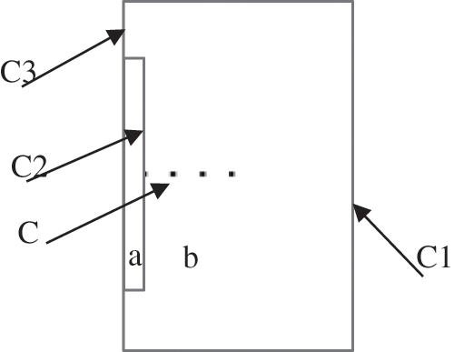
Figure 1: Numerical model
• The material used for the mould is green sand. Its properties are taken from the COMSOL database. The molten metal is grey cast iron and its properties are taken from previous work.
• The heat transfer in the casting is described by Eq. (1) and in the sand by Eq. (3). The initial conditions for the mould were the ambient temperature (300 K), and the temperature of metal taken as
The boundary conditions are:
C1: convective heat flux, described by Eq. (4),
C2: thermal contact, described by Eq. (5),
C3: symmetry
• The optimal mesh adopted in the simulation is the triangular type with a number of triangular elements equal to 678.
In this section, a sensitivity analysis was conducted to quantify the influence of variation of the IHTC on the temperature evolution at different positions in the sand mould. Sensitivity coefficients are calculated by the following expression:
where
In this section, a study of the identifiability of the IHTC at different positions in the sand mould is presented using two identification programs: LM and MC. Generally, parameter estimation is obtained by solving a least-squares (LS) optimization problem. In LS, we search for parameter values β that minimize the sum of squared differences between experimental and numerical measurements:
where
where µk is a scalar whose value varies from one iteration to another and Ω is the identity matrix.
The LM algorithm is based on the iterative expression:
On the other side, MC algorithm samples values (β) randomly with uniform distribution inside a box specified by the user.
Stopping criteria
For LM algorithm, we define:
Then, when the LM algorithm is used, the following conditions are used to determine when optimality has been reached:
• Terminate when the defect has been reduced enough; that is
• Terminate when the relative increment of the scaled control variable x is below the control variable tolerance; that is
• Terminate when the cosine between the defect and the Jacobian columns is below the optimality tolerance; that is
For the MC algorithm, the iteration stops when a new sampling point improves the objective function but is within the optimality tolerance to the previous best point.
The temperature measurements are simulated using two different values of the IHTC: 500 Wm-2K-1 and 1050 Wm-2K-1 [16]. These simulations were then used as numerical experiments to which the estimation process described above was applied. The identification is executed for different initial values, so we have defined a coefficient α representing the ratio between the initial value and exact value (h2) of the IHTC.
We, therefore, calculate the error between the exact value and the identified value by referring to the following equation:
Fig. 2 shows the evolution of sensitivity at various distances from the mould/metal interface.
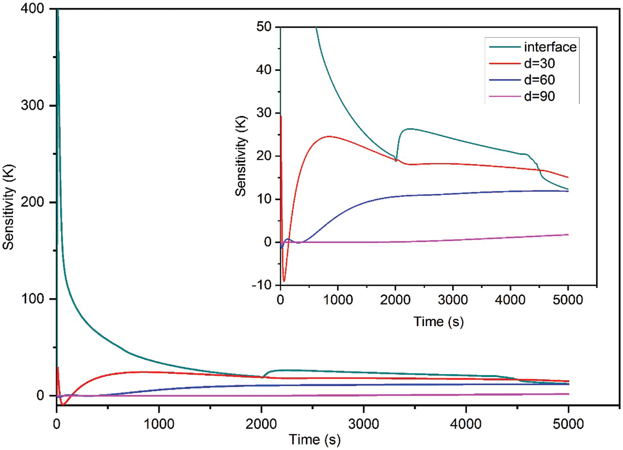
Figure 2: Sensitivities vs. time
The sensitivity coefficients for the IHTC in different positions attained the highest values at the interface (d = 0 mm) and close to the interface. As a result, it is difficult to estimate the IHTC at d = 90 mm which may not give an accurate estimation as the positions closer to the interface. It can be observed that the measurement position of the temperature far from the mould/metal interface is less sensitive. From the sensitivity analysis, the thermocouple should be placed near the unknown boundary condition (mould/metal interface) for a better estimation of unknown IHTC. Estimates were made using simulated temperatures to confirm the results of the sensitivity study. Table 1 shows the results of the sought coefficient h2 identification obtained for the exact input data. Specifically, the table contains the coefficient α, the relative errors, and the iterations number for the two optimization algorithms.
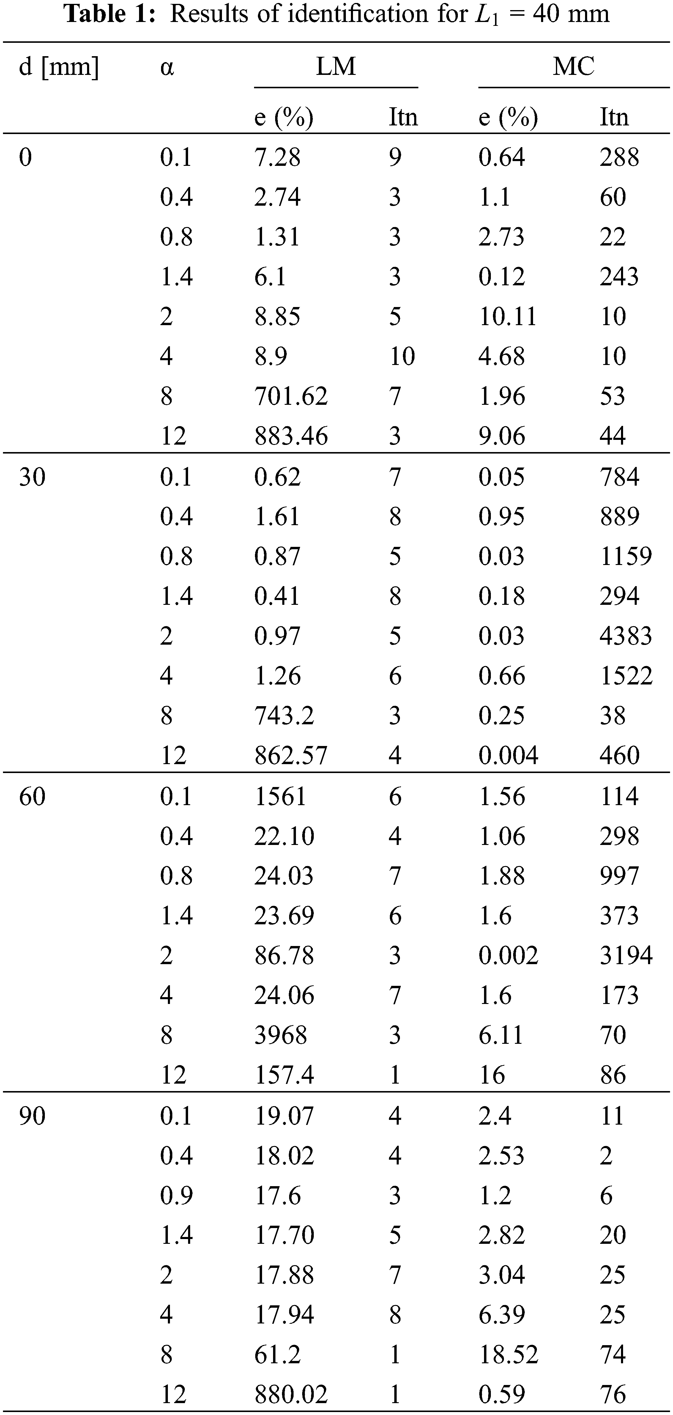
A comparison of the results obtained by the two algorithms showed that the relative error between the exact value and the identified value is smaller for the MC algorithm than that of the LM algorithm. For LM, the error varied between 0.41% and 1561% while for MC the error varied from 0.002% to 18.52%. We also notice that for initial values further than the exact value, for α = 12 and d = 30, the error was 0.004% for the MC algorithm while the LM algorithm showed a large error of 862.57%. In order to find the optimal position for the identification of the IHTC, we chose the MC algorithm. Fig. 3 represents the relative error for the MC algorithm at different distances from the metal-mould interface.
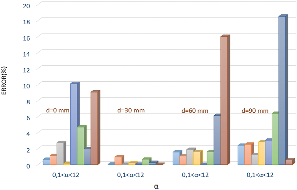
Figure 3: Relative errors for MC algorithm
It is clear that the best identification of the IHTC is at d = 30 mm, the position closest to the metal/mould interface, with a relative error of 0.004% to 0.95% for α between 0.1 and 12. This result indicates that large changes in the initial value of the estimated parameter do not influence the result of identification for MC algorithms. In the next section, the same approach was followed by varying the thickness L1 and the exact value of h2. Tables 2 and 3 show the relative errors obtained respectively for the initial value of h2 of 500 Wm-2K-1 and 1050 Wm-2K-1 and different thicknesses.

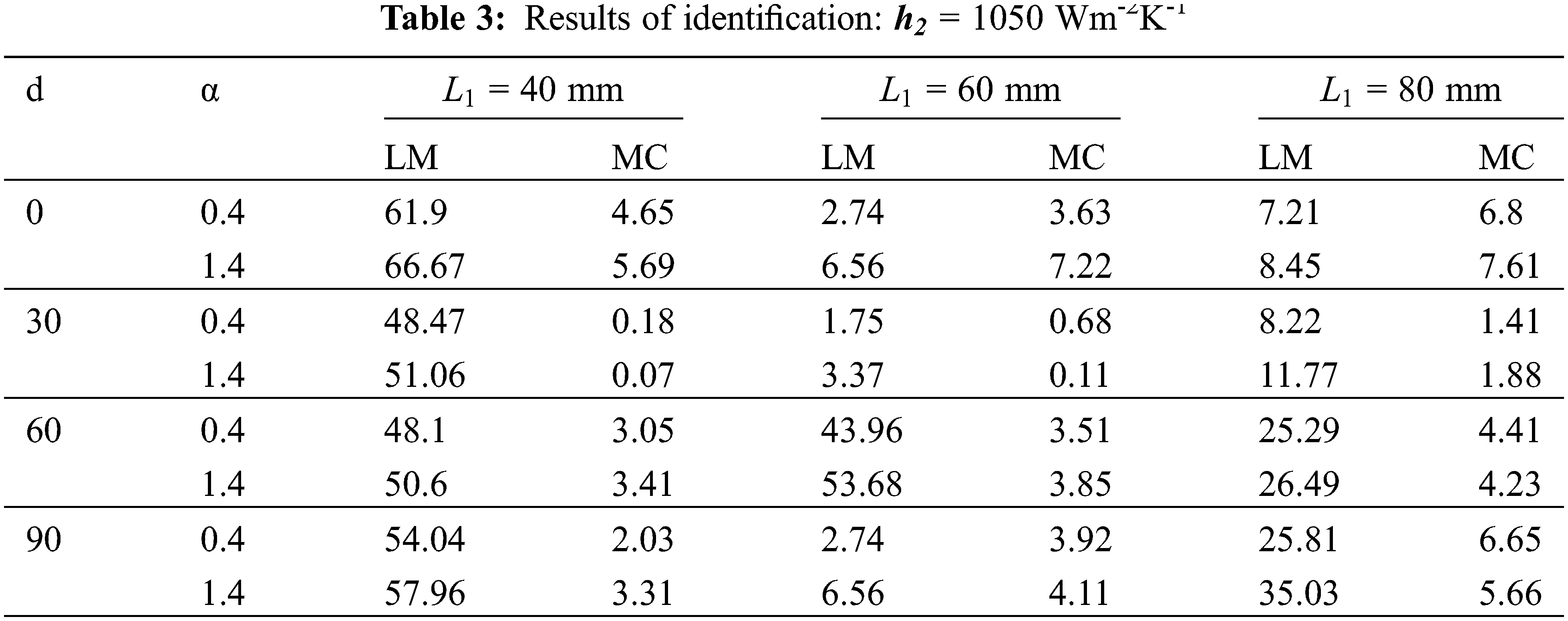
By analysing Tables 2 and 3, we note that the relative errors between the exact value and the identified value of the IHTC are smaller for the MC algorithm than the LM algorithm. In fact, for the MC algorithm, the error varies between 0.14% and 66.67%. However, for the MC algorithm the error varies from 0.07% to 22.47%. This may confirm that the MC algorithm used for estimating the IHTC gives the best results. Therefore, in order to find the optimal position and thickness, the identification procedure in the next part was carried out using the MC algorithm.
The optimal design of the experiment is summarized in Fig. 4. We can see that for different values of α, the calculated error is smaller for the lowest thickness (L1 = 40 mm). The best identification of the IHTC is at d = 30 mm with relative error of 0.95% for α = 0.4% and 0.18% for α = 1.4 for h2 = 500 Wm-2K-1. For h2 = 1050 Wm-2K-1, the error was equal to 0.18% for α = 0.4% and 0.07% for α = 1.4.
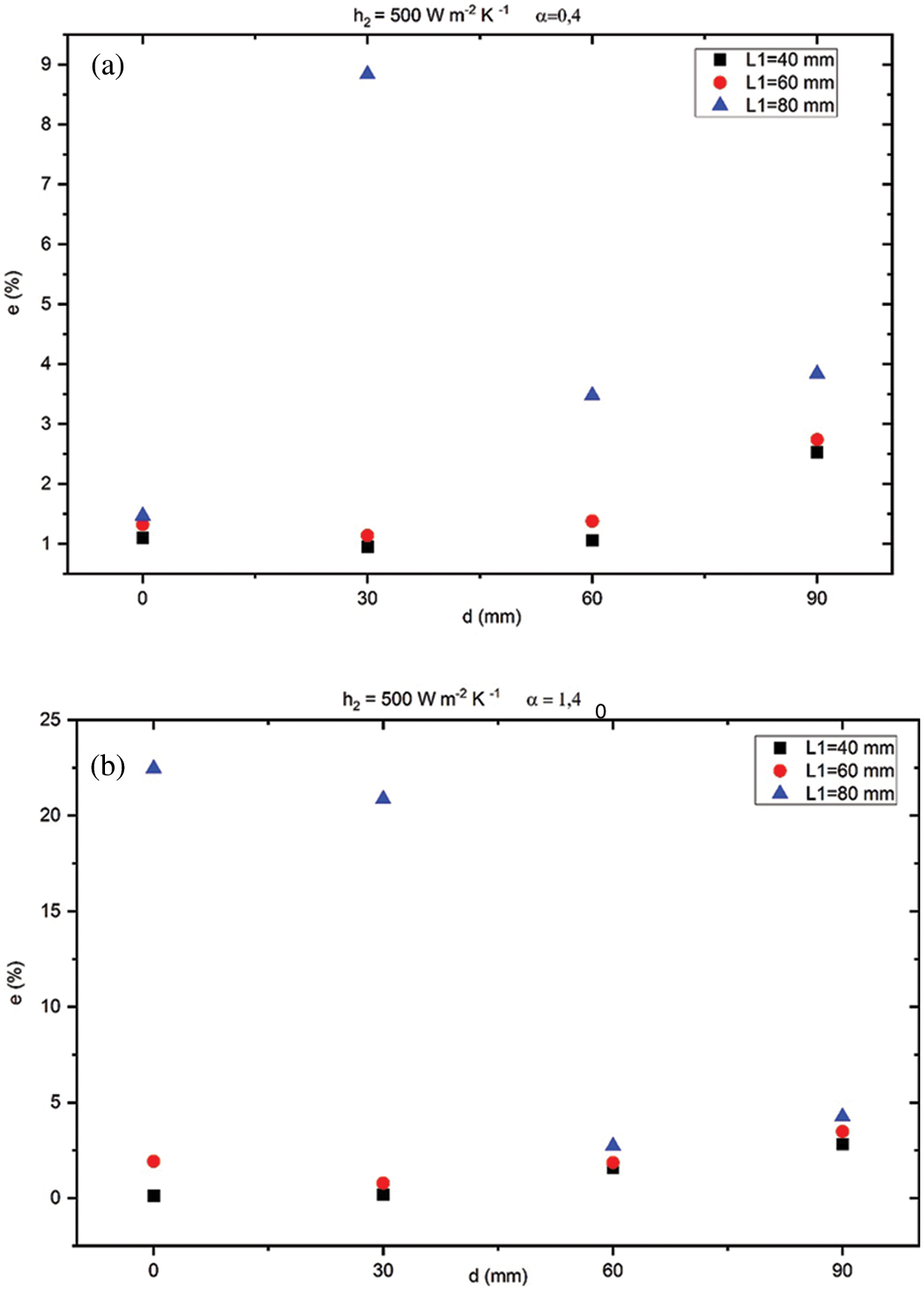

Figure 4: variation of the error of identification (a) α = 0.4 and h2 = 500 Wm-2K-1, (b) α = 1.4 and h2 = 500 Wm-2K-1, (c) α = 0.4 and h2 = 1050 Wm-2K-1, (d) α = 1.4 and h2 = 1050 Wm-2K-1
We can conclude that using MC algorithm, the optimal position for the identification of the IHTC is at d = 30 mm, the position closest to the mould/metal interface , for the lowest thickness
The scope of this study is an experiment design method using LM and MC algorithms to find the optimal position of temperature measurement and the optimal thickness of the rectangular cast iron part for the identification of the IHTC. Numerical simulations were calculated and considered as numerical experiments by measuring the temperature at different positions in sand during the solidification of a grey cast iron in a sand mould.
From the sensitivity study, the thermocouple should be placed near mould/metal interface for a better estimate of unknown IHTC.
The results of identification are divided into two parts:
A comparative study was carried out for the two algorithms LM and MC by varying the initial value of the IHTC and the distance d (d = 0 mm, 30 mm, 60 mm, 90 mm). The results showed that the relative error between the exact value and the identified value is smaller for the MC algorithm than for the LM algorithm. This indicates that large changes in the initial value of the estimated parameter do not influence the results of identification for MC algorithm.
On the other hand, the estimation was based on the MC algorithm by varying the initial value of the IHTC, the distance d and the thickness of the rectangular cast part
In order to complete this study, we aim to carry out experimental measurements of the temperature variation in a green sand mould and to identify the IHTC in the real condition of the casting process.
Acknowledgement: This project is carried out under the MOBIDOC Scheme, funded by the EU through the EMORI Program and managed by the ANPR.
Funding Statement: The authors received no specific funding for this study.
Conflicts of Interest: The authors declare that they have no conflicts of interest to report regarding the present study.
1. Dessai, P. P., Sohan, J., Vishal, L., Rajat, K., Prasad, G. et al. (2019). Use of casting simulation for yield improvement. International Research Journal of Engineering and Technology, 6(3), 7704–7707. [Google Scholar]
2. Vijayaram, T. R., Sulaiman, S., Hamouda, A. M. S., Ahmad, M. H. M. (2006). Numerical simulation of casting solidification in permanent metallic molds. Journal of Materials Processing Technology, 178(1–3), 29–33. DOI 10.1016/j.jmatprotec.2005.09.025. [Google Scholar] [CrossRef]
3. Hasan, H. S., Peet, M. J. (2012). Heat transfer coefficient and latent heat of martensite in a medium-carbon steel. International Communications in Heat and Mass Transfer, 39(10), 1519–1521. DOI 10.1016/j.icheatmasstransfer.2012.09.008. [Google Scholar] [CrossRef]
4. Wang, D., Zhou, C., Xu, G., Huaiyuan, A. (2014). Heat transfer behavior of top side-pouring twin-roll casting. Journal of Materials Processing Technology, 214(6), 1275–1284. DOI 10.1016/j.jmatprotec.2014.01.009. [Google Scholar] [CrossRef]
5. Chen, L., Wang, Y., Peng, L., Fu, P., Jiang, H. (2014). Study on the interfacial heat transfer coefficient between AZ91D magnesium alloy and silica sand. Experimental Thermal and Fluid Science, 54, 196–203. DOI 10.1016/j.expthermflusci.2013.12.010. [Google Scholar] [CrossRef]
6. Chang, T., Zou, C. M., Wang, H. W., Wei, Z. J., Zhang, X. J. (2020). Optimization of the interface heat transfer coefficient model based on the dynamic thermo-physical parameters in the pressure-temperature coupled field. International Communications in Heat and Mass Transfer, 110(18), 1–8. DOI 10.1016/j.icheatmasstransfer.2019.104435. [Google Scholar] [CrossRef]
7. Rajaraman, R., Velraj, R. (2008). Comparison of interfacial heat transfer coefficient estimated by two different techniques during solidification of cylindrical aluminum alloy casting. Heat and Mass Transfer, 44(9), 1025–1034. DOI 10.1007/s00231-007-0335-7. [Google Scholar] [CrossRef]
8. Zhang, L., Tan, W., Hu, H. (2016). Determination of the heat transfer coefficient at the metal–sand mold interface of lost foam casting process. Heat and Mass Transfer, 52(6), 1131–1138. DOI 10.1007/s00231-015-1632-1. [Google Scholar] [CrossRef]
9. Palumbo, G., Piglionico, V., Piccininni, A., Guglielmi, P., Sorgente, D. et al. (2015). Determination of interfacial heat transfer coefficients in a sand mould casting process using an optimised inverse analysis. Applied Thermal Engineering, 78, 682–694. DOI 10.1016/j.applthermaleng.2014.11.046. [Google Scholar] [CrossRef]
10. Rajaraman, L., Gowsalya, L. A., Velraj, R. (2018). Interfacial heat transfer coefficient estimation during solidification of rectangular aluminum alloy casting using two different inverse methods. Frontiers in Heat and Mass Transfer, 11, 1–8. DOI 10.5098/hmt.11.23. [Google Scholar] [CrossRef]
11. Wang, Y., Luo, X., Yu, Y., Yin, Q. (2016). Evaluation of heat transfer coefficients in continuous casting under large disturbance by weighted least squares Levenberg-Marquardt method. Applied Thermal Engineering, 111, 989–996. DOI 10.1016/j.applthermaleng.2016.09.154. [Google Scholar] [CrossRef]
12. Vaka, A. S., Ganguly, S., Talukdar, P. (2021). Novel inverse heat transfer methodology for estimation of unknown interfacial heat flux of a continuous casting mould: A complete three-dimensional thermal analysis of an industrial slab mould. International Journal of Thermal Sciences, 160, 1–13. DOI 10.1016/j.ijthermalsci.2020.106648. [Google Scholar] [CrossRef]
13. Stieven, G. D. M., Soares, D. D. R., Oliveira, E. P., Lins, E. F. (2021). Interfacial heat transfer coefficient in unidirectional permanent mold casting: Modeling and inverse estimation. International Journal of Heat and Mass Transfer, 166(11), 1–10. DOI 10.1016/j.ijheatmasstransfer.2020.120765. [Google Scholar] [CrossRef]
14. Mochnacki, B. (2011). Numerical modeling of solidification process. Computational Simulations and Application, 24, 513–542. DOI 10.5772/921. [Google Scholar] [CrossRef]
15. Pariona, M. M., Mossi, A. C. (2005). Numerical simulation of heat transfer during the solidification of pure iron in sand and mullite molds. Journal of the Brazilian Society of Mechanical Sciences and Engineering, 27(4), 399–406. DOI 10.1590/S1678-58782005000400008. [Google Scholar] [CrossRef]
16. Coone, N., Browne, D. J., Hussey, M., O’Mahoney, D. (2003). Thermal boundary conditions for computer simulation of grey cast iron solidification in sand moulds. Modeling, Control and Optimization in Ferrous and non-ferrous Industry, pp. 343–355. [Google Scholar]
 | This work is licensed under a Creative Commons Attribution 4.0 International License, which permits unrestricted use, distribution, and reproduction in any medium, provided the original work is properly cited. |