| Fluid Dynamics & Materials Processing |
DOI: 10.32604/fdmp.2023.022014
ARTICLE
A Methodology to Reduce Thermal Gradients Due to the Exothermic Reactions in Resin Transfer Molding Applications
1Advanced Systems Engineering Laboratory, National School of Applied Sciences, Ibn Tofail University, Kenitra, 242, Morocco
2LERMAB/IUT Longwy, Institut Carnot, Nancy, 186, France
*Corresponding Author: Aouatif Saad. Email: saad.aouatif@uit.ac.ma
Received: 16 February 2022; Accepted: 30 March 2022
Abstract: Resin transfer molding (RTM) is among the most used manufacturing processes for composite parts. Initially, the resin cure is initiated by heat supply to the mold. The supplementary heat generated during the reaction can cause thermal gradients in the composite, potentially leading to undesired residual stresses which can cause shrinkage and warpage. In the present numerical study of these processes, a one-dimensional finite difference method is used to predict the temperature evolution and the degree of cure in the course of the resin polymerization; the effect of some parameters on the thermal gradient is then analyzed, namely: the fiber nature, the use of multiple layers of reinforcement with different thermal properties and also the temperature cycle variation. The validity of this numerical model is tested by comparison with experimental and numerical results in the existing literature.
Keywords: Cure; RTM; finite difference method; thermal gradients; residual stresses
Nomenclature
| T | Temperature (K). |
| ρ | Density (g/cm3). |
| Cp | Specific heat (cal/g.K). |
| vp | Volume fraction of the cured product. |
| vf | Volume fraction of the fibers. |
| vr | Volume fraction of the resin. |
| wr | Mass fraction of the resin. |
| wp | Mass fraction of the cured product. |
| wf | Mass fraction of the fibers. |
| α | Degree of cure. |
| k | Thermal conductivity (cal/cm.s.K). |
| Ei | Activation energy (cal/mol). |
| Ai, Ki | Frequency factors of reaction (s−1). |
| R | Gas constant (j/mol.K). |
| t | Time (s). |
| m and n | Empirical exponents in the cure kinetic model. |
| ΔHr | Total heat of reaction (cal/mol). |
| z | Rectangular coordinate (cm). |
In resin transfer molding (RTM) process, a thermoset resin is injected into a dry fiber preform placed in a closed mold cavity in order to produce a polymer composite. When the resin impergnate the reinforcement, an exothermic reaction is declenced which cross-links the resin and the composite solidifies [1].
By managing the mold walls temperature, it is become possible to control the cure reaction and consequently to reduce the thermal gradients in composite. The results of Choi et al. [2–4] allow highlighting the existence of a thermal gradient which appears during the heating reaction and is strongly pronounced at the center of the mold.
In this work, we present a strategy to control and minimize the temperature gradients caused by the exothermic reaction of curing. The method accuracy is examined by studying the reticulation process in a rectangular mold using different types of fiber preforms impregnated with a polyester resin.
The equation that Governs heat transfer in the composite laminate is given as follows [5,6]:
The thermal properties k, ρ and Cp are respectively expressed as follows [2]:
The mass fractions wr, wp and wf are respectively given by the following expressions [2]:
The volume fraction
Kinetic model
The equation of the curing rate reactions used in our case is defined as follows [2,4]:
With:
2.2 Boundary and Initial Conditions
Initial condition (t = 0): T = T0
The side wall: T = Tw(t)
The center of the wall:
The initial condition for resin curing is [4]: α = α0 at t = t0
The room temperature is equal to 25°C, and the imposed condition for the degree of cure at (t = 0) is set to zero.
In our study we have opted with the explicit finite difference method to discretize the two Eqs. (1) and (7). Based on the imposed temperature in the mold, the coupled values of temperature T and the degree of curing α have been determined in the entire mold in the course of time [7]. The discretization of the curing equation by the finite difference method gives:
For this explicit scheme, the stability condition is given as follows [8]:
By means of the finite difference method, the discretization of the energy equation is presented as:
This results on:
4.1 The Numerical Method Validation
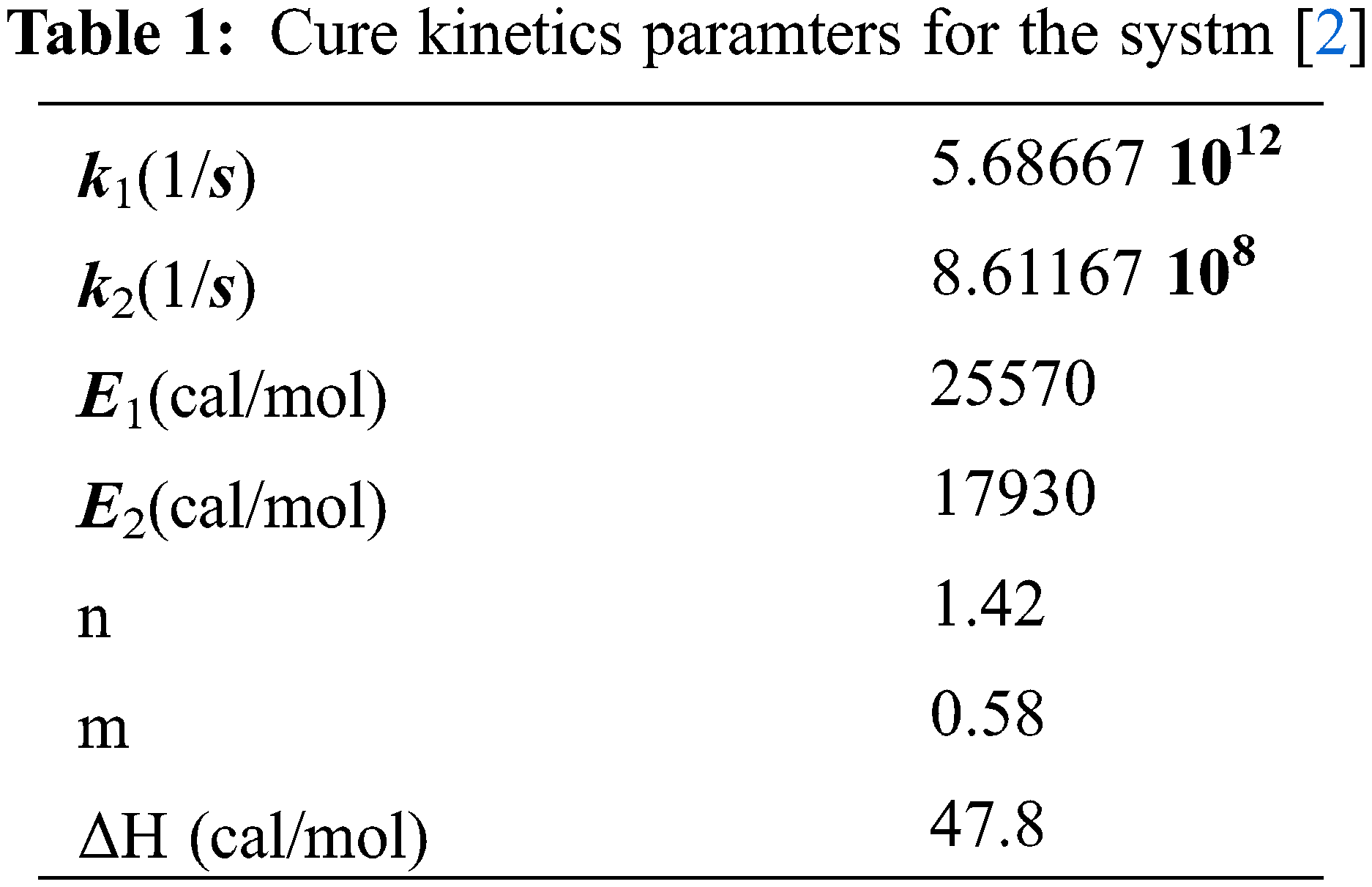
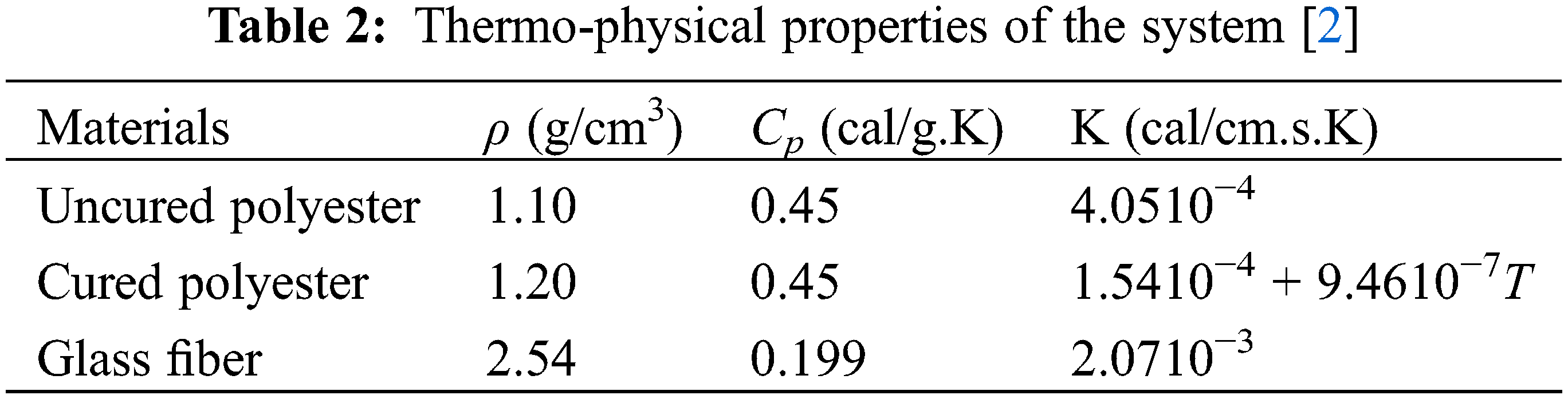
In this study we have considered a mold with rectangular shape as it is presented in Fig. 1. We have opted for glass fiber impregnated with polyester resin. The cure kinetics paramters and the thermo-physical properties of the system used are presented respectiveley in Tables 1 and 2.
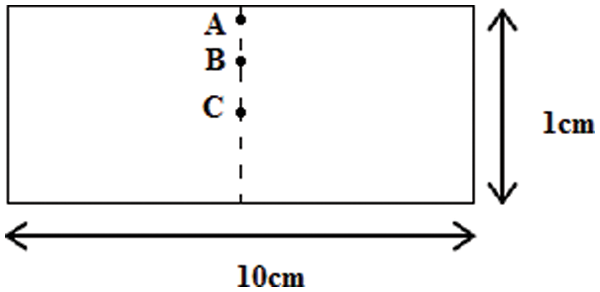
Figure 1: Mold configuration point with studied points: A, B and C
The numerical model that we developed for the polyester resin and fiber glass system is based on the resolution of the energy equation and the degree of the curing reaction. This coupling allows us to determine both the temperature and the degree of curing α (T, α) at each point in the thickness laminate in the mold and at each moment [6], this allows to understand the evolution of the chemical kinetics of the resin.
From the results illustrated in Figs. 2 and 3 we can observe that the temperature and the degree of cure develops very quickly in the center of the Polyester/Glass composite which causes an exothermic peak, this agree well with the results of Choi et al. [2].
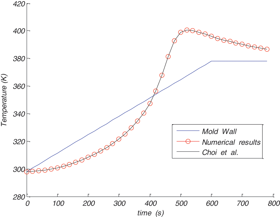
Figure 2: Temperature variation at the laminate centre
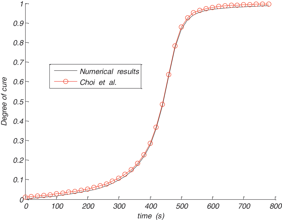
Figure 3: Degree of cure at the centre of the composite
One can deduce from the Fig. 2 that the maximum value of temperature is 400.27 K wheareas its value did not exceed 378 K in the mold wall.
4.2 Procedure to Reduce Thermal Gradients
In almost all of the applications we use one ply of reinforcement with uniform properties, but in the case of low thermal conductivity the thermal gradient is highly pronouced, to resolve this situation one can increase the conductivity of the whole reinforcement, which is not practical since it increases the cost of the final product. To overcome this restriction we have suggested to use a multiple plies of reinforcement (Three plies) (Fig. 4) and we then choose a high conductivity for only the middle ply because of the thermal gradient is higher at the center of the composite according to Choi et al. [2].
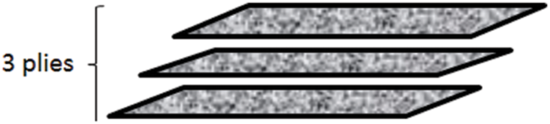
Figure 4: Three reinforcement layer model
• Multiple plies reinforcement
The Table 3 gives the thermo-physical properties of the materials used in our simulation.
Case 1: Same nature of reinforcement
By our numerical sudy, we first used the fiber glass in the three layers with the conductivity is higher at the center. Fig. 5 gives the temperature variation at the different points (A, B, C) in the thikeness of the laminates, as it is shown we can deduce that the thermal gradient is reduced considerably.
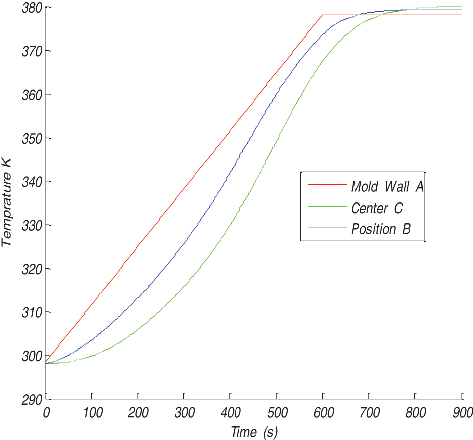
Figure 5: Profile of temperature in different thikeness position of the preform
From Fig. 6, we can see observe at the beguining of curing that the degree of curing at the center is low, this is due to the low temperature in this region of the composite; nevertheless, the curing degree increased suddenly when the temperature increased due to the resin exothermic reaction.
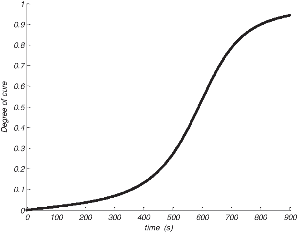
Figure 6: Degree of cure at the centre of the laminate
In this case by using fiberglass the gradient is considerably reduced and the maximum temperature is 379.8103 K and the degree of cure reaches 0.96.
By changing the nature of fiber, we noted that the thermal gardients has slightly changed, in fact, the maximun temperature was 379.7801 K in aramide and 379.6887 with carbone.
To more increase the degree of cure in the case of fiberglass in order to guarantee a complete reticulation for the composite. We increase the temperature of the mold wall to 390 K, and contrary to what can happen in the normal condition, the temperature does not surpass its value on the mold borders (Fig. 7), in addition no gradient appears, and the curing is complete, the degree of cure is almost 1 (Fig. 8).
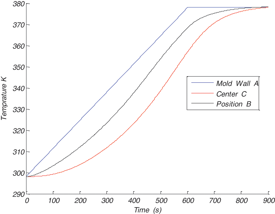
Figure 7: Temperature variation at three different position of the reinforcement in the three plies of the laminate with the mold wall temperature 390 K
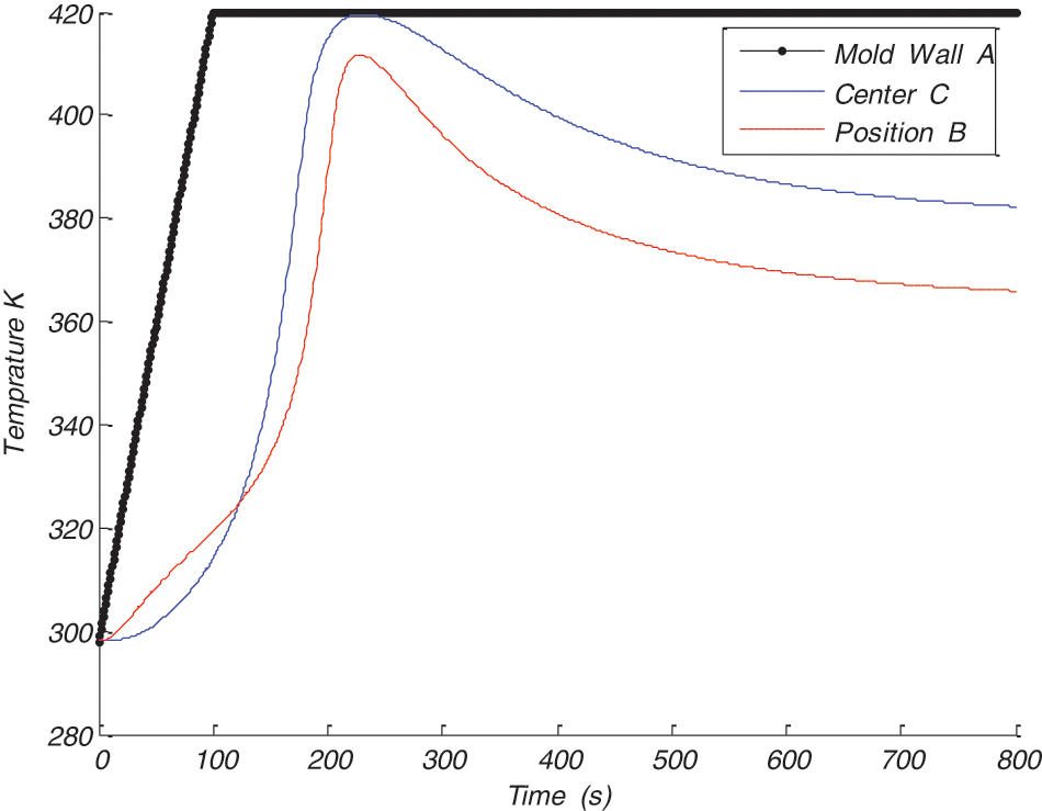
Figure 8: Temperature variation in different position of the reinforcement
Case 2: Differents nature of reinforcement
In the other hand, and by using the mold wall tempertaure 378 K, when we combine between aramide and glass fiber (i.e., the inner ply is in aramide and the two extenal plies are in fibergalss), we obtain the minimun gradient of 379.65 K by comparison with using only glass or aramide or carbone in the three plies of the reinforcement.
• Optimization effect of the temperature cycle
El Yousfi et al. [10] have studied the effect on thermal gradient of differentes variables like fiber type, resin type, and they concluded that the control of the temperature distribution is possible if these parameters were carefully chosen.
Elsemore, it was proved by many researches [2,10] that the temperature cycle play an important role on the curing process. The big deal is to find of an optimum temperature cycle to ensure a full resin cure.
A series of numerical modeling was carried out for differentes possible scenarios, this allows us finally to opte for a particular temperature cycle (Fig. 8) with a good resin cure and the most important with a minimum gradient as it is shown in Fig. 9.
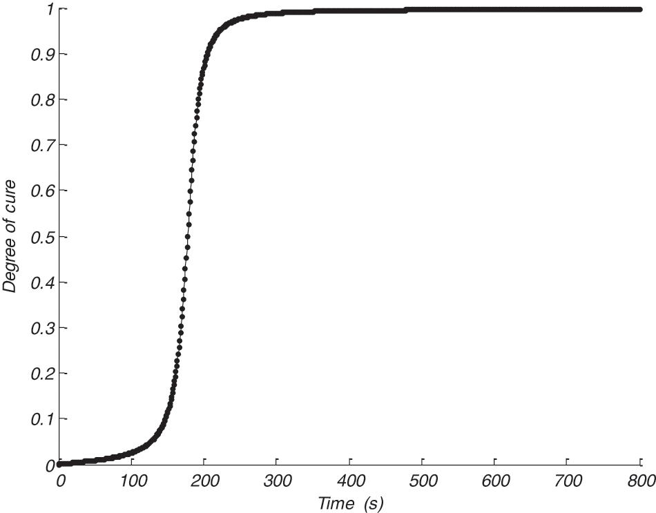
Figure 9: Degree of curing α at the centre of the reinforcement
We can observe from Fig. 9 that with a mold wall temperature of 420 K, the maximun temperature was 420.1745 K and the degree of cure reaches 0.99 in the composite; this ensure a good and entire polymerisation of the whole composite.
In this numerical sudy, we have opted for the explicit finite difference methods in the one-dimensional case applied to composite laminate. The developped program allows us to determine both the coupled temperature and the degree of curing in the composite. Furthermore, and following particular strategies, namely the best selection of fiber and reinforcement structure and the judicious control of the imposed temperature, we have shown that the thermal gradient could be reduced by a big margin. We have proved that our numerical results agree well with some experimental and numerical results in the litterature.
The obtained results prove that our numerical method permit to reduce the thermal gradients effeciently in composite pieces produces by resin transfer molding. This study can afford a robust tool to help engineers and designers in manufacturing composite with good mechanical performace.
Funding Statement: The authors received no specific funding for this study.
Conflicts of Interest: The authors declare that they have no conflicts of interest to report regarding the present study.
References
1. Saad, A., Echchelh, A., hattabi, M., El Ganaoui, M. (2011). An improved computational method for non isothermal resin transfer moulding simulation. Thermal Sciences, 15, 275–289. DOI 10.2298/TSCI100928016S. [Google Scholar] [CrossRef]
2. Choi, M. A., Lee, M. H., Lee, S. J. (1998). Numerical studies during cure in the resin transfer molding. Korea Polymer Journal, 6, 211–218. [Google Scholar]
3. Vincenza, A., Michele, G., Hsiao, K. T., Suresh, G. A. (2002). A methodology to reduce thermal gradients due to the exothermic reactions in composites processing. International Journal of Heat and Mass Transfer, 45, 1675–1684. DOI 10.1016/S0017-9310(01)00266-6. [Google Scholar] [CrossRef]
4. Cheung, A., Yu, Y., Pochiraju, Y. (2004). Three-dimensional finite element simulation of curing of polymer composites. Finite Elements in Analysis and Design, 40, 895–912. DOI 10.1016/S0168-874X(03)00119-7. [Google Scholar] [CrossRef]
5. Kim, J. S., Lee, D. G. (1997). Development of an autoclave cure cycle with cooling and reheating steps for thick thermoset composite laminates. Journal of Composite Materials, 31, 2264–2282. DOI 10.1177/002199839703102203. [Google Scholar] [CrossRef]
6. Bogetti, T. A., Gillespie, J. W. (1992). Process-induced stress and deformation in thick-section thermoset composite laminates. Journal of Composite Materials, 26, 627–660. DOI 10.1177/002199839202600502. [Google Scholar] [CrossRef]
7. Bogetti, T. A., Gillespie, J. W. (1991). Two-dimensional cure simulation of thick thermosetting composites. Journal of Composite Materials, 25, 239–273. DOI 10.1177/002199839102500302. [Google Scholar] [CrossRef]
8. Goncalvès, E. (2005). Resolution numérique, discretisation des EDP et EDO. Institut National Polytechnique de Grenoble. [Google Scholar]
9. Kamal, M. R., Sourour, S. (1973). Kenitics and thermal characterization of thermoset cure. Polymer Engineering and Science, 13(1), 59–64. DOI 10.1002/pen.760130110. [Google Scholar] [CrossRef]
10. El Yousfi, S., Saad, A., Echchelh, A., Hattabi, M. (2020). Thermal characterization and improvement of curing stage in resin transfer molding process. In: Handbook of research on recent developments in electrical and mechanical engineering. DOI 10.4018/978-1-7998-0117-7.ch018. [Google Scholar] [CrossRef]
 | This work is licensed under a Creative Commons Attribution 4.0 International License, which permits unrestricted use, distribution, and reproduction in any medium, provided the original work is properly cited. |