DOI:10.32604/iasc.2020.011688
| Intelligent Automation & Soft Computing DOI:10.32604/iasc.2020.011688 | |
| Article |
SRI-XDFM: A Service Reliability Inference Method Based on Deep Neural Network
1State Key Laboratory of Networking and Switching Technology, Beijing University of Posts and Telecommunications, Beijing, 100000, China
2The 54th Research Institute of CETC, Shijiazhuang, 050000, China
*Corresponding Author: Yang Yang. Email: yyang@bupt.edu.cn
Received: 23 May 2020; Accepted: 10 July 2020
Abstract: With the vigorous development of the Internet industry and the iterative updating of web service technologies, there are increasing web services with the same or similar functions in the ocean of platforms on the Internet. The issue of selecting the most reliable web service for users has received considerable critical attention. Aiming to solve this task, we propose a service reliability inference method based on deep neural network (SRI-XDFM) in this article. First, according to the pattern of the raw data in our scenario, we improve the performance of embedding by extracting self-correlated information with the help of character encoding and a CNN. Second, the original sum pooling method in xDeepFM is improved with an adaptive pooling method for reducing the information loss of the pooling operations when learning linear information. Finally, an inter-attention mechanism is applied in the DNN to learn the relationship between the user and the service data when learning nonlinear information. Experiments that were conducted on a public real-world web service data set confirm the effectiveness and superiority of the SRI-XDFM.
Keywords: Web service; reliability inference; recommendation system; deep neural network
With the rapid development of the Internet, the number of web services has exploded. Many of these massive services provide similar or identical functions [1]. In order to reduce the difficulty when users choose web services, service reliability inference is becoming a key instrument in web service recommendation.
As a method that can recommend specific products to specific users, the recommendation system can be applied to the service reliability inference problem. The xDeepFM [2] model is an outstanding deep neural network recommendation model, which saves the trouble of manually performing feature engineering in the traditional recommendation system. It also solves the dimensional disaster problem caused by the sparse features, which is a common issue in recommendation systems.
As a general model, xDeepFM has the following disadvantages in the service reliability inference scenario. Firstly, the embedding layer of the xDeepFM model consists of a one-hot coding part and a fully-connected layer, which is called the random initialization method [3]. However, there are fields such as the IP addresses and URLs in the raw data that are self-correlated. If the URLs of two services have similar spellings, they are more likely to have a certain relationship. We call that kind of relationship the distance between elements. The random initialization method of xDeepFM will completely destroy such distance information. Due to the characteristic of one-hot coding, the completely discarded distance information will no longer been learned in subsequent works. Secondly, in the xDeepFM model, in order to imitate the traditional collaborative filtering method to extract features, a CIN model is proposed and applied. CIN can effectively extract the high-dimensional features in the data. However, it utilizes a sum pooling [4] method to reduce the dimension, which can easily lose a host of information. Thirdly, in order to extract the nonlinear bit-wise feature in the raw data, a DNN is adopted. However, its structure is rather simple. The data of users and services are simply flattened into a vector as the input, without considering the relationship between users and services.
In order to solve above disadvantages of the xDeepFM model in our certain scenario, this paper proposes a service reliability inference method based on the xDeepFM model and it is summarized as follows.
According to the pattern of raw data, the embedding layer is improved. Self-correlated information such as the IPs and URLs are extracted from all the fields. Afterwards, a character encoding method is applied to replace the original one-hot encoding method. In addition, the encoded fields are put into a CNN to preserve the distance between elements.
The CIN model is improved using a favorable pooling method. This paper replaces the original sum pooling method with the proposed adaptive pooling method and proposes an A-CIN network. Thus, the pooling operation reserves more information with the same shape, which improves the performance of the explicit knowledge learning.
An inter-attention method is proposed to improve the performance of the DNN. This paper introduces an attention mechanism into the DNN model and proposes an A-DNN network. This method performs an interactive operation between the user and service features, which can concentrate the model’s attention on the relevant fields, and improves the model’s ability to learn implicit information.
The rest of this article is organized as follows. Section 2 reviews some related works. Section 3 describes our service reliability inference method, which is named SRI-XDFM. The simulation results and corresponding discussions are presented in Section 4. Finally, Section 5 summarizes this paper.
2.1 xDeepFM: Combining Explicit and Implicit Feature Interactions for a Recommender System
In the recommendation system, feature engineering plays a vital role [5]. In feature engineering, mining cross features is crucial. Cross features refer to cross combinations between two or more original features. As an example, a three-dimensional intersection feature is AND (User IP = 12.108.127.138, User Country = United States, Service IP = 8.23.224.110), which means that the current user’s IP address is 12.108.127.138, the country is The United States and the IP address of the current service is 8.23.224.110. In the traditional recommendation system, mining cross features mainly depends on manual extraction [6]. This method has three shortcomings:
1) The labor cost is high;
2) A large number of sparse features easily brings about the dimensional disaster problem;
3) Manually extracted cross features cannot be generalized to patterns that have never appeared in training samples.
Therefore, it is extremely meaningful to automatically learn the interactions between features. At present, most of the related research work is based on the factorization machine framework [7], which utilizes a multi-layer fully connected neural network to automatically learn the high-order interaction between features. The disadvantage is that the model learns implicit interaction features whose form is unknown and uncontrollable. At the same time, their feature interaction occurs at the element level rather than between feature vectors, which violates the original intention of the factorization machine. xDeepFM [2] is a model that solves the above problems. It learns both bit-wise and vector-wise features in both explicit and implicit ways.
Bit-wise and Vector-wise: Assume that the dimension of the hidden vector is 3. Also assume that there are two features,  and
and  . When the features interact in the form similar to
  , we say that feature interaction occurs at the bit-wise level. If the form of the feature interaction is similar to
  , then we say that feature interaction occurs at the vector-wise level.
Explicitly and Implicitly: Given two features  and
and  , after a series of transformations, if the output can be described in the form of
  , we say that it is explicit feature interaction. Otherwise, it is implicit feature interaction.
By combining a CIN model with a linear regression unit and a fully connected neural network, we get the final model and name it the Explicit and Implicit Deep Factorization Machine (xDeepFM).
There have also been some methods to predict or select web services. In 2019, Poordavoodi, Alireza et al. modified the Interval Data Envelopment Analysis Models for QoS-aware Web service selection considering the uncertainty of QoS attributes in the presence of desirable and undesirable factors. It improved the fitness of the resultant compositions when they filter out unsatisfactory candidate services for each abstract service in the preprocessing phase [8]. Yang, J proposed a Network Risk Evaluation model using deep learning. It presented a mechanism of sharing hyper-parameters to improve the efficiency of learning and a hierarchical evaluative framework for Network Risk Evaluation [9]. In 2020, Muhammad Hasnain et al. proposed a performance anomaly detection in web service that uses dynamic features of quality of service that are collected in a simulated setup. Three variants of recurrent neural networks: SimpleRNN, long short term memory, and gated recurrent unit were evaluated [10].
2.2 CIN: Compressed Interaction Network
In order to realize the automatic learning of explicit high-order feature interactions and at the same time make the interactions occur at the vector level, xDeepFM proposes a new neural network called the Compressed Interaction Network (CIN). In the CIN, the hidden layers are called the unit objects. The original features of the input together with the output of the unit objects are organized into matrixes, which are denoted as  and
and  . The output of each unit object
  is derived from the previous layer’s output
  and the original feature vector
  .
.
The  hidden layer contains
  neuron units. The calculation of the hidden layer can be divided into two steps.
(1) According to the state  of the previous hidden layer and the original feature matrix
  , calculate an intermediate result
  , which is a three-dimensional tensor.
(2) Based on this intermediate result,  intermediate layers with a size of
  are used to generate the state of the next hidden layer. This operation is similar to the idea of a convolutional neural network. However, the “Feature Map” obtained in the CIN is a vector, not a matrix. The final “Feature Map” is determined by all of the layers of the network, and each hidden layer is connected to the output layer through a sum pooling operation.
The encoder-decoder model is a solution to the seq2seq problem [11]. The fatal limitation of this model is that the single connection between the encoder and decoder is a fixed-length semantic vector C. In other words, the encoder will compress the entire sequence of information into a fixed-length vector. There are two drawbacks. Firstly, the fixed semantic vector cannot fully represent the information of the entire sequence. Secondly, the information carried by the first input will be diluted by the information entered later. The longer the input sequence is, the more serious this phenomenon.
In order to solve this problem, the author of [12] proposed the idea of Attention. When this model generates an output, it also generates an “attention range” that indicates which parts of the input sequence should be focused on when outputting, and it then generates the next output based on the area of interest.
Compared with the previous encoder-decoder model, the biggest difference of the attention model is that it does not require the encoder to encode all input information into a fixed-length vector. In addition, during decoding, each step will respectively select a subset of the vector sequence for further processing. In this way, when each output is generated, the information carried by the input sequence can be fully utilized. Furthermore, this method has achieved very good results in translation tasks.
In essence, attention selectively filters out a small amount of important information from a large amount of information and focuses on this important information [13]. The process of focusing is reflected in the calculation of the weight coefficient. The larger the weight is, the greater the focus on it.
3 SRI-XDFM: The Proposed Service Reliability Inference Method
We propose a new service reliability inference method named the Service Reliability Inference Method based on Deep Neural Network (SRI-XDFM), with the following considerations.
(1) Self-correlated features are embedded according to the distance between features rather than randomly;
(2) The pooling of the feature map is adaptive, which means that the output can contain more information, and
(3) The relationship between the user and service fields is concentrated in the process of non-linear knowledge learning.
The basic workflow of the SRI-XDFM is shown in Fig. 1 and described as follows.

Figure 1: The structure of the SRI-XDFM
There are three main processes in the SRI-XDFM: embedding, the A-CIN and the I-DNN.
In the next sections, we will introduce these three important units.
3.2 Embedding for Self-Correlated Data
The original data are divided into two parts according to if they belong to a user or a service. Then, these two parts are further classified according to the field. A field here refers to the one-dimensional input in the original data. For example, the country to which the user belongs is a field. Afterward, all the field data are divided into two parts according to if it is self-correlated. A self-correlated field here refers to a field with the following characteristic: The distance between two instances that are picked arbitrarily from the field contains valid information. For example, the user’s IP address is a self-correlated field since we can say that two users are related somehow if the IP addresses of these users are similar. On the contrary, the country to which the user belongs is a non-self-correlated field since there contains little useful information in two countries whose spelling is similar.
The fields that are classified and named  and
and  are the input of the embedding layer. For fields that are non-self-correlated, the random initialization method is utilized as with the original xDeepFM. Firstly, the one-hot encoding method is applied to each field. For example, suppose that there are three kinds of data in the country domain: China, the United States, and the United Kingdom. Then encode China as (0, 0, 1), encode the United States as (0, 1, 0), and encode the United Kingdom as (1, 0, 0). After encoding, enter the vectors into a fully connected layer and each field is converted into a vector of length D. Then, for the fields that are self-correlated, they are encoded with a character method and put into a CNN. The overview of the embedding layer is shown as Fig. 2.

Figure 2: The structure of embedding
One-hot encoding is a method that encodes the input only based on the classification of raw data [14]. Hence, it introduces two issues into our scenario.
Firstly, the relationship between two inputs is discarded in the random encoding process as we mentioned before. Thus, it can never be learned in the next steps in the model. That means that we lose some information from the original data that is of vital importance.
Secondly, the content of some fields in the original data is too sparse. For example, users will seldom share the same IP address. Therefore, this field will be encoded into a rather long vector, which is unacceptable.
To solve the above problems, we introduce a character encoding method to the embedding layer to replace the one-hot method for self-correlated data. The raw data are encoded in a character way according to specific business scenarios. For example, the IP address of a user is 12.108.127.138, and the corresponding binary IP address is 00001100, 01101100, 01111111, and 10001010. This 32-dimensional variable is the character encoding vector of this user’s IP field. Another scenario is the encoding of the URLs. Suppose that a service has the URL with the path www.abc.com. We firstly encode the English letters in order. A is encoded as 1, B is encoded as 2 and so on. Then, we can encode the URL as 23,23,23,1,2,3,3,15,13. All the URLs are encoded to a certain length whose value equals the length of the longest URL in the dataset. Extra bits will be encoded as zeros.
Character encoding is a method that ensures the important self-correlated information will not be discarded. However, we need a method to transfer raw data with different shapes and rather long sizes into embedding features with a certain shape not taking up too much space. Furthermore, the self-correlated information should be extracted in a reasonable way. Therefore, we adopt a Convolution Neural Network (CNN), which does a good job on the above statements.
The CNN is a feed forward neural network, which extracts hidden local correlation features via the layer-by-layer convolution and pooling of input data, and generates high-level features via layer-by-layer combination and abstraction [15]. As we all know, the CNN has made great success in the field of image classification, and there are two patterns in user and service data similar to that of an image. Firstly, there are some patterns smaller than the whole data. Secondly, the same patterns appear in different regions. Although a CNN can effectively extract the pixel information of two-dimensional images, however, the features in our scenario are one-dimensional. Therefore, we use a one-dimensional convolution kernel instead. In this way, the self-correlated information extraction process we expect to realize in this paper is very similar to the pixel information extraction process of images.
The CNN model designed for embedding feature extraction in this paper consists of two convolution layers, two max pooling layers, and two fully connected layers.
Convolution layer: The model contains two convolutional layers C1 and C2. The function of the convolutional layer is to use filters (convolution kernels) to slide in the input data and perform a convolution weighting operation to complete feature extraction. Different filters can extract different features. In C1, a raw vector is transformed into 3 feature maps with a length smaller than the raw vector by 2. In C2, the operation is bounded with the depth of the pooled vector. The adopted activation function after each convolutional layer is the “ReLu.”
Pooling layer: The pooling layer is the lower sampling layer in a CNN. And it is used to reduce the dimension, shorten the training time and control over fitting. The most common pooling types are max pooling and mean pooling. This paper uses max pooling to retain more significant information. The size of the convolution kernel of the pooling layer is set to 2.
Dense layer: The output of P2 is three pooled vectors. After being flattened, they are transformed to a long vector, which is the input of the dense layer. The main purpose of the dense layer is to extract the distinguishing features by combining and sampling the features extracted from the convolutional layer, and it finally achieves the purpose of embedding. It has two fully connected layers to extract features into an embedding vector with a size of D. The activation function is also the “ReLu.”
3.5 A-CIN: Improved CIN Using Adaptive Pooling
The Adaptive Compressed Interaction Network (A-CIN) is a neural network with the purpose of extracting vector-wise information and learning knowledge implicitly. It takes advantage of the idea of the factorization machine and solves the problem of how to combine features in the case of sparse features. The overview of the A-CIN is shown in Fig. 3.

Figure 3: The structure of the A-CIN model
After embedding, all user and service data are converted into x and y vectors with a length of D. We reconstruct them into a matrix that is the input of the A-CIN. Then, it is applied to k operations similar to feature map extraction and named compression, whose purpose is to combine the features on the vector-wise level and simulate the factorization machine. Each output of the compression is passed to an adaptive pooling method. All the output of the adaptive pooling is flattened into a vector, which is the output of the A-CIN.
We combine all user and service embedding vectors into a matrix  , where
  . The
. The  row in
  is the embedding vector of the
  field. The output of the
  layer in A-CIN is also a matrix
  , where
  denotes the number of feature vectors in the
  layer and we let
  . For each layer,
  is calculated via the following:

Here  is the parameter matrix for the
  feature vector, and
  denotes the Hadamard product as follow:

Note that  is derived via the interactions between
  and
and  . Thus feature interactions are measured explicitly, and the degree of interactions increases with the layer depth. We hold the structure of the embedding vectors at all layers, and thus the interactions are applied at the vector-wise level.
The purpose of adaptive pooling is to reduce the dimension of the output of the compression and reserve more information at the same time. Every hidden layer  , where
  , has a connection with output units. For example, we select a vector in H, and it is denoted as
  . The overview of adaptive pooling is shown in Fig. 4.

Figure 4: The structure of adaptive pooling
The output of adaptive pooling is a number y. With that in mind, we firstly combine all units of H and then put them into a neural-like structure, which results in s. It is calculated as follows:

Note that it is not a neural network for all the parameters  here is not determined by learning, but is dynamically determined. That means we can only know its value after we put data in the model and start the process online, which is same as max pooling.
Then, s is the input to an operation called resize, which aims to restrict all the s with a certain scope. The output is denoted as a and calculated as follows:

Then, we can get a vector B denoted as  , which is calculated via the following:

The above is one iteration in the algorithm. After several iterations, we can get the output. Here we conduct 3 iterations. The process is shown in Algorithm 1.
Algorithm 1: The Adaptive Pooling Algorithm
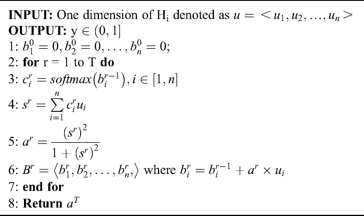
Afterwards, all outputs of adaptive pooling are flattened to a vector as the output of the A-CIN layer.
3.8 I-DNN: Improved DNN Based on Attention Mechanism
The inter-attention Deep Neural Network (I-DNN) is a model that runs parallel to the A-CIN. A kind of attention mechanism is applied here to concentrate on the relationship between user and service information. Firstly, we construct the user and service embedding vectors into two matrixes. Secondly, they are put into an inter-attention layer. The output is a vector that contains the user and service attention information. Finally, they are put into a DNN to extract bit-wise knowledge. The overview of the I-DNN is shown in Fig. 5.

Figure 5: The structure of the I-DNN model
The output of all embedding layers is divided into two categories, namely, user and service features. We construct these vectors as two matrixes named  and
and  , where the
  vector of A or B is the
  user or service feature. A and B are the inputs of the inter-attention layer and the output is a vector, named P.
Firstly, we construct a matrix  with A and B. Each element of E is denoted as
  and calculated via the following:

Here  contains the relationship of the local sequences between A and B.
Secondly, we reconstruct two matrixes, named  and
and  , where the
  vector of A and the
  vector of B are denoted as
  and
and  , respectively, which are calculated via the following:
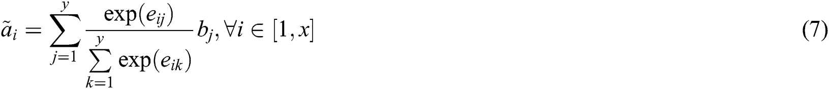
Thirdly, we flatten A and B to P, which is the output of the Inter-attention layer. Thus the input of the DNN is P, which contains relationship information instead of straight flattening A and B to a plain vector.
Finally, we put P into the DNN. Here we put three hidden layers inside with the “ReLu” activation function, after which we get a vector named V. That is the output of the I-DNN layer.
4 Performance Evaluation Results
4.1 Experimental Environment and Data Set
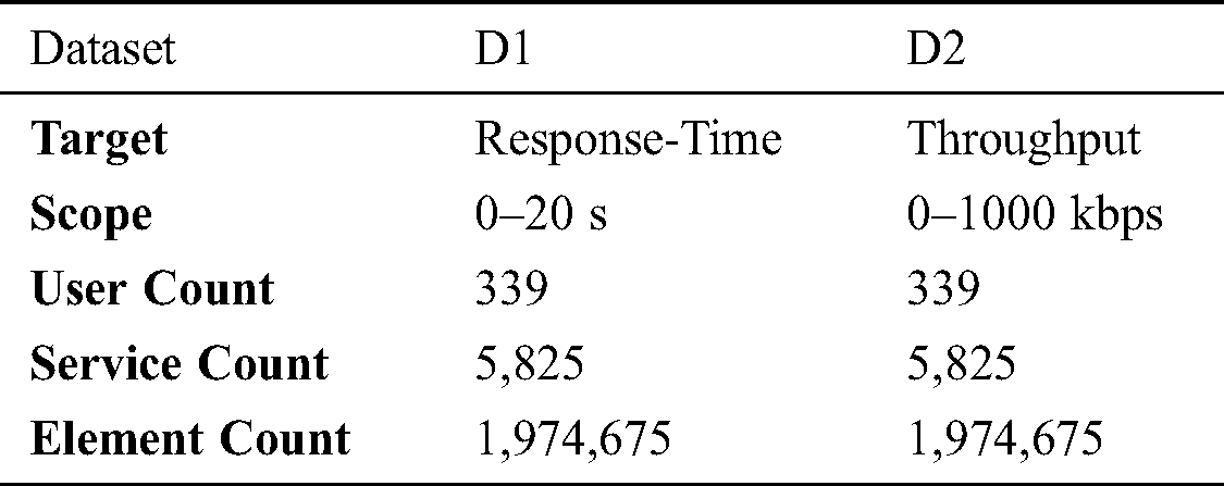
A real-world web service performance dataset (WSDREAM) [16] is employed for experiments, and the details are summarized in Tab. 1. As shown, they include the response time and throughput on 5825 real-world web services experienced by 339 users. Both datasets contain 1,974,675 records each. In a real case, the amount of information that we know is rather lower. Hence, in the experiments, we adopt a small part of the dataset, that is, 20%–40%, to train the model, and predict the remaining 80%–60% of the data to evaluate the performance.
Here we define the reliability of a service between user  and server
  as
as  , which is calculated via the following:


 and
and  denote the scores of the response time and throughput between
  and
and  , respectively.
  and
and  denote the values of the response time and throughput between
  and
and  , respectively.
The experimental environment in this paper is a server with 8G of memory and a 1.6 GHz CPU (Xeon e5–2603 v3). All the algorithms are written in the Python 3.7 environment using the Keras library and scikit-learn tools.
We adopt the mean absolute error (MAE) and the root mean square error (RMSE) as the performance measurements for our model [17].
The MAE is defined as follows:

Here  denotes the real reliability value of service i observed by user u.
  denotes the predicted reliability value, and N denotes the number of predicted values.
The RMSE is defined as follows:

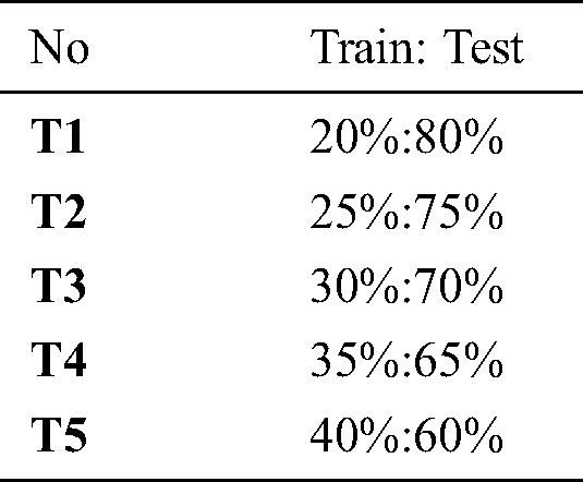
We compare the performance of the SRI-XDFM with four models that are able to perform service reliability inference, including the NNMF [18,19], TSVD [20], WSPM [21] and xDeepFM [2]. For both datasets, we design five testing cases, whose details are given in Tab. 2.
We evaluate the performance of our proposed method from four aspects: The general model effect, the effectiveness of the self-correlated feature embedding, the effectiveness of the adaptive pooling and the effectiveness of the inter-attention mechanism.
4.3.1 The General Model Effect
General model means the proposed model that combines self-correlated feature embedding, adaptive pooling and the inter-attention mechanism.
We evaluate the overall result of our model here. The evaluation of the general model is shown as follows.
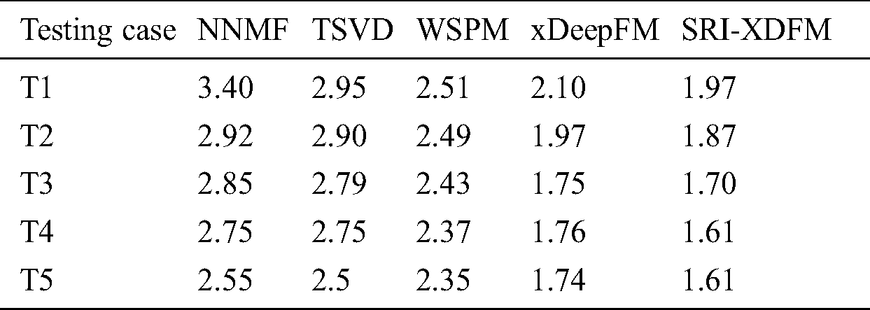
Tab. 3 shows the comparison of the MAEs among the other four models and the SRI-XDFM. It can be seen that the SRI-XDFM gets the best MAE in every testing case. When using testing case T1, its MAE is 72.5%, 49.7%, 27.4% and 6.6% better than those of the NNMF, TSVD, WSPM and xDeepFM, respectively. When using testing case T5, its MAE is 58.4%, 55.3%, 45.9% and 8.1% better than those of the NNMF, TSVD, WSPM and xDeepFM, respectively. We can find that when the amount of training data is less, the SRI-XDFM performs better. That is similar to the condition in the real world.
Table 3: The general model MAE comparison
Tab. 4 shows the comparison of the RMSEs among the other four models and the SRI-XDFM. It can be seen that the SRI-XDFM also gets the best RMSE in every testing case. When using testing case T1, its RMSE is 46.2%, 33.8%, 17% and 6.2% better than those of the NNMF, TSVD, WSPM and xDeepFM, respectively. When using testing case T5, its RMSE is 33.6%, 32.5%, 15.2% and 0.8% better than those of the NNMF, TSVD, WSPM and xDeepFM, respectively. We can also find that when the amount of training data is less, the SRI-XDFM performs better.
Table 4: The general model RMSE comparison
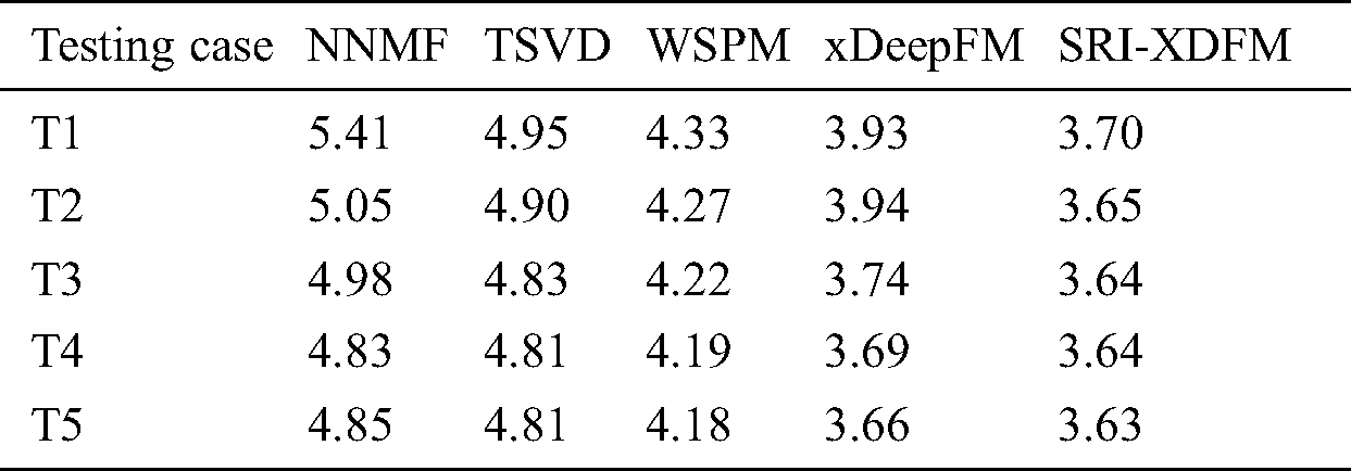
Fig. 6 shows the line charts of the general model effect comparison. It can be found that when the amount of training data increases and the amount of testing data decreases, all the models’ MAEs and RMSEs decline with different patterns. The NNMF model shows an unstable and steep curve and gets the worst result, which are respectively 72% and 46% worse than those of the SRI-XDFM when using testing case T1. The TSVD model’s performance is similar to that of the NNMF, but it gets rather better scores when the training set is small. The WSPM model is the most stable and gets better scores than the above two models. As our base model, xDeepFM performs much better than the other three models in both the MAE and RMSE. Our proposed model, the SRI-XDFM shows the best performance among all.

Figure 6: The general model effect comparison (a) MAE (b) RMSE
Overall, compared with the other four models, the SRI-XDFM is 20.27%, 13.02%, 7.16% and 4.55% better in the MAE and 5.6%, 3.21%,1.32% and 0.14% better in the RMSE. Therefore, we can say that the general model shows great superiority, and the task of service reliability inference is better solved. It is of great significance for service selecting in real world.
4.3.2 The Effectiveness of the Proposed Methods
In this section, we evaluate the effectiveness of self-correlated feature embedding, adaptive pooling and the inter-attention mechanism by comparing the original xDeepFM with a xDeepFM plus a self-correlated feature embedding part, a xDeepFM utilizing adaptive pooling instead of max pooling and a xDeepFM plus an inter-attention layer. Hereafter, we call them the S-XDFM, A-XDFM and I-XDFM, respectively.
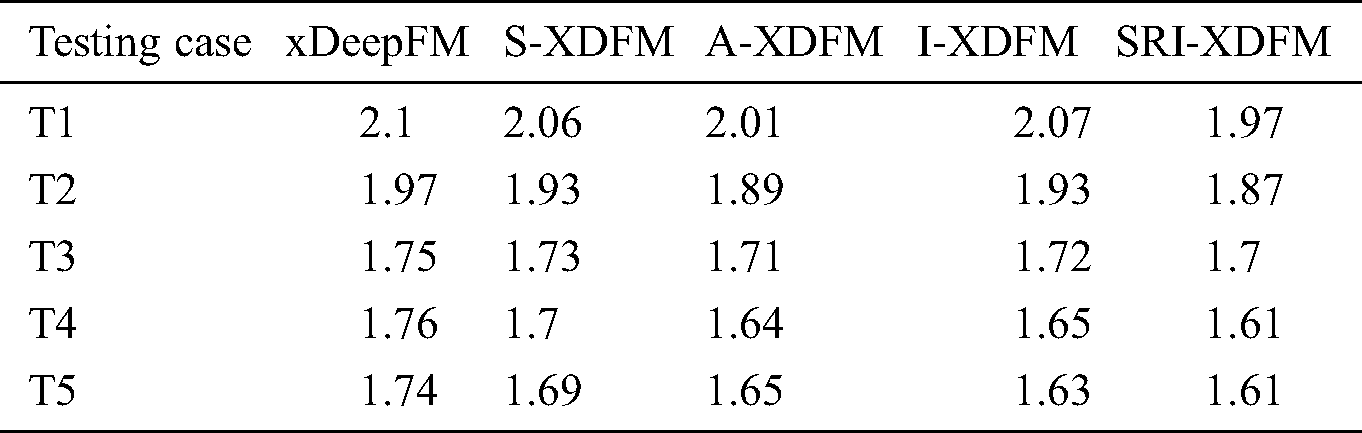
Tab. 5 shows the comparison of the MAEs of the proposed methods. When testing case T1 is used, the A-XDFM gets the best MAE, and it is smaller than the other two by 0.5 and 0.6, respectively. The S-XDFM and I-XDFM shares similar bad results. When testing case T5 is used, the I-XDFM gets the best value, and its MAE is smaller than the other two by 0.02 and 0.07, respectively. The performance of the A-XDFM is not as good as it was with T1. The S-XDFM still gets a bad result. It can be seen that when the amount of training data is small, it would be good to adopt the adaptive pooling method. However, when the size of the training set increases, the inter-attention method will play an increasingly more important role in the MAE evaluation.
Table 5: Comparing the MAEs of the proposed methods
Tab. 6 shows the comparison of the RMSE of the proposed methods. When testing case T1 is used, the S-XDFM gets the best RMSE, and its RMSE is smaller than the other two by 0.26 and 0.23, respectively. The A-XDFM and I-XDFM shares similar bad results. When testing case T5 is used, all the three models get similar results. It can be seen that when the amount of training data is small, it would be good to adopt the self-correlated method. However, when the size of training set increases, the differences among them decrease.
Table 6: Comparing the RMSEs of the proposed methods
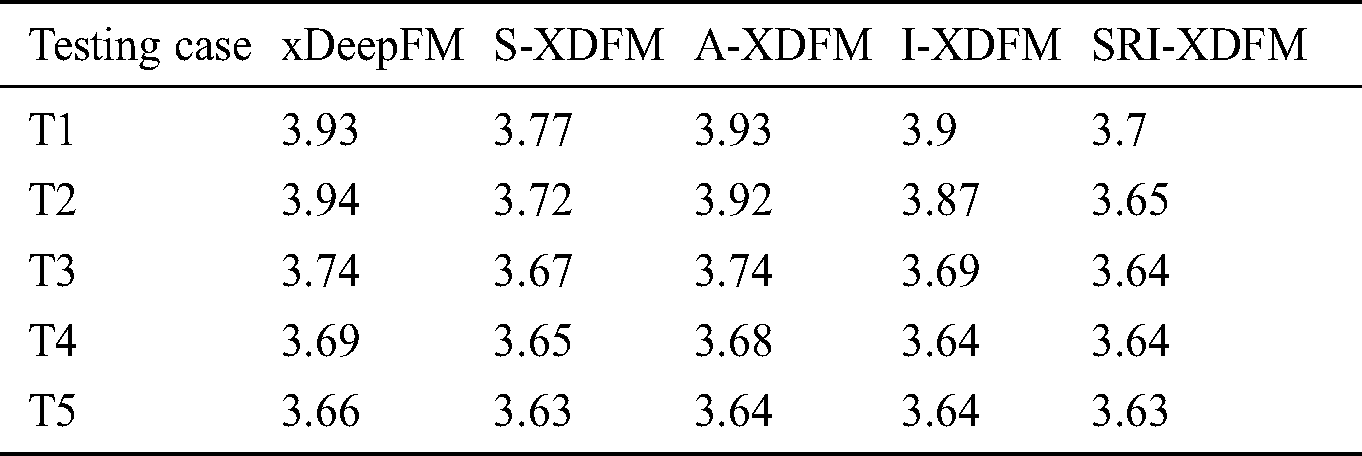
Fig. 7 shows the comprehensive MAEs value and the contributions of the xDeepFM, S-XDFM, A-XDFM, I-XDFM and SRI-XDFM. The contribution is defined as follows:

Figure 7: The comparison of the MAEs of the proposed methods (a) Comprehensiveness (b) Contribution

C represents the contribution value. XD, SRI and T represent the MAE or RMSE of the xDeepFM, the SRI-XDFM and the target model, respectively.
We can see that self-correlated embedding does not have much effect on the general MAE result, and its contribution is only from 30.7% to 40%. Adaptive pooling contributes 69% to 80% to the decrease of the MAE in all testing cases, which means that this method does a great job regarding the MAE. The inter-attention method contributes little when the training set is small at only 23.1%, but it increases sharply with the training set increases and it reaches 84.6% at last.

Figure 8: The comparison of the RMSEs of the proposed methods (a) Comprehensiveness (b) Contribution
Fig. 8 shows that when it comes to the RMSE, all three methods’ contributions obviously increase as the training set gets bigger. Self-correlated embedding’s contribution is from 69.5% to 100% and contributes the most to the curve. Adaptive pooling’s contribution is from 0% to 66.7% and it contributes the least. Inter-attention’s contribution is from 13% to 66.7% and in the middle of the methods. In summary, adaptive pooling does most regarding the MAE and inter-attention does the most regarding the RMSE.
The experimental results show that the combination of these three methods is useful for service reliability inference. When considering both the MAE and RMSE, the inter-attention method gets similar performance. However, it is obviously that the self-correlated embedding method does a better job regarding the RMSE and adaptive pooling is better regarding the MAE.
In summary, all the above experimental results confirm that the SRI-XDFM does a good job in the service reliability inference task and performs better than the other methods.
With the development of web service technology, the number of services on the Internet has exploded. It is of vital importance to select the best service from a vast amount of similar services in a reasonable time. This paper proposes a service reliability inference model called the SRI-XDFM based on a general but effective recommendation system model called xDeepFM. Considering of the pattern of our scenario, three methods are proposed to enhance the effect of our model, including an embedding method addressing the self-correlation pattern in raw data, an adaptive pooling method to reserve more information and an inter-attention method to concentrate on the relationship between user and service. The experimental results show that the proposed method does a good job on this task and it outperforms other models. However, it is far from perfect. This method does not consider time, which is an important factor. Further research can be carried out on this aspect. We hope that our work can provide some references for the service reliability inference research in the future.
Acknowledgement: The authors would like to thank Beijing University of Posts and Telecommunications for the support in this research.
Funding Statement: This work is supported by National Key Research and Development Program of China (2019YFB2103200), the Fundamental Research Funds for the Central Universities (500419319 2019PTB–019), Open Subject Funds of Science and Technology on Information Transmission and Dissemination in Communication Networks Laboratory (SKX182010049), the Industrial Internet Innovation and Development Project 2018&2019 of China.
Conflicts of Interest: The authors declare that they have no conflicts of interest to report regarding the present study.
1. M. Jia, Y. Chen, G. Zhang, P. Jiang, H. Zhang et al.. (2018). , “A web service framework for astronomical remote observation in Antarctica by using satellite link,” Astronomy and Computing, vol. 24, no. 3, pp. 17–24. [Google Scholar]
2. J. Lian, X. Zhou, F. Zhang, Z. Chen, X. Xie et al.. (2018). , “xDeepFM: Combining explicit and implicit feature interactions for recommender systems,” in Proc. of the 24th ACM SIGKDD Int. Conf. on Knowledge Discovery & Data Mining. Association for Computing Machinery, New York, NY, USA, pp. 1754–1763. [Google Scholar]
3. W. Zhang, T. Du and J. Wang. (2016). “Deep learning over multi-field categorical data: A case study on user response prediction,” Lecture Notes in Computer Science, vol. 9626, pp. 45–57. [Google Scholar]
4. Y. Qu, H. Cai, K. Ren, Y. Yu, Y. Wen et al.. (2016). , “Product-based neural networks for user response prediction,” in Int. Conf. on Data Mining, Barcelona, Spanish, pp. 1149–1154. [Google Scholar]
5. A. Elbadrawy and G. Karypis. (2015). “User-specific feature-based similarity models for top-n recommendation of new items,” ACM Transactions on Intelligent Systems, vol. 6, no. 3. [Google Scholar]
6. Y. Koren, R. M. Bell and C. Volinsky. (2009). “Matrix factorization techniques for recommender systems,” IEEE Computer, vol. 42, no. 8, pp. 30–37. [Google Scholar]
7. Y. Xu, R. Hao, W. Yin and Z. Su. (2015). “Parallel matrix factorization for low-rank tensor completion,” Inverse Problems & Imaging, vol. 9, no. 2, pp. 601–624. [Google Scholar]
8. A. Poordavoodi, M. R. M. Goudarzi, H. H. S. Javadi, A. M. Rahmani and M. Izadikhah. (2020). “Toward a more accurate web service selection using modified interval DEA models with undesirable outputs,” Computer Modeling in Engineering & Sciences, vol. 123, no. 2, pp. 525–570. [Google Scholar]
9. J. Yang, T. Li, G. Liang, W. He and Y. Zhao. (2019). “A hierarchy distributed-agents model for network risk evaluation based on deep learning,” Computer Modeling in Engineering & Sciences, vol. 120, no. 1, pp. 1–23. [Google Scholar]
10. M. Hasnain, S. R. Jeong, M. F. Pasha and I. Ghani. (2020). “Performance anomaly detection in web services: An RNN- Based approach using dynamic quality of service features,” Computers, Materials & Continua, vol. 64, no. 2, pp. 729–752. [Google Scholar]
11. S. Xiao, D. He and Z. Gong. (2018). “Deep-Q: Traffic-driven QoS inference using deep generative network,” in Proc. of the 2018 Workshop on Network Meets AI & ML, New York, NY, USA: Association for Computing Machinery, pp. 67–73. [Google Scholar]
12. K. Cho, A. Courville and Y. Bengio. (2015). “Describing multimedia content using attention-based encoder-decoder networks,” IEEE Transactions on Multimedia, vol. 17, no. 11, pp. 1875–1886. [Google Scholar]
13. Z. Zheng and M. R. Lyu. (2010). “Collaborative reliability prediction of service-oriented systems,” in Int. Conf. on Software Engineering, Cape Town, The Republic of South Africa, pp. 35–44. [Google Scholar]
14. T. Katus and M. M. Muller. (2016). “Working memory delay period activity marks a domain-unspecific attention mechanism,” NeuroImage, vol. 128, pp. 149–157. [Google Scholar]
15. C. L. Liu, W. H. Hsaio and Y. C. Tu. (2019). “Time series classification with multivariate convolutional neural network,” IEEE Transactions on Industrial Electronics, vol. 6, no. 6, pp. 4788–4797. [Google Scholar]
16. Z. Zheng and M. R. Lyu. (2008). “WS-DREAM: A distributed reliability assessment mechanism for web services,” in IEEE Int. Conf. on Dependable Systems and Networks with FTCS and DCC, Anchorage, AK, USA, pp. 392–397. [Google Scholar]
17. X. Luo, H. Wu, H. Yuan and M. Zhou. (2019). “Temporal pattern-aware QoS prediction via biased non-negative latent factorization of tensors,” IEEE Transactions on Systems, Man, and Cybernetics, vol. 50, no. 5, pp. 1798–1809. [Google Scholar]
18. S. Zhang, W. Wang and J. Ford. (2006). “Learning from incomplete ratings using non-negative matrix factorization,” in SIAM Int. Conf. on Data Mining, Bethesda, MD, USA, pp. 549–553. [Google Scholar]
19. D. D. Lee and H. S. Seung. (1999). “Learning the parts of objects with non-negative matrix factorization,” Nature, vol. 401, no. 6755, pp. 788–791. [Google Scholar]
20. Y. Koren. (2009). “Collaborative filtering with temporal dynamics,” in Proc. 15th ACM SIGKDD Int. Conf. on Knowledge Discovery, Paris, France: Data Min, pp. 447–456. [Google Scholar]
21. Y. Zhang, Z. Zheng and M. R. Lyu. (2011). “WSPred: A time-aware personalized QoS prediction framework for Web services,” in Proc. 22nd IEEE Int. Sym. on Software Reliability Engineering, Hiroshima, Japan, pp. 210–219. [Google Scholar]
 | This work is licensed under a Creative Commons Attribution 4.0 International License, which permits unrestricted use, distribution, and reproduction in any medium, provided the original work is properly cited. |