DOI:10.32604/iasc.2020.011988
| Intelligent Automation & Soft Computing DOI:10.32604/iasc.2020.011988 | |
| Article |
Deep 3D-Multiscale DenseNet for Hyperspectral Image Classification Based on Spatial-Spectral Information
1School of Electronics and Information Engineering (School of Big Data Science), Taizhou University, Taizhou, 318000, China
2College of Science, Heilongjiang Institute of Technology, Harbin, 150050, China
3Departments of Interactive Technology, Animax Designs, Nashville, 37207, USA
*Corresponding Author: Weiwei Yang. Email: yww_1680@163.com
Received: 09 June 2020; Accepted: 07 July 2020
Abstract: There are two main problems that lead to unsatisfactory classification performance for hyperspectral remote sensing images (HSIs). One issue is that the HSI data used for training in deep learning is insufficient, therefore a deeper network is unfavorable for spatial-spectral feature extraction. The other problem is that as the depth of a deep neural network increases, the network becomes more prone to overfitting. To address these problems, a dual-channel 3D-Multiscale DenseNet (3DMSS) is proposed to boost the discriminative capability for HSI classification. The proposed model has several distinct advantages. First, the model consists of dual channels that can extract both spectral and spatial features, both of which are used in HSI classification. Therefore, the classification accuracy can be improved. Second, the 3D-Multiscale DenseNet is used to extract the spectral and spatial features which make full use of the HSI cube. The discriminant features for image classification are extracted and the spectral and spatial features are fused, which can alleviate the problem of low accuracy caused by limited training samples. Third, the connections between different layers are established using a residual dense block, and the feature maps of each layer are fully utilized to further alleviate the vanishing gradient problem. Qualitative classification experiments are reported that show the effectiveness of the proposed method. Compared with existing HSI classification techniques, the proposed method is highly suitable for HSI classification, especially for datasets with fewer training samples. The best overall accuracy of 99.36%, 99.86%, and 99.99% were obtained for the Indian Pines, KSC, and SA datasets, which showed an effective improvement of the classification accuracy.
Keywords: Deep neural network; residual dense network; spectral-spatial feature extraction; 3D-Multiscale; hyperspectral image classification
Hyperspectral image classification refers to the process of marking unlabeled pixels. For this, classification algorithms can be divided into two categories: Algorithms based on spectral-spatial features and algorithms based on deep learning.
HSI classification algorithms based on spectral-spatial features refers to the use of both spectral and spatial features. The introduction of spatial features in the classification process is due to the phenomena of “different objects with the same spectrum” and “different spectra of the same objects”. In order to alleviate this problem, many scholars begin to consider spatial features. A large number of researchers have shown that combining spatial features can effectively improve the classification accuracy [1–3]. The most representative classification algorithm based on spectral-spatial features is the Composite Kernel (CK) classification algorithm. However, the traditional CK algorithm is prone to misclassification on the boundary of HSI. Menon et al. improved the CK algorithm [2] and proposed a combined kernel HSI classification algorithm based on the nearest neighbor domain. Tabalka et al. proposed an HSI classification algorithm based on Markov random fields (MRF) and SVMs [4]. A probabilistic SVM [5] is used to process the original HSI, and the probability of a pixel belonging to each category is obtained. This algorithm has good accuracy for homogeneous regions, but the pixels in the edge regions and isolated pixels are easily misclassified.
In recent years, many researchers have made great breakthroughs in the field of deep learning. Deep learning is widely used in the field of computer vision. Zhang et al. [6] proposed a lightweight deep network for traffic sign classification. Wang et al. [7] improved the traditional convolutional neural network and proposed a new image classification model. Zhang et al. [8] extracted spatial and semantic convolutional features for robust visual object tracking. Deep learning can also be used in the information safety field, for example, it can be used in image information hiding [9] and packet inspection [10,11]. In the field of intelligent medical treatment [12] and natural language processing [13], deep learning algorithms have also achieved fruitful results.
Among the numerous algorithms based on deep learning, Convolutional Neural Networks (CNNs) [14] are the most representative classification methods. CNNs have been widely used in HSI classification [15,16]. Although CNN models have been used for HSI classification and achieved state-of-the-art results, it is counterintuitive that the classification accuracy decreases with the increase of convolutional layers after four or five stacked layers [17]. Inspired by the latest deep residual learning framework proposed in [18], this issue can be addressed by adding shortcut connections between every other layer and propagating the value of features. Residual Dense Networks can be regarded as an extension of Convolutional Neural Networks with skip connections that facilitate the propagation of gradients and perform robustly with very deep architecture.
In this paper, we proposed a deep 3D-Multiscale DenseNet (3DMSS) for HSI classification based on spectral-spatial information. Our developments mainly consist of three aspects. First, the model consists of dual channels which can extract both the spectral and spatial features, improving the classification accuracy. Second, the discriminant spectral-spatial features for image classification are extracted and the spectral and spatial features are fused, alleviating the problem of low accuracy caused by limited training samples. Third, the connections between different layers are established using a residual dense block, and the feature maps of each layer are fully utilized to further alleviate the vanishing gradient problem.
A CNN is usually composed of several convolutional layers, pooling layers, and fully connected layers which result in a deep network architecture. Therefore, a CNN is able to deal with more complex classification and recognition problems and achieve excellent results.
Specifically, the training sample set is assumed to be  and its corresponding labeled sample set. For each convolutional layer
  , all feature maps are summed by the convolution operation of the previous layer’s feature map with a convolutional kernel. The calculation of the feature map is shown in Eq. (1):

where  is the
  feature map of the
  layer,
  is the number of the previous layer’s feature map, and
 are the convolutional kernel and corresponding bias terms, respectively.
The input feature map is down-sampled by the pooling layer to realize scale-invariance. The number of feature maps is unchanged. The down-sampling operation is shown in Eq. (2):

where  is the pooling function,
  is the multiplicative bias, and
  is the additive bias. According to this formula, each output feature map of the pooling layer is the down-sampling of its corresponding input feature map.
The mean square error is the energy function of the whole network, as shown in Eq. (3):

where  is the actual output.
In practice, the overall accuracy of the convolutional neural network is related to the depth of the network. In general, the accuracy of the model is improved by increasing the network depth, but at a certain point the overall accuracy will decrease if the network depth continues to increase. The main reason is that the deeper the network, the more likely it is to encounter the vanishing gradient problem, and it is easy to fall into a local minimum. Therefore, it is difficult to make full use of the feature extraction ability of the deep network by directly stacking shallow layers into a deep network.
To address the gradient degeneration problem, He proposed the Residual Neural Network (ResNet) [19]. The residual block is the basic architecture of ResNet; a residual neural network is composed of several residual blocks, as shown in Fig. 1:

Figure 1: Structure of a residual block
Here,  represents the input data. For a network with no short connections, the output is
  ; for a residual block with short connections, the output is
  , where
  . Experimental results show that it is much easier to optimize the residual mapping
  than the original function mapping
  in the residual block.
  can be understood as the sum of the residual mapping
  and the identity mapping
  in the network. Identity mapping neither increases the number of parameters nor affects the complexity of the original network. In the figure, Conv represents the convolution operation, BN represents batch normalization, and ReLU represents the activation function.
ResNet has one more shortcut connection than a traditional neural network. From the perspective of feature flow, it enables features to be transferred directly to the next layer. When the layers of the neural network are very deep, there are still lower features that enhance the higher features, so that the features can be introduced deeper. From the perspective of backpropagation, when the output changes a small amount, the gradient  will be very small, which is extremely difficult for directly learning
  . However, because the difference is calculated in ResNet training
  , which amplifies the slight change, the gradient becomes
  . The absolute value of the gradient becomes larger, the training process continues, and the degradation problem is solved.
Recently, He et al. built a random depth architecture based on a 1202-layer ResNet [19]. However, they found that randomly discarding the ResNet layer did not change the convergence in training. This phenomenon indicates that ResNet does not make full use of the output feature by each convolutional layer in the residual block, and also ignores the connection between any two convolutional layers. Meanwhile, the mode of adding layers is not conducive to the transmission of features in the network.
Huang et al. [20] proposed the DenseNet model. DenseNet is able to connect any two convolutional layers in a dense cell, realizing feature reuse and feature transfer. DenseNet is based on a residual dense block, which is composed of several convolutional layers and activation layers, and plays the role of feature extraction. The output of each block will establish a short connection with the output of each convolutional layer of the next block, realizing continuous feature transmission. The structure of a residual network is shown in Fig. 2:

Figure 2: Illustration of a residual dense block
Assume that the input and output of the  block are
  and
and  , respectively. The number of input and output feature maps is
  . The output of the
  convolutional layer can be represented as in Eq. (4):

where  is a nonlinear operation of the convolutional layer, including convolution and ReLU functions. Let
  output
  feature maps representing the connection between the feature maps output by the previous block and the feature graph output by the
  convolutional layer before the block, containing
  feature maps in total.
Since full connection is adopted between the input layer of the block and the convolutional layer, it is necessary to compress the feature maps at the end of the block. Therefore, 1 × 1 convolution is adopted to control the number of feature maps, which can be represented as in Eq. (5):

where  represents the
  convolution operation. The final output of the block is shown in Eq. (6):

Local residual learning is calculated by adding the output and input of the block, which further preserves a large amount of image detail and improves the feature extraction performance of the residual dense block.
First, we introduce how to apply 3D convolution for HSI. Second, we give a general introduction to the 3DMSS model proposed in this paper: the input of the model is the original HSI data and the output of the model is the classification results of the corresponding pixel. Then, according to the process of 3DMSS, the 3D-multiscale spectral and spatial DenseNet channels, feature fusion, and classification are introduced in detail. Finally, the training and optimization process of the model is introduced.
3.1 3D-Multiscale Convolutional Network
HSI is a 3D cube with rich spectral-spatial features. As a result, the 3D convolution operation [21] is adopted to extract spectral and spatial features. The 3D convolution operation is shown in Fig. 3.

Figure 3: Illustration of the 3D convolutional operation
As we can see from this figure, the input data is a 3D image composed of spectral and spatial dimensions. Therefore, the convolution kernel performs the convolution operation on both spectral and spatial dimensions of the input 3D image. One pixel at a time is obtained in the 3D image by the convolutional operation, and a new 3D feature map is obtained after the processing of the whole image. The calculation is shown in Eq. (7).

Here,  is the output value of the
  feature map at position
  of the
  layer.
  is the set of feature maps connected to the current feature graph at the
  layer,
  is the weight of the position
  of the 3D convolution kernel in the
  feature map, and
  is the bias.
  is the activation function.
  ,
,  ,
,  is the length, width, and height of the convolutional kernel, respectively.
HSI is characterized by large data volumes but with limited data for training. The features learned by the convolution kernel with a fixed scale are not conducive to the training of the model. Therefore, a multi-scale network is used to learn features at different scales, extract more discriminative features, and improve feature extraction for small sample data. HSI classification by the 3D-multiscale network can alleviate the problem of low accuracy caused by limited training samples.
HSI is three-dimensional data, including one-dimensional spectral data and two-dimensional spatial data. Although HSI contains abundant spectral information, there are many bands with high correlation between adjacent bands and data redundancy. Since spectral and spatial information play important roles in HSI classification, spectral and spatial dimensions should be considered in feature extraction. HSI features are extracted by using a 3D convolutional kernel [22,23]. Although these methods improve the classification accuracy, they do not fully extract discriminative spectral-spatial features.
In order to predict the category of ground objects, we propose 3D-Multiscale Spectral-Spatial DenseNet. A convolution kernel of  and
and  is chosen to extract spectral features, and a convolution kernel of
  and
and  is chosen to extract spatial features. In the network, spectral and spatial features are extracted continuously, and more discriminative spectral-spatial features are used for classification. The application of multi-scale networks can alleviate the problem of limited training samples. In addition, the feature fusion module is embedded in the multi-scale network. The 3DMSS approach shares feature information of different scales to enhance the information flow of the network, which is conducive to the extraction of spectral-spatial features and improves the classification accuracy. The model of the network is shown in Fig. 4.
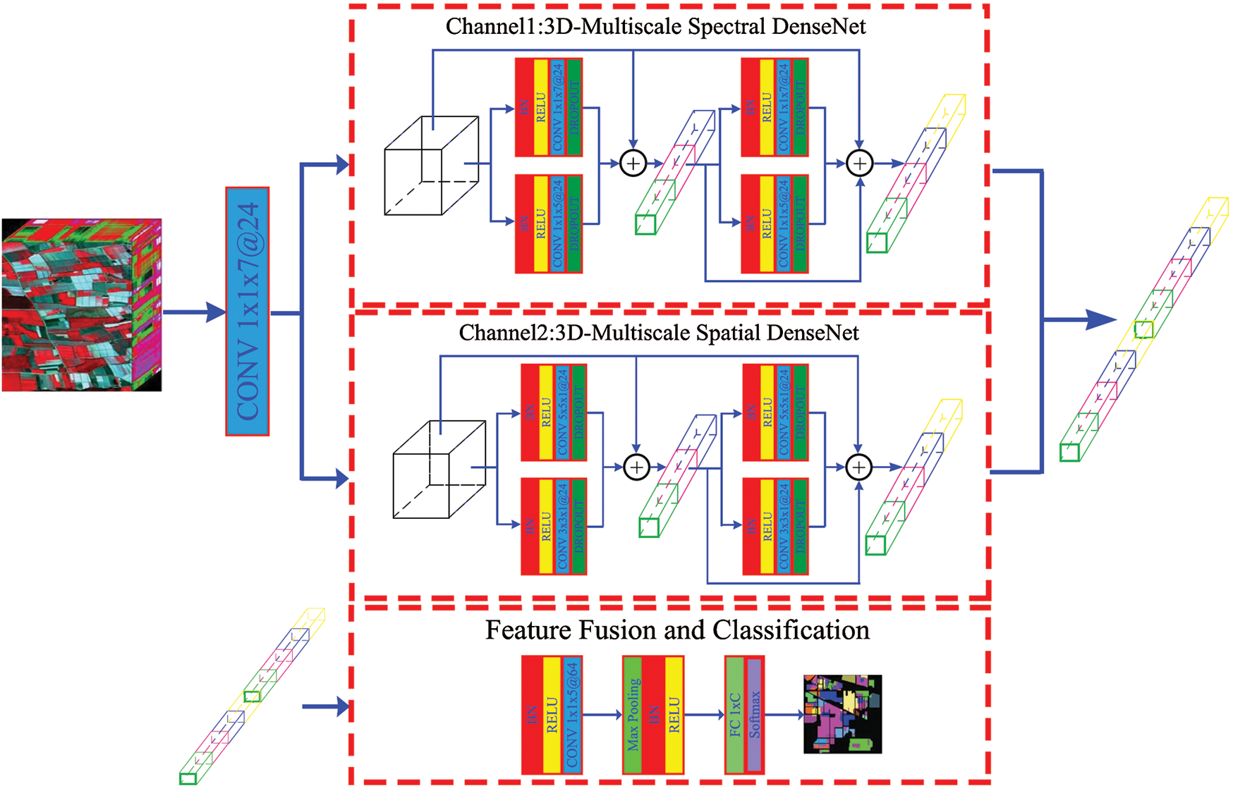
Figure 4: The architecture of 3DMSS
3.3 Channel 1: 3D-Multiscale Spectral DenseNet
3D-Multiscale Spectral DenseNet is shown in Fig. 5. In the training process, for the purpose of dimensionality reduction, the convolution operation is carried out using 24 convolutional kernels with a step size of 2 for the original HSI. The 3D feature map after dimensionality reduction is used as the input to the spectral feature extraction channel.

Figure 5: 3D-Multiscale Spectral DenseNet
In 3D-Multiscale Spectral DenseNet, the multi-scale features of the spectral domain are extracted by using the K convolution kernels with of size p and q, respectively. This is shown in Eqs. (8) and (9):


where  is the input feature map of the 3D-Multiscale Spectral DenseNet.
  is the convolutional operation,
  is the weight of the convolution kernel, and
  is the bias. The superscripts of
  and
and  are the number of convolutional layers and the subscripts are the size of the convolutional kernel.
  is the activation function.
Shallow spectral features at two scales were extracted, and  was obtained by fusing the
  feature maps (a total of
  feature maps) learned at each scale and the original input. This is shown in Eq. (10).

Then,  spectral convolutional kernels of different scales are used to carry out the multi-scale convolution operation on
  , as shown in Eqs. (11) and (12):


where the meanings of each variable are the same as in formula (8) and formula (9). The discriminant spectral feature diagram O will be learned after the extraction of spectral features, as shown in Eq. (13).

3.4 Channel 2: 3D-Multiscale Spatial DenseNet
3D-Multiscale Spatial DenseNet is shown in Fig. 6. In the training process, to achieve the purposes of the dimension reduction, the convolution operation is carried out by using 24 convolutions kernels with a step size of 2 to the original HSI. The 3D feature map after dimension reduction is used as the input data of spatial feature extraction channel.

Figure 6: 3D-Multiscale Spatial DenseNet
In 3D-Multiscale Spatial DenseNet, the multi-scale features of spatial domain are extracted by using the  convolution kernels with sizes of
  and
and  , respectively. As shown in Eqs. (14) and (15):


where,  is the input feature map of the 3D-Multiscale Spectral DenseNet. “
 ” is the convolutional operation.
  is the weight of the convolution kernel.
  is the bias. The superscript of w and b is the number of convolutional layers, and the subscript is the size of the convolutional kernel.
  is the activation function.
The shallow spatial features at two scales were extracted, and the  is obtained by fusing the
  feature maps (a total of
  feature maps) learned at each scale and the original input. As shown in Eq. (16):

Then,  spatial convolution kernels of different scales are used to carry out multi-scale convolution operation on
  , as shown in Eqs. (17) and (18):


The meanings of each variable are the same as formula (14) and formula (15).
The discriminant spectral feature diagram O will be learned after the extraction of spectral features, as shown in Eq. (19):

3.5 Feature Fusion and Classification
As shown in Fig. 7, the results of spectral and spatial learning are concatenated as input followed by a BN, RELU, and convolution layer block, which is the same as the process for Block 2.

Figure 7: Feature fusion and classification
At the end of the block, global average pooling layers are inserted. It was originally designed to replace the traditional FC layer in CNNs. The global average pooling layer contains a much smaller number of parameters than FC layers and can retain good localization ability for a network. It is important to consider two main problems in HSI classification: the overfitting phenomenon caused by the large model scale with limited training data, and the effective extraction of both spectral and spatial features. After the FC layer, a softmax layer is used to obtain the final classification result.
4 Experimental Results and Discussion
We evaluated the performance of the proposed network on three publicly available HSI datasets. First, the main components of 3DMSS are tested, including the number of kernels, the depth of the spectral kernel, the size of the spatial kernel and the number of training samples. Then, the proposed classification model is compared with mainstream approaches in terms of the overall accuracy (OA), average accuracy (AA), and kappa coefficient (K). These are adopted to qualitatively evaluate the classification results.
4.1 Description of the Experimental Data Sets
Three datasets were used: Indian Pines (IN), Kennedy Space Center (KSC), and Salinas (SA). The Indian Pines dataset contains 220 spectral channels and the spatial resolution is 20 m. Each band contains 145 × 145 pixels. The sample size is shown in Tab. 1. The KSC dataset contains 224 spectral channels and 13 land cover categories; the sample size is shown in Tab. 2. The Salinas dataset contains 224 spectral channels, and the spatial resolution is 3.7 m. The sample size is shown in Tab. 3.
Table 1: Indian Pines data sample distribution

Table 2: KSC data sample distribution

Table 3: Indian Pines data sample distribution

4.2 Experimental Setup for the Classification of Labeled Pixels
To set the parameters of 3DMSS, we determined the optimal parameters through a series of experiments, which included the number of convolution kernels, the convolution kernels’ depth of spectral feature channels, the convolution kernels’ size of spatial feature channels, and the number of training samples in each batch.
4.2.1 Effect of the Number of Kernels
This experiment analyzes the effect of the number of convolution kernels on the classification results. For the experimentation, the number of convolution kernels of each residual dense block on Channel 1 and Channel 2 was set to 6, 12, 24, 48, and 64, respectively. The classification accuracy for different numbers of kernels was recorded.
Fig. 8 shows the experimental results. It can be seen that, under certain conditions, increasing the number of convolution kernels can improve the classification accuracy. However, the classification accuracy does not increase linearly with the increase of convolution kernels. With the increase of the number of kernels, the classification accuracy rises first and then flattens out. The experimental results show that the classification accuracy is highest when the number of kernels is 24. It can also be seen that as the number of convolution kernels increases, the computational complexity of the model increases and the time required for classification increases. Therefore, considering the classification accuracy and time complexity, the number of convolution kernels in the convolutional layer is set to 24.
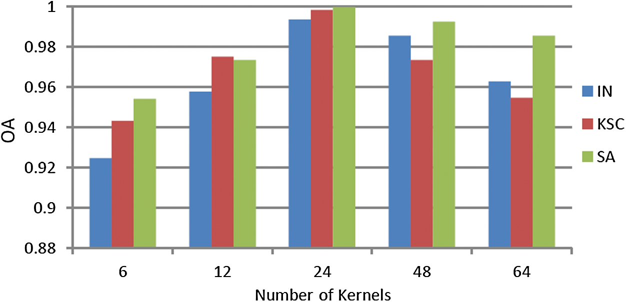
Figure 8: Classification results for each dataset for different kernels
4.2.2 Effect of Different Spectral Kernel Depths
Tab. 4 shows the classification accuracy results for different convolutional kernel depths for 3D-Multiscale Spectral DenseNet. As can be seen from the table, the OA, AA, and Kappa coefficients increased with the increase of convolution kernel depth. As the depth increases  , the accuracy increases slowly or stops increasing. Therefore, the selected convolutional kernel depths for the 3D-Multiscale Spectral DenseNet were
  and
and  .
.
Table 4: OA comparison for different spectral kernel depths

4.2.3 Effect of Different Spatial Kernel Size
Tab. 5 shows the classification accuracy results for different convolutional kernel sizes in 3D-Multiscale Spatial DenseNet. As we can see from the table, the OA, AA, and Kappa coefficients increased with the increase of convolution kernel size. As the size increases  , the accuracy increases slowly or stops increasing. Therefore, convolutional kernel sizes
  and
and  were selected based on the main evaluation indexes.
Table 5: OA comparison for different spatial kernel size

4.3 Classification Results and Discussion
In order to verify the classification performance of 3DMSS proposed in this paper, we compared this with five other classical HSI classification methods on the basis of the OA, AA, and Kappa coefficients. These five methods include: A Support Vector Machine method [6], a Gabor-based method (GABOR) [24], the Image Fusion and Recursive Filtering method [25], 3D-CNN [17], and MS3FE [26]. Tabs. 6–8 show the test results of each method for three datasets. Figs. 9–11 are the visual maps of the different methods on the three datasets.

Figure 9: Experimental results for the different methods for the IN dataset
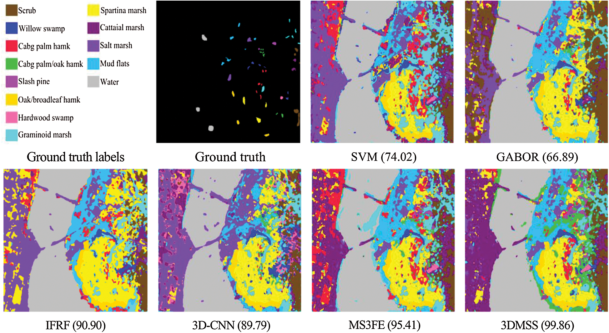
Figure 10: Experimental results for the different methods for the SA dataset

Figure 11: Experimental results for the different methods for the SA dataset
Table 6: Testing of the different methods for the IN dataset

Table 7: Testing of the different methods for the KSC dataset

Table 8: Testing of the different methods for the SA dataset

From Tabs. 6–8, it can be seen that the proposed method attains the best classification performance for the three datasets. The OA for the three datasets is 99.36%, 99.86%, and 99.99%, respectively. Figs. 9–11 are the visual maps of the different methods for the three datasets. It can be seen from the figures that the visual maps for SVM, GABOR, and 3D-CNN have noise and fuzzy classification. The visual maps for RF and MS3FE have clear classification boundaries, but there is still a small amount of noise. The visual maps for 3DMSS are the clearest, and the classification result is the closest to the real object label.
Analyzing the above experimental results, we can draw the following conclusions:
1. The higher the spatial resolution of HSI, the better the classification performance is achieved for the larger convolutional kernel size. The spatial resolution of IN, KSC, and SA is 145 × 145, 512 × 614, and 512 × 217, respectively. Since the resolution of IN is the smallest, IN achieves the best classification accuracy for the convolution kernel size of 3 × 3. The spatial resolution of KSC and SA is greater than IN, so they achieve the best classification accuracy for the slightly larger convolution kernel size 5 × 5.
2. The more spectral bands, the better the classification results for the deeper convolutional kernel. The number of spectral bands for IN, KSC, and SA is 200, 176, and 184, respectively. IN has the most spectral bands, so IN achieves the highest classification accuracy with a convolution kernel depth of 1 × 1 × 7. KSC and SA have fewer spectral bands, so they achieve the highest classification accuracy with a convolution kernel depth of 1 × 1 × 5.
3. Deep learning methods are superior to statistical methods. Among the six compared methods, SVM, Gabor, and RF are traditional classification methods based on statistics. 3D-CNN, MS3FE, and 3DMSS are deep learning methods, and all three use convolutional neural networks. It can be seen from the experimental results that the classification performance for deep learning methods is better than that for statistical methods.
4. Spectral-spatial features help to improve the classification accuracy. Since 3DMSS and MS3FE take into account the spectral-spatial features of HSI, the OA obtained by these two classification methods is significantly higher than that of other methods.
5. The classification results for the residual dense network are better than for other methods. Compared with other classification methods, 3DMSS achieved the best classification results. This is because 3DMSS can extract HSI spectral-spatial features from different scales so that the features of different channels can be shared, and the information flow can be enhanced. At the same time, in order to improve the classification performance, the residual dense block is introduced into 3DMSS to overcome the vanishing gradient problem.
In order to improve the classification performance for HSI, an end-to-end deep 3D-Multiscale Spatial-Spectral DenseNet was proposed in this paper. The work was proposed to handle the problems associated with HSI data such as multiple bands, data redundancy, and limited training samples. The discriminative spectral-spatial features were extracted using 3D-multiscale methods; the features of different blocks can be shared, and the information flow can be enhanced, which solves the problem of the lack of training samples. At the same time, in order to improve the classification performance, residual dense blocks are introduced into 3DMSS to address the vanishing gradient problem. Comparing the classification accuracy with available HSI classification methods for three public HSI datasets, the proposed method shows very promising results, and is highly effective. There is still plenty of scope to develop the proposed method, such as more successful strategies in multi-scale feature fusion and robust classification accuracy for the boundary region. Also, a parallel and distributed fusion strategy, such as in [27,28], will be very helpful in improving the computational efficiency in practice.
Acknowledgement: We thank the anonymous reviewers for their feedback which helped in the improvement of this article.
Funding Statement: The work described in this paper is supported by the National Natural Science Foundation of China (Project No. 11901173), the Heilongjiang Province Natural Science Found (LH2019A030), and the Cultivating Science Foundation of Taizhou University (2019PY014, 2019PY015), the Agricultural Science and Technology Project of Taizhou (20ny13).
Conflicts of Interest: The authors declare that they have no conflicts of interest to report regarding the present study.
1. R. Ji, Y. Gao, R. Hong, Q. Liu, D. Tao et al.. (2014). , “Spectral-spatial constraint hyperspectral image classification,” IEEE Transactions on Geoscience and Remote Sensing, vol. 52, no. 3, pp. 1811–1824. [Google Scholar]
2. V. Menon, S. Prasad and J. E. Fowler. (2015). “Hyperspectral classification using a composite kernel driven by nearest-neighbor spatial features,” in 2015 IEEE International Conference on Image Processing, Milan, Italy, pp. 2100–2104. [Google Scholar]
3. Y. Tarabalka and A. Rana. (2014). “Graph-cut-based model for spectral-spatial classification of hyperspectral images,” in International Geoscience and Remote Sensing Symposium, Quebec, Canada, pp. 3418–3421. [Google Scholar]
4. Y. Tarabalka, M. Fauvel, J. Chanussot and J. A. Benediktsson. (2010). “SVM- and MRF-based method for accurate classification of hyperspectral images,” IEEE Geoscience and Remote Sensing Letters, vol. 7, no. 4, pp. 736–740. [Google Scholar]
5. Y. Wang, W. Yu and Z. Fang. (2020). “Multiple kernel-based SVM classification of hyperspectral images by combining spectral, spatial, and semantic information,” Remote Sensing, vol. 12, no. 1, pp. 120. [Google Scholar]
6. M. Zhang, W. Wang, C. Q. Lu, J. Wang and A. K. Sangaiah. (2019). “Lightweight deep network for traffic sign classification,” Annals of Telecommunications, vol. 75, pp. 369–379. [Google Scholar]
7. W. Wang, Y. Li, T. Zou, X. Wang, J. You et al.. (2020). , “A novel image classification approach via Dense-MobileNet models,” Mobile Information Systems, vol. 2020, pp. 1–8. [Google Scholar]
8. M. Zhang, X. K. Jin, J. Sun, J. Wang and A. K. Sangaiah. (2018). “Spatial and semantic convolutional features for robust visual object tracking,” Multimedia Tools and Applications, vol. 79, no. 21–22, pp. 15095–15115. [Google Scholar]
9. J. Luo, J. H. Qin, X. Y. Xiang, Y. Tan, Q. Liu et al.. (2020). , “Coverless real-time image information hiding based on image block matching and dense convolutional network,” Journal of Real-Time Image Processing, vol. 17, no. 1, pp. 125–135. [Google Scholar]
10. X. Sun, L. F. Shi, C. Y. Yin and J. Wang. (2019). “An improved method in deep packet inspection based on regular expression,” Journal of Supercomputing, vol. 75, no. 6, pp. 3317–3333. [Google Scholar]
11. Y. Yin, H. Y. Wang, X. Yin, R. X. Sun and J. Wang. (2019). “Improved deep packet inspection in data stream detection,” Journal of Supercomputing, vol. 75, no. 8, pp. 4295–4308. [Google Scholar]
12. R. Zhou and B. Tan. (2020). “Electrocardiogram soft computing using hybrid deep learning CNN-ELM,” Applied Soft Computing, vol. 86, pp. 105778. [Google Scholar]
13. P. He, Z. L. Deng, C. Z. Gao, X. N. Wang and J. Li. (2017). “Model approach to grammatical evolution: Deep-structured analyzing of model and representation,” Soft Computing, vol. 21, no. 18, pp. 5413–5423. [Google Scholar]
14. A. Krizhevsky, I. Sutskever and G. E. Hinton. (2017). “ImageNet classification with deep convolutional neural networks,” Communications of the ACM, vol. 60, no. 6, pp. 84–90. [Google Scholar]
15. J. Leng, T. Li, G. Bai, Q. Dong and H. Dong. (2016). “Cube-CNN-SVM: A novel hyperspectral image classification method,” in ICTAI, San Jose, CA, USA, pp. 1027–1034. [Google Scholar]
16. Y. Li, H. Zhang and Q. Shen. (2017). “Spectral-spatial classification of hyperspectral imagery with 3D convolutional neural network,” Remote Sensing, vol. 9, no. 1, pp. 67–78. [Google Scholar]
17. Y. Chen, H. Jiang, C. Li, X. Jia and P. Ghamisi. (2016). “Deep feature extraction and classification of hyperspectral images based on convolutional neural networks,” IEEE Transactions of Geoscience and Remote Sensing, vol. 54, no. 10, pp. 6232–6251. [Google Scholar]
18. S. Wu, S. Zhong and Y. Liu. (2017). “Deep residual learning for image steganalysis,” Multimedia Tools and Applications, vol. 77, no. 9, pp. 10437–10453. [Google Scholar]
19. K. He, X. Zhang, S. Ren and J. Sun. (2016). “Deep residual learning for image recognition,” in IEEE Conference on Computer Vision and Pattern Recognition, Nevada, USA, pp. 770–778. [Google Scholar]
20. G. Huang, Z. Liu, L. Van Der Maaten and K. Q. Weinberger. (2017). “Densely connected convolutional networks,” in IEEE Conference on Computer Vision and Pattern Recognition, Puerto Rico, USA, pp. 2261–2269. [Google Scholar]
21. Z. Xiong, Y. Yuan and Q. Wang. (2018). “AI-Net: Attention inception neural networks for hyperspectral image classification,” in International Geoscience and Remote Sensing Symposium, Valencia, Spain, pp. 2647–2650. [Google Scholar]
22. X. Yang, Y. Ye, X. Li, R. Y. K. Lau, X. Zhang et al.. (2018). , “Hyperspectral image classification with deep learning models,” IEEE Transactions on Geoscience and Remote Sensing, vol. 56, no. 9, pp. 5408–5423. [Google Scholar]
23. Z. Zhong, J. Li, Z. Luo and M. Chapman. (2018). “Spectral–spatial residual network for hyperspectral image classification: A 3-D deep learning framework,” IEEE Transactions on Geoscience and Remote Sensing, vol. 56, no. 2, pp. 847–858. [Google Scholar]
24. L. Z. Huo and P. Tang. (2011). “Spectral and spatial classification of hyperspectral data using SVMs and Gabor textures,” in International Geoscience and Remote Sensing Symposium, Vancouver, BC, Canada, pp. 1708–1711. [Google Scholar]
25. X. Kang, S. Li and J. A. Benediktsson. (2014). “Feature extraction of hyperspectral images with image fusion and recursive filtering,” IEEE Transactions of Geoscience and Remote Sensing, vol. 52, no. 6, pp. 3742–3752. [Google Scholar]
26. L. Jiao, M. Liang, H. Chen, S. Yang, H. Liu et al.. (2017). , “Deep fully convolutional network-based spatial distribution prediction for hyperspectral image classification,” IEEE Transactions on Geoscience and Remote Sensing, vol. 55, no. 10, pp. 5585–5599. [Google Scholar]
27. Z. Wu, Y. Li, A. Plaza, J. Li, F. Xiao et al.. (2016). , “Parallel and distributed dimensionality reduction of hyperspectral data on cloud computing architectures,” IEEE Journal of Selected Topics in Applied Earth Observations and Remote Sensing, vol. 9, no. 6, pp. 2270–2278. [Google Scholar]
28. W. Jing, S. Huo, Q. Miao and X. Chen. (2017). “A model of parallel mosaicking for massive remote sensing images based on spark,” IEEE Access, vol. 5, pp. 18229–18237. [Google Scholar]
 | This work is licensed under a Creative Commons Attribution 4.0 International License, which permits unrestricted use, distribution, and reproduction in any medium, provided the original work is properly cited. |