DOI:10.32604/iasc.2020.013357
| Intelligent Automation & Soft Computing DOI:10.32604/iasc.2020.013357 | |
| Article |
A Novel Semi-Supervised Multi-Label Twin Support Vector Machine
1School of Computer Science and Software Engineering, University of Science and Technology Liaoning, Anshan, 114051, China
2College of Information Science and Engineering, Northeastern University, Shenyang, 110819, China
*Corresponding Author: Qing Ai. Email: lyaiqing@126.com
Received: 04 August 2020; Accepted: 25 September 2020
Abstract: Multi-label learning is a meaningful supervised learning task in which each sample may belong to multiple labels simultaneously. Due to this characteristic, multi-label learning is more complicated and more difficult than multi-class classification learning. The multi-label twin support vector machine (MLTSVM) [1], which is an effective multi-label learning algorithm based on the twin support vector machine (TSVM), has been widely studied because of its good classification performance. To obtain good generalization performance, the MLTSVM often needs a large number of labelled samples. In practical engineering problems, it is very time consuming and difficult to obtain all labels of all samples for multi-label learning problems, so we can only obtain a large number of partially labelled and unlabelled samples and a small number of labelled samples. However, the MLTSVM can use only expensive labelled samples and ignores inexpensive partially labelled and unlabelled samples. Because of the MLTSVM’s disadvantages, we propose an alternative novel semi-supervised multi-label twin support vector machine, named SS-MLTSVM, which can take full advantage of the geometric information of the edge distribution embedded in partially labelled and unlabelled samples by introducing a manifold regularization term into each sub-classifier and use the successive overrelaxation (SOR) method to speed up the solving process. Experimental results on several publicly available benchmark multi-label datasets show that, compared with the classical MLTSVM, our proposed SS-MLTSVM has better classification performance.
Keywords: Multi-label learning; semi-supervised learning; TSVM; MLTSVM
Multi-label learning is a meaningful supervised learning task, wherein each sample may belong to multiple different labels simultaneously. In real life, many applications employ multi-label learning, including text classification [2,3], image annotation [4], bioinformatics [5], and so on [6]. Because the samples can have multiple labels simultaneously, multi-label learning is more complicated and more difficult than multi-class classification learning. At present, there are two kinds of methods to solve multi-label learning problems: problem transformation and algorithm adaptation. The problem transformation solves the multi-label learning problem by transforming it into one or more single-label problems, such as binary relevance (BR) [7], classifier chains (CC) [8], label powerset (LP) [9], calibrated label ranking (CLR) [10], and random k-labelsets (RAKEL) [11]. The algorithm adaptation extends the existing single-label learning algorithm to handle multi-label learning problems, such as multi-label k-nearest neighbour (ML-kNN) [12], multi-label decision tree (ML-DT) [13], ranking support vector machine (Rank-SVM) [14], and collective multi-label classifier (CML) [15].
The TSVM [16], proposed by Jayadeva, is used to solve classification problems. It has been widely studied because of its good classification performance. Subsequent to its release, many improved algorithms have been proposed [17–29]. The aforementioned improved algorithms can solve only single-label learning problems, not multi-label learning problems. In 2016, Chen et al. extended the TSVM to solve multi-label learning problems and proposed a multi-label twin support vector machine (MLTSVM) [1]. Compared with other traditional multi-label classification algorithms, the MLTSVM has better generalization performance. Thereafter, many improved algorithms of MLTSVM have been proposed [30,31]. Hanifelou et al. introduced local information and structural information of samples into the MLTSVM and proposed the k-nearest neighbour-based MLTSVM with priority of labels (PKNN-MLTSVM) [30]. Meisam et al. proposed the structural least square twin support vector machine for multi-label learning (ML-SLSTSVM) [31], which proposed a least squares version of the MLTSVM and added structural information of samples.
The aforementioned improvements to the MLTSVM mainly focused on improving the generalization performance and learning speed. It is very time consuming and difficult to obtain all labels of all samples for multi-label learning problems; in fact, we can obtain only a large number of partially labelled and unlabelled samples and a small number of labelled samples. However, the MLTSVM and its improvements can use only expensive labelled samples and ignores inexpensive partially labelled and unlabelled samples. Because of this disadvantage, we propose a novel semi-supervised MLTSVM, named SS-MLTSVM, which can take full advantage of the geometric information of the edge distribution embedded in partially labelled and unlabelled samples by introducing a manifold regularization term into each sub-classifier and use the successive overrelaxation (SOR) method to increase the solving speed. Experimental results show that, compared with the MLTSVM, our SS-MLTSVM has better classification performance.
The structure of this paper is as follows: Section 2 introduces some related works, such as the TSVM and MLTSVM. In Section 3, the SS-MLTSVM is introduced in detail, including the linear model, nonlinear model, decision rules and training algorithm. The fourth section gives the experimental results of the proposed algorithm on the benchmark datasets. The fifth section is the conclusion.
For the binary classification problem, we suppose the training set is  , where
  is the training sample and
  is the label corresponding to the training sample
  . We denote positive training samples by
  and negative training samples by
  .
.  is the total number of training samples.
The TSVM is aimed to find two nonparallel hyperplanes:

The original problem of TSVM is:
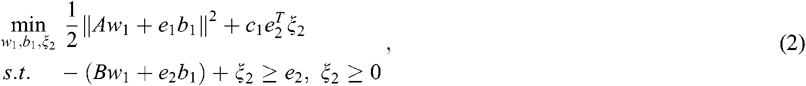
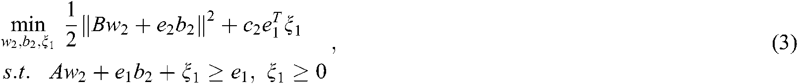
where  and
and  are the penalty parameters,
  and
and  are the slack variables, and
  and
and  are all 1 vector of the proper dimension.
By introducing the Lagrange multiplier, the dual problems of (2) and (3) can be obtained as follows:

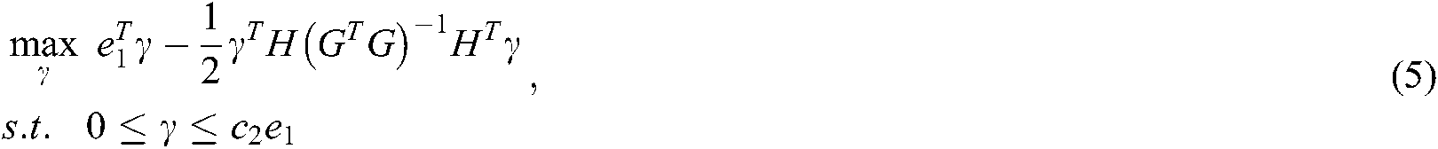
where 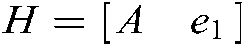 ,
,  , and
, and  and
and  are the Lagrange multipliers.
The two hyperplanes can be obtained by solving the dual problems as follows:


For the multi-label problem, we denote the training set as:

where  is the training sample,
  is the label set of the sample
  ,
,  (
( ),
),  is the total number of training samples and
  is the total number of labels.
The MLTSVM seeks  hyperplanes:

We denote the samples belonging to the kth class by  and the other samples by
  . The original problem for label k is:
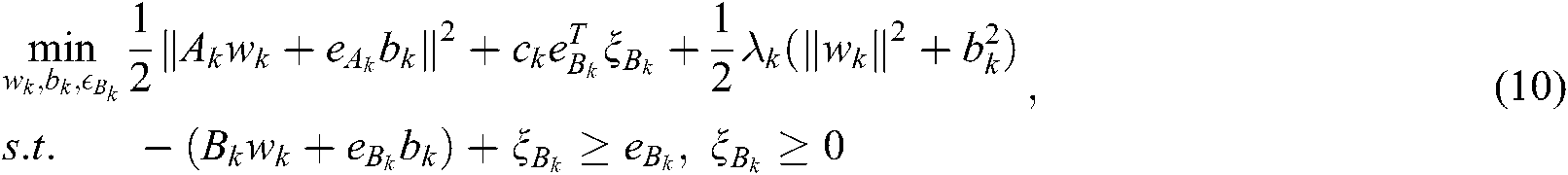
where  and
and  are the penalty parameters,
  and
and  are all 1 vector of the proper dimension, and
  is the slack variable.
By introducing the Lagrange multiplier, the dual problems of (10) can be obtained as follows:
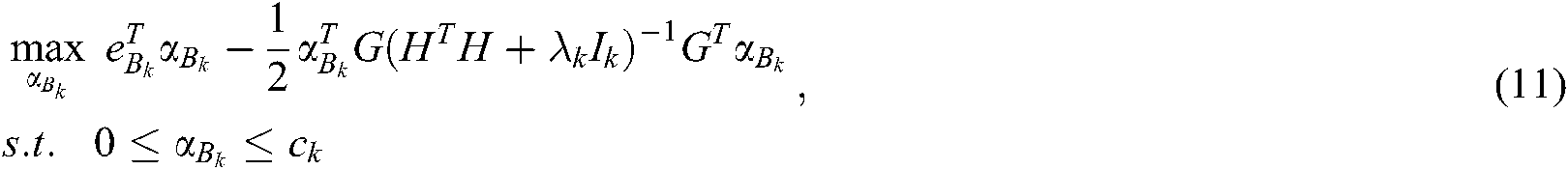
where  ,
,  ,
,  are the diagonal matrices of the proper dimension, and
  is the Lagrange multiplier.
By solving the dual problem (11), we can obtain:

Similar to the MLTSVM, the ML-STSVM also seeks  hyperplanes:

The original problem for label k is:
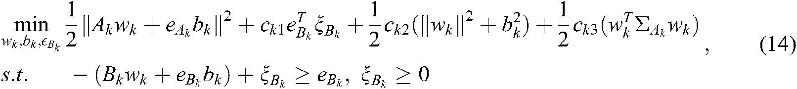
where  are the penalty parameters,
  is the slack factor,
  and
and  are all 1 vector of the proper dimension, and
  ,
,  is the covariance matrix of the ith cluster in
  .
.
The dual problem of (14) is:
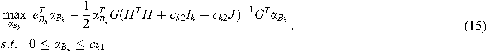
where  ,
,  , and
, and  .
.  are the diagonal matrices of the proper dimension, and
  is the Lagrange multiplier.
By solving the dual problem (15), we can obtain:

For the semi-supervised multi-label problem, we define the training set as follows:

where  is the training sample and
  is the label matrix of the sample
  .
.
3.1 Manifold Regularization Framework
The manifold regularization framework [32], proposed by Belkin et al., can effectively solve semi-supervised learning problems. The objective optimization function of the manifold regularization framework can be expressed as follows:

where  is the decision function to be solved,
  is the loss function on the labelled samples, the regularization term
  is used to control the complexity of the classifier, and the manifold regularization term
  reflects the internal manifold structure of the data distribution.
Similar to the MLTSVM, for each label, the SS-MLTSVM seeks a hyperplane:

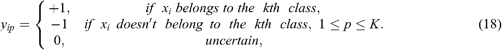
For the kth label, we denote the samples that definitely belong to the kth class by  , i.e.,
  ; the samples that definitely do not belong to the kth class by, i.e.,
  ; and the samples that are uncertain of belonging to the kth class, by
  , i.e.,
  ;
;  .
.
To make full use of  , according to the manifold regularization framework, in our SS-MLTSVM, the loss function
  is replaced by a square loss function and a Hinge loss function, namely:

The regularization term  can be replaced by:

The manifold regularization term  can be expressed as:

where  .
.  is the Laplace matrix, where
  is defined as follows:

and  is defined as follows:

For the kth label, the original problem in the linear SS-MLTSVM is:
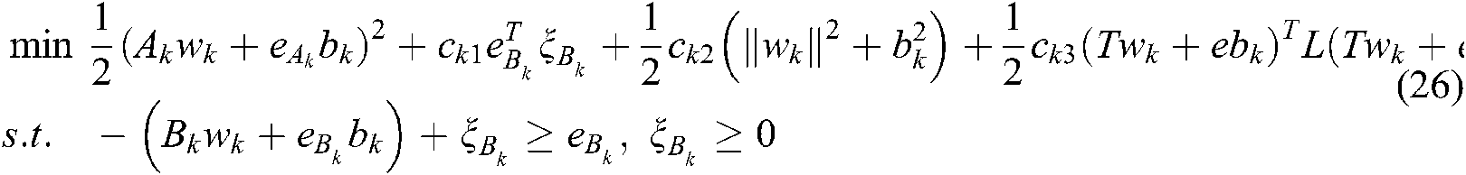
where  are the penalty parameters,
  is the slack factor,
  ,
,  and
and  are all 1 vector of the proper dimension, and
  is the Laplace matrix.
The Lagrange function of (26) is as follows:
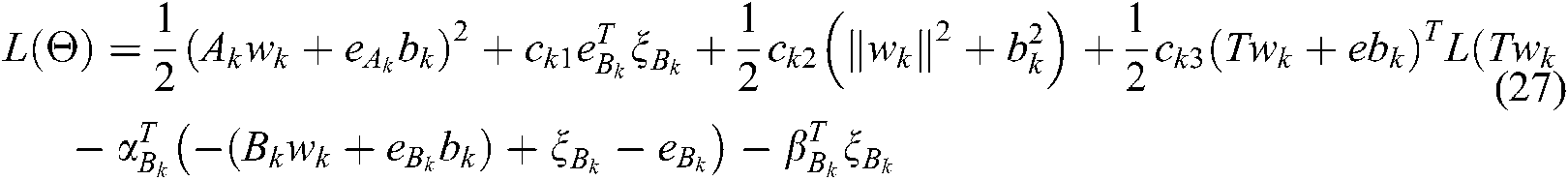
where  .
.  and
and  are Lagrange multipliers. Using KKT theory, we can obtain:


According to (28)–(30), we can obtain the dual problem of (26) as follows:
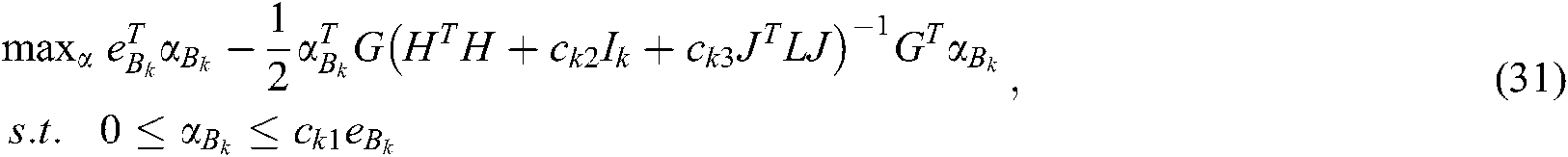
where  ,
,  , and
, and  .
.
For the kth label, the hyperplane can be obtained by solving the dual problem as follows:

In this section, using the kernel-generated surfaces, we extend the linear SS-MLTSVM to the nonlinear case. For each label, the nonlinear SS-MLTSVM seeks the following hyperplanes:

where  is a kernel function. Similar to the linear case, the regularization term
  and the manifold regularization term
  in (19) can be, respectively, expressed as:


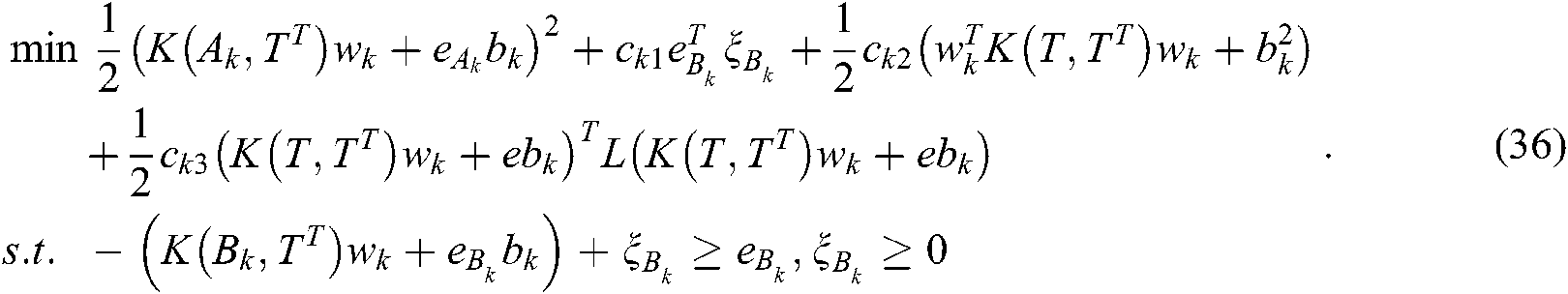
The original problem of the nonlinear SS-MLTSVM is as follows:
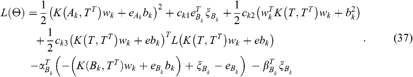
The Lagrange function of (36) is as follows:
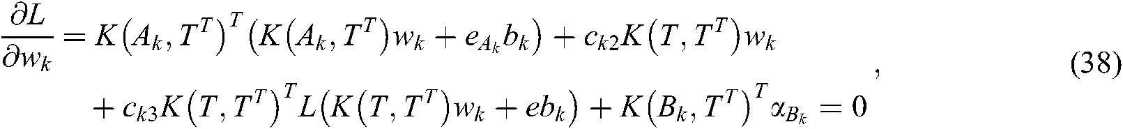
According to KKT theory, we can obtain:


According to (38)–(40), we can obtain the dual problem of (32) as follows:
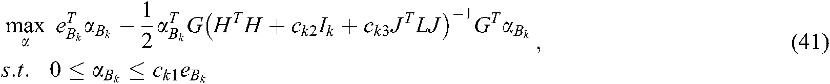
where  ,
,  ,
,  and
and  .
.
By solving the dual problem, the hyperplane of the kth label can be obtained as follows:

In this subsection, we present the decision function of our SS-MLTSVM. For a new sample  , as mentioned above, if the sample
  is proximal enough to a hyperplane, it can be assigned to the corresponding class. In other words, if the distance
  between
  and the kth hyperplane

is less than or equal to the given value  ,
,  , then the sample
  is assigned to the kth class. To choose the proper
  , we apply the strategy in the MLTSVM, which is a simple and effective method, i.e., we set
 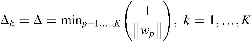 .
.
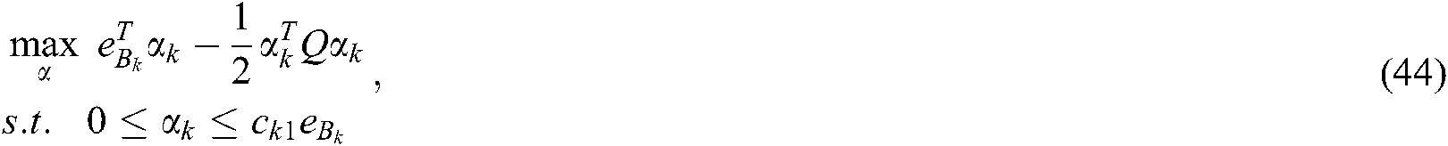
In this subsection, we use SOR to solve the dual problems (31) and (41) efficiently [33]. For convenience, we set  . The dual problems (31) and (41) can be uniformly rewritten as:
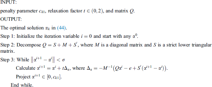
Algorithm 1 only updates one variable  in each iteration, which can effectively reduce the complexity of the algorithm and speed up the learning process.
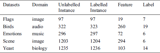
In this section, we present the classification results of backpropagation for multi-label learning (BPMLL) [34], ML-kNN, Rank-SVM, MLTSVM and our SS-MLTSVM on the benchmark datasets. All the algorithms are implemented in MATLAB (R2017b), and the experimental environment is an Intel Core i3 processor and 4G RAM. In the experiments, we use five common datasets for multi-label learning, including flags, birds, emotions, yeast and scene (see Tab. 1). To verify the classification performance of our SS-MLTSVM, we choose 50% of the dataset as labelled samples and the remaining samples as unlabelled samples.
Table 1: Detailed description of the datasets
The parameters of the algorithm have an important impact on the classification performance. We use 10-fold cross-validation to select the appropriate parameters for each algorithm. For BPMLL, the number of hidden neurons is set to 20% of the input dimension, and the number of training epochs is 100. For the ML-kNN, the number of nearest neighbours is set to 5. For the Rank-SVM, the penalty parameter  is selected from
 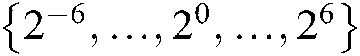 . For the MLTSVM, we select penalty parameters
 and
and  from
from  . For the SS-MLTSVM, we select penalty parameters
  ,
,  , and
, and  from
from 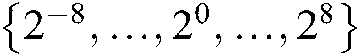 .
.
In the experiments, we use five popular metrics to evaluate the multi-label classifiers, which are Hamming loss, average precision, coverage, one_error and ranking loss. Next, we introduce these five evaluation metrics in detail.
We denote the total number of samples by  and the total number of labels by
  .
.  and
and  represent the relevant label set and irrelevant label set of sample
  , respectively. The function
  returns a confidence of
  being the right label of sample
  , and the function
  returns a descending rank of
  for any
  .
.
The evaluation criteria are used to measure the proportion of labels that are wrongly classified.

where  is the predicted label set of sample
  .
.
The evaluation criteria are used to measure how many steps we need to go down the ranked label list to contain all true labels of a sample.

The evaluation criteria are used to measure the proportion of samples whose label with the highest prediction probability is not in the true label set.

where

The evaluation criteria are used to measure the proportion of label pairs that are ordered reversely.

The evaluation criteria are used to measure the proportion of labels ranked above a particular label  .
.

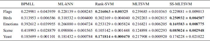
We show the average precision, coverage, Hamming loss, one_error and ranking loss of each algorithm on the benchmark datasets in Tabs. 2–6. From Tabs. 2 and 3, we can observe that, for average precision and coverage, our SS-MLTSVM is superior to the other algorithms for each dataset, while for Hamming loss, one_error and ranking loss, no algorithm is superior to any other algorithm on all datasets. Therefore, for Hamming loss, one_error and ranking loss, we proceed to use the Friedman test to evaluate each algorithm statistically. The Friedman statistics is as follows:
Table 2: Average precision of algorithms on the benchmark datasets
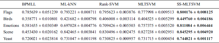
Table 3: Coverage of algorithms on the benchmark datasets
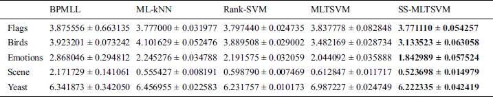
Table 4: Hamming loss of algorithms on the benchmark datasets
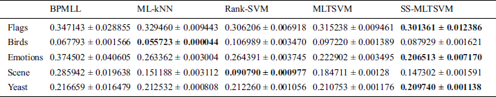
Table 5: One_error of algorithms on the benchmark datasets
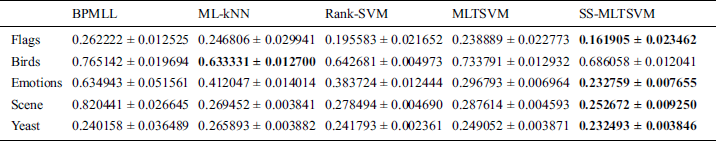
Table 6: Ranking loss of algorithms on the benchmark datasets

where  ,
,  represents the rank of the jth algorithm on the ith dataset. Because
  is undesirably conservative, we apply the better statistic

where  is the number of algorithms and
  is the number of datasets.
We can obtain  ,
,  ,
,  , and
, and  ,
,  ,
,  . When the significance level is
  ,
,  . Because
  ,
,  and
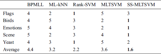
and  are larger than the critical values, 5 algorithms have significant differences for the three metrics. We list the rank of the different algorithms in light of Hamming loss, one_error and ranking loss in Tabs. 7–9. From Tabs. 7–9, we can see that the average rank of our SS-MLTSVM is better than other algorithms; thus, the SS-MLTSVM has better classification performance.
Table 7: Ranks of algorithms in light of Hamming loss
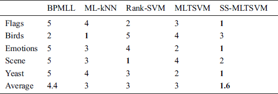
Table 8: Ranks of algorithms in light of one_error
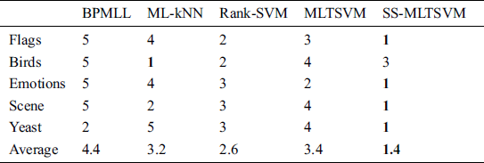
Table 9: Ranks of algorithms in light of ranking loss
From the above analysis, we can conclude that our SS-MLTSVM is superior to the other algorithms for all metrics.
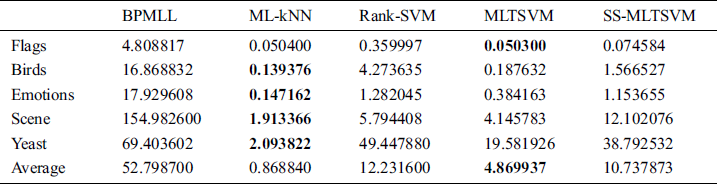
We show the learning time of different algorithms on the benchmark datasets in Tab. 10. From Tab. 10, we can observe that our SS-MLTSVM has a lower learning speed than the MLTSVM. This is mainly because our SS-MLTSVM adds a manifold regularization term that needs to solve the Laplace matrix with whole samples. Even so, our SS-MLTSVM still has great advantages compared with the Rank-SVM and BPMLL.
Table 10: Learning time of algorithms on the benchmark datasets
In this subsection, we investigate the effect of the size of unlabelled samples on the classification performance. In Figs. 1–5, we show the classification performance of our SS-MLTSVM and the MLTSVM on different datasets for different sizes of unlabelled samples.
Figure 1: Average precision of the SS-MLTSVM and MLTSVM for unlabelled samples of different sizes
Figure 2: Hamming loss of the SS-MLTSVM and MLTSVM for unlabelled samples of different sizes
Figure 3: One_error of the SS-MLTSVM and MLTSVM for unlabelled samples of different sizes
Figure 4: Ranking loss of the SS-MLTSVM and MLTSVM for unlabelled samples of different sizes
Figure 5: Coverage of the SS-MLTSVM and MLTSVM for unlabelled samples of different sizes
From Figs. 1–5, we can observe that the classification performance of the SS-MLTSVM is better than that of the MLTSVM in all cases. With the increase of unlabelled samples, the advantages of the SS-MLTSVM become increasingly obvious, because, with the increase of in unlabelled samples, the SS-MLTSVM can make full use of the embedded geometric information, construct a more reasonable classifier, and further improve the classification performance.
In this paper, a novel SS-MLTSVM is proposed to solve semi-supervised multi-label classification problems. By introducing the manifold regularization term into the MLTSVM, we construct a more reasonable classifier and use SOR to speed up learning. Theoretical analysis and experimental results show that, compared with the existing multi-label classifiers, the SS-MLTSVM can take full advantage of the geometric information embedded in partially labelled and unlabelled samples and effectively solve semi-supervised multi-label classification problems. It should be pointed out that our SS-MLTSVM does not consider the correlation among labels; however, the correlation among labels is very valuable to improve the generalization performance. Therefore, more effective methods of obtaining correlation among labels should be addressed in the future.
Funding Statement: This research was funded in part by the Natural Science Foundation of Liaoning Province in China (2020-MS-281, 20180551048, 20170520248) and in part by the Talent Cultivation Project of the University of Science and Technology Liaoning in China (2018RC05).
Conflicts of Interest: The authors declare that they have no conflicts of interest to report regarding the present study.
1. W. J. Chen, Y. H. Shao and C. N. Li. (2016). “MLTSVM: A novel twin support vector machine to multi-label learning,” Pattern Recognition, vol. 52, pp. 61–74, . DOI 10.1016/j.patcog.2015.10.008. [Google Scholar]
2. H. Peng, J. Li and S. Wang, “Hierarchical taxonomy-aware and attentional graph capsule RCNNs for large-scale multi-label text classification,” IEEE Transactions on Knowledge and Data Engineering, to be published. [Google Scholar]
3. T. Wang, L. Liu and N. Liu. (2020). “A multi-label text classification method via dynamic semantic representation model and deep neural network,” Applied Intelligence, vol. 50, no. 8, pp. 2339–2351, . DOI 10.1007/s10489-020-01680-w. [Google Scholar]
4. Y. Liu, K. Wen and Q. Gao. (2018). “SVM based multi-label learning with missing labels for image annotation,” Pattern Recognition, vol. 78, pp. 307–317, . DOI 10.1016/j.patcog.2018.01.022. [Google Scholar]
5. Y. Guo, F. Chung and G. Li. (2019). “Multi-label bioinformatics data classification with ensemble embedded feature selection,” IEEE Access, vol. 7, pp. 103863–103875, . DOI 10.1109/ACCESS.2019.2931035. [Google Scholar]
6. K. Yang, C. She, W. Zhang, J. Yao and S. Long. (2019). “Multi-label learning based on transfer learning and label correlation,” Computers, Materials & Continua, vol. 61, no. 1, pp. 155–169, . DOI 10.32604/cmc.2019.05901. [Google Scholar]
7. M. R. Boutell, J. Luo, X. Shen and C. M. Brown. (2004). “Learning multi-label scene classification,” Pattern Recognition, vol. 37, no. 9, pp. 1757–1771, . DOI 10.1016/j.patcog.2004.03.009. [Google Scholar]
8. J. Read, B. Pfahringer, G. Holmes and E. Frank. (2011). “Classifier chains for multi-label classification,” Machine Learning, vol. 85, no. 3, pp. 333–359, . DOI 10.1007/s10994-011-5256-5. [Google Scholar]
9. E. A. Cherman, M. C. Monard and J. Metz. (2011). “Multi-label problem transformation methods: A case study,” CLEI Electronic Journal, vol. 14, no. 1, pp. 1–10. [Google Scholar]
10. J. Fürnkranz, E. Hüllermeier, E. L. Mencía and K. Brinker. (2008). “Multi-label classification via calibrated label ranking,” Machine Learning, vol. 73, no. 2, pp. 133–153, . DOI 10.1007/s10994-008-5064-8. [Google Scholar]
11. G. Tsoumakas and I. Vlahavas. (2007). “Random k-labelsets: An ensemble method for multilabel classification,” in Proc. of the 18th European Conf. on Machine Learning (ECML 2007Warsaw, Poland, pp. 406–417. [Google Scholar]
12. M. L. Zhang and Z. H. Zhou. (2007). “ML-KNN: A lazy learning approach to multi-label learning,” Pattern Recognition, vol. 40, no. 7, pp. 2038–2048, . DOI 10.1016/j.patcog.2006.12.019. [Google Scholar]
13. A. Clare and R. D. King. (2001). “Knowledge discovery in multi-label phenotype data, ” in European Conf. on Principles of Data Mining and Knowledge Discovery (PKDD 2001). Freiburg, Germany, 42–53. [Google Scholar]
14. A. Elisseeff and J. Weston. (2001). “A kernel method for multi-labelled classification,” Advances in Neural Information Processing Systems, vol. 14, pp. 681–687. [Google Scholar]
15. N. Ghamrawi and A. McCallum. (2005). “Collective multi-label classification, ” in Int. Conf. on Information and Knowledge Management (ACM CIKM 2005). Bremen, Germany, 195–200. [Google Scholar]
16. Jayadeva, R. Khemchandani and S. Chandra. (2007). “Twin support vector machines for pattern classification,” IEEE Transactions on Pattern Analysis and Machine Intelligence, vol. 29, no. 5, pp. 905–910, . DOI 10.1109/TPAMI.2007.1068. [Google Scholar]
17. H. Wang and Z. Zhou. (2017). “An improved rough margin-based v-twin bounded support vector machine,” Knowledge-Based Systems, vol. 128, no. 15, pp. 125–138, . DOI 10.1016/j.knosys.2017.05.004. [Google Scholar]
18. A. Mir and J. A. Nasiri. (2018). “KNN-based least squares twin support vector machine for pattern classification,” Applied Intelligence, vol. 48, no. 12, pp. 4551–4564, . DOI 10.1007/s10489-018-1225-z. [Google Scholar]
19. X. Peng. (2010). “A ν-twin support vector machine (ν-TSVM) classifier and its geometric algorithms,” Information Sciences, vol. 180, no. 20, pp. 3863–3875, . DOI 10.1016/j.ins.2010.06.039. [Google Scholar]
20. X. Chen, J. Yang and Q. Ye. (2011). “Recursive projection twin support vector machine via within-class variance minimization,” Pattern Recognition, vol. 44, no. 10–11, pp. 2643–2655, . DOI 10.1016/j.patcog.2011.03.001. [Google Scholar]
21. Q. Ai, A. Wang, Y. Wang and H. Sun. (2019). “An improved Twin-KSVC with its applications,” Neural Computing and Applications, vol. 31, no. 10, pp. 6615–6624, . DOI 10.1007/s00521-018-3487-0. [Google Scholar]
22. F. Xie and Y. Xu. (2019). “An efficient regularized K-nearest neighbor structural twin support vector machine,” Applied Intelligence, vol. 49, no. 12, pp. 4258–4275, . DOI 10.1007/s10489-019-01505-5. [Google Scholar]
23. Z. Qi, Y. Tian and Y. Shi. (2012). “Laplacian twin support vector machine for semi-supervised classification,” Neural Networks, vol. 35, pp. 46–53, . DOI 10.1016/j.neunet.2012.07.011. [Google Scholar]
24. J. Xie, K. Hone, W. Xie, X. Gao, Y. Shi et al. (2013). , “Extending twin support vector machine classifier for multi-category classification problems,” Intelligent Data Analysis, vol. 17, no. 4, pp. 649–664, . DOI 10.3233/IDA-130598. [Google Scholar]
25. H. Gu. (2014). “A directed acyclic graph algorithm for multi-class classification based on twin support vector machine,” Journal of Information and Computational Science, vol. 11, no. 18, pp. 6529–6536, . DOI 10.12733/jics20105038. [Google Scholar]
26. Y. Xu, R. Guo and L. Wang. (2013). “A twin multi-class classification support vector machine,” Cognitive Computation, vol. 5, no. 4, pp. 580–588, . DOI 10.1007/s12559-012-9179-7. [Google Scholar]
27. C. Angulo, X. Parra and C. Andreu. (2003). “K-SVCR: A support vector machine for multi-class classification,” Neurocomputing, vol. 55, no. 1–2, pp. 57–77, . DOI 10.1016/S0925-2312(03)00435-1. [Google Scholar]
28. Z. X. Yang, Y. H. Shao and X. S. Zhang. (2013). “Multiple birth support vector machine for multi-class classification,” Neural Computing and Applications, vol. 22, no. S1, pp. 153–161, . DOI 10.1007/s00521-012-1108-x. [Google Scholar]
29. Q. Ai, A. Wang, Y. Wang and H. Sun. (2018). “Improvements on twin-hypersphere support vector machine using local density information,” Progress in Artificial Intelligence, vol. 7, no. 3, pp. 167–175, . DOI 10.1007/s13748-018-0141-0. [Google Scholar]
30. Z. Hanifelou, P. Adibi and S. A. Monadjemi. (2018). “KNN-based multi-label twin support vector machine with priority of labels,” Neurocomputing, vol. 322, pp. 177–186, . DOI 10.1016/j.neucom.2018.09.044. [Google Scholar]
31. M. AzadManjiri, A. Amiri and S. A. Saleh. (2020). “ML-SLSTSVM: A new structural least square twin support vector machine for multi-label learning,” Pattern Analysis and Applications, vol. 23, no. 1, pp. 295–308, . DOI 10.1007/s10044-019-00779-2. [Google Scholar]
32. M. Belkin, P. Niyogi and V. Sindhwani. (2006). “Manifold regularization: A geometric framework for learning from labeled and unlabeled examples,” Journal of Machine Learning Research, vol. 7, pp. 2399–2434. [Google Scholar]
33. O. L. Mangasarian and D. R. Musicant. (1999). “Successive overrelaxation for support vector machines,” IEEE Transactions on Neural Networks, vol. 10, no. 5, pp. 1032–1037, . DOI 10.1109/72.788643. [Google Scholar]
34. M. L. Zhang and Z. H. Zhou. (2006). “Multilabel neural networks with applications to functional genomics and text categorization,” IEEE Transactions on Knowledge and Data Engineering, vol. 18, no. 10, pp. 1338–1351, . DOI 10.1109/TKDE.2006.162. [Google Scholar]
 | This work is licensed under a Creative Commons Attribution 4.0 International License, which permits unrestricted use, distribution, and reproduction in any medium, provided the original work is properly cited. |