DOI:10.32604/iasc.2021.014152
| Intelligent Automation & Soft Computing DOI:10.32604/iasc.2021.014152 | |
| Article |
Study of Sugarcane Buds Classification Based on Convolutional Neural Networks
1Hechi University, Yizhou, 546300, China
2Guangxi Normal University, Guilin, 541004, China
3JPMorgan Chase & Co. 270 Park Avenue, New York,10017, USA
*Corresponding Author: Jiansheng Peng. Email:sheng120410@163.com
Received: 02 September 2020; Accepted: 30 October 2020
Abstract: Accurate identification of sugarcane buds, as one of the key technologies in sugarcane plantation, becomes very necessary for its mechanized and intelligent advancements. In the traditional methods of sugarcane bud recognition, a significant amount of algorithms work goes into the location and recognition of sugarcane bud images. A Convolutional Neural Network (CNN) for classifying the bud conditions is proposed in this paper. Firstly, we convert the colorful sugarcane images into gray ones, unify the size of them, and make a TFRecord format data set, which contains 1100 positive samples and 1100 negative samples. Then, a CNN mode is developed to classify the buds into good ones or bad ones. This model contains two convolutional layers and two pooling layers, which go into two full connected layers at the end. The bud dataset is divided into three sets: training set (80%), validation set (10%) and test set (10%). After the repeated training, the structure and parameters of the model are optimized, and an optimal application model is obtained. The experiment results demonstrate that the recognition accuracy of sugarcane bud reaches to 99%, which is about 6% higher than traditional methods. It proves that the CNN model is feasible to classify sugarcane buds.
Keywords: Sugarcane bud; classification; convolutional neural networks
Sugarcane is widely planted in China. According to the “China Statistical Yearbook-2019”, the area of sugarcane planted is 1,406,000 hectares. As we know that China is a big agricultural country, but the agricultural industry is backward relatively. Artificial sugarcane planting suffers from low productivity and poor economic benefits. In the process of sugarcane harvesting, transportation, seed retention and cutting, the buds are easily damaged. Therefore, the identification of the conditions of sugarcane buds becomes the key factor in the automatic sugarcane planting. And the intact seed buds of sugarcane are the basic guarantee for the budding rate of new ones. So, it is necessary to discriminate the good buds from the bad ones, such as buds dropping, dead buds, rotten buds [1,2].
Many researches are made to detect the sugarcane nodes [3–7], but few attempt to judge the conditions of the sugarcane buds. They use the sugarcane nodes to determine indirectly the position of the sugarcane buds. Then the cutter is controlled to avoid bud damage during sugarcane cutting. Although these methods have limited the average rate of damaged buds within 2%, it is impossible to detect damaged buds before sugarcane cutting. Thus, it will greatly influence the production and the economic benefit of sugarcane. Lu [4] proposes an improved 8-points equivalent maximum inscribed circle method to separate and locate the sugarcane buds. He uses image processing technology to segment the bud based on its color and shape features. But this method generalizes not well. Huang et al. [8] propose a machine learning based method to classify the integrity of sugarcane buds. This method uses Bayesian decision model to detect whether the buds are defective or damaged. However, it needs to manually extract five classification features including the minimum gray value, the maximum gray value, the mean gray value, the standard deviation of gray value, and the gray scale median from the effective sugarcane bud area. It is undeniable fact that there are many defects in these methods. The biggest problem is that the extraction of the seed buds’ characteristics has to be spotted artificially before recognition. The extraction algorithm is more complicated and the workload is heavy.
Deep learning has been widely used in image recognition and classification [9–18]. Inspired by the LeNet-5 model [19], we propose a CNN-based network model to classify the sugarcane bud conditions which reduce the work of extracting artificial seed bud features in the early stage, and improve the recognition rate. Our method mainly has two steps. The first step is to pre-process the bud images. It is to convert the color image of sugarcane into a gray one and unify the size of the image to create a data set in TFRecord format. The second step is to design and train the CNN mode. The bud data set is divided into three groups: 80% is used as the training set, 10% is used as the validation set, and 10% is used as the test set. Through the repetition training, the structure and parameters of the model are optimized. And the best application model is finally obtained which improves the recognition rate.
2 Pretreatment of Sugarcane Bud Image Data
TFRecord data file is a binary file that stores any data form by converting them into the TensorFlow form, and make the datasets of TensorFlow matching the network applications more easily. It is convenient to copy and call in training data loading as well. Converting sugarcane image data into TFRecord data sets cannot only call image data model training more quickly, but also reduce the time needed to load image data set and train section during model training. Therefore, it is necessary to encapsulate sugarcane image data set with TFRecord data set.
To make TFRcord data set, we first select 1100 bad sugarcane buds and 1100 good ones from the collected images, and then save them in the designated path respectively. The format naming is shown in Fig. 1.
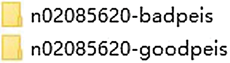
Figure 1: Naming of sugarcane bud
The good and bad sugarcane bud images are shown in Figs. 2 and 3 respectively. It is not difficult to see from the image that the biological structure of the intact seed bud is complete, and the surface or internal biological structure of the damaged seed bud is damaged and cannot germinate normally as well.
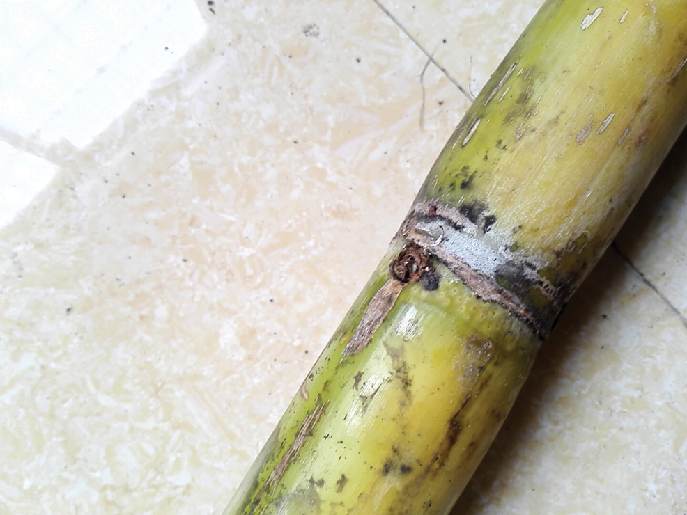
Figure 2: Bad sugarcane bud
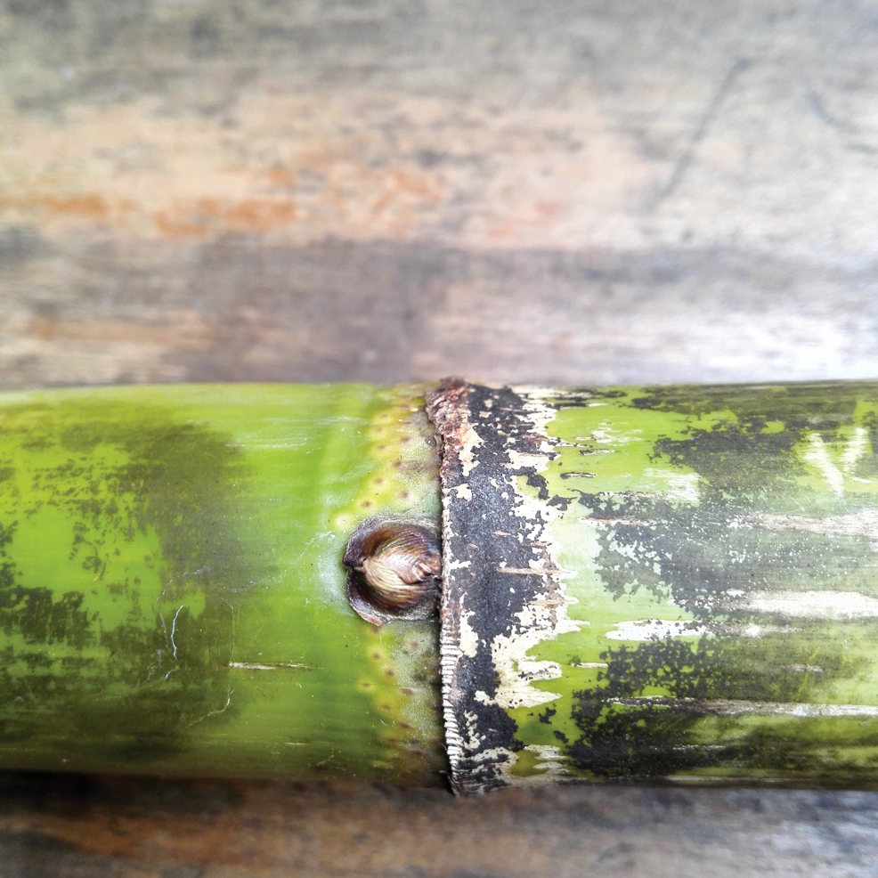
Figure 3: Good sugarcane bud
However, the original images mentioned above cannot be used directly for training. Since most of the original images have different sizes, they need to be unified in size first of all. When performing model is training, corresponding labels should be marked in the image file. The system changes the color space into gray when converting the image data format. And the image size is modified to a same size: 250 pt × 151 pt, and a two-dimensional image label is attached to each image. The entire data set is divided into 80% training set, 10% validation set and 10% test set.
3 Construction of Sugarcane Bud Recognition Model
3.1 Convolutional Neural Networks
Convolutional neural networks (CNN) reduce the complexity of the model by the weight sharing which is very popular in the field of image and speech recognition. The CNN-based model performs outstanding in multi-dimensional data inputting field. It has good robustness in translation, rotation and scaling image. Image recognition based on CNN has more advantages. Compared with the traditional network structure, the biggest advantage of CNN is the two special design methods: convolutional layer and pooling layer. The convolutional neural network is connected to the upper layer by local connections and weight sharing which greatly reduces the number of model parameters. Because of this special design, the original image can be sent to CNN without the special complicated processing.
The most typical network structure is LeNet-5, which can be used in image recognition. LeNet-5 has a basic convolutional neural network modules: convolutional layer, pooling layer and fully connected layer. It is a model basis for scholars to learn or improve innovation. Fig. 4 is the detail structure of it.
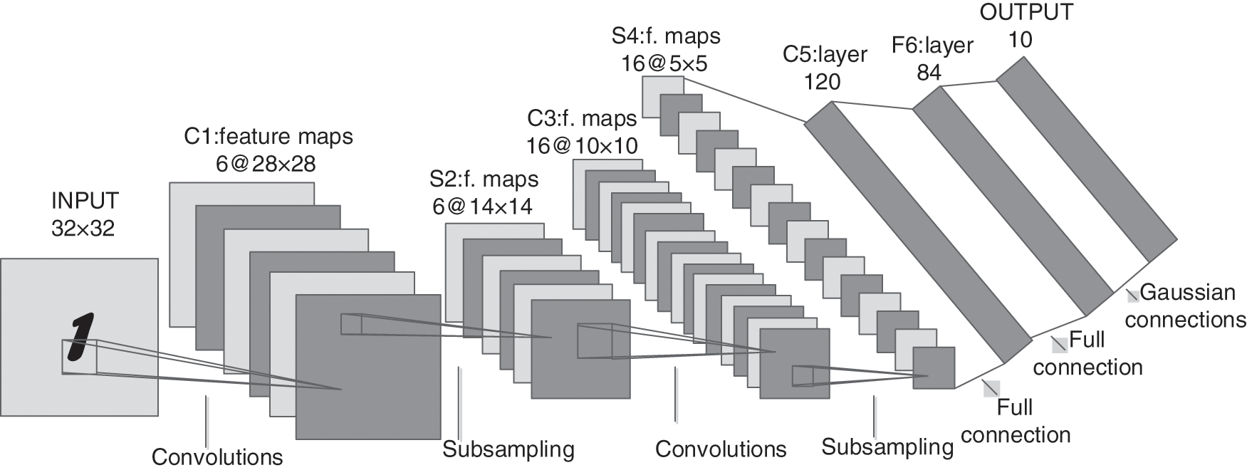
Figure 4: Architecture of LeNet-5
As can be seen from Fig. 4, the network uses 7 layers (excluding input layer). These are 2 convolutional layers, 2 pooling layers, 2 fully connected layers and 1 layer of Gaussian connection. Convolution operations are represented by Convolutions, pooling operations are represented by Subsampling, and full connection operations are represented by Full connection. The original size input is 32 × 32. As a convolutional layer, C1 contains six feature maps, 28 × 28 each. The size of convolution kernel is 5 × 5. S2 is a pooling layer, which reduces the output of the previous convolutional layer from 28 × 28 to 14 × 14. Similarly, C3 is an other convolutional layer. S4 is an other pooling layer. And all the following layers are fully connected layers.
3.2 Design of Convolutional Network for Sugarcane Bud Recognition
Considering the prominent characteristics of sugarcane bud, the proposed model is designed as shown in Fig. 5. The functions of each layer are as follows.
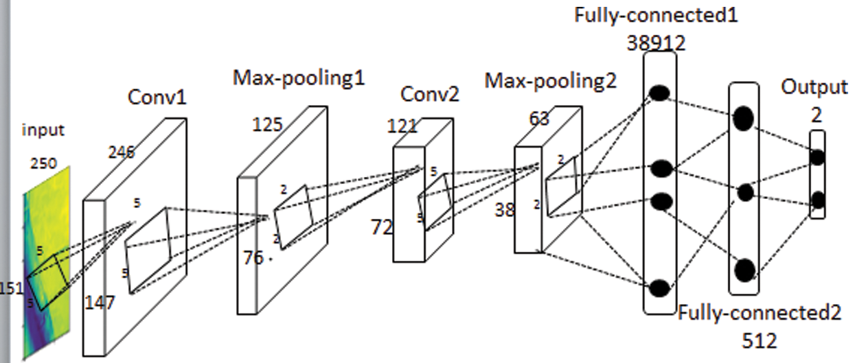
Figure 5: The structure network of sugarcane bud recognition
The first layer is the data input layer. The pixel size of the input image is 250 × 151.
The second layer is Conv1 convolutional layer, which uses 32 filters. The role of convolution kernels is to extract the features of the input image which size is 5 × 5. The total number of parameters to be learned for Conv1 convolutional layer is (5 × 5 + 1) × 32. If the size of the input image is 250 × 151, a feature map with a size of 246 × 147 will be obtained after convolution by a convolution kernel with a stride of 2. Finally, the number of Conv1 convolution layer connections is 832 × (246 × 147). It can be seen that the convolution layer can greatly reduce the number of parameters to be learned by using weight sharing.
The third layer is Max-pooling1 layer (also known as the down-sampling layer). It can be seen from the Fig. 5 that Max-pooling1 layer is connected with convolutional layer Conv1. The feature map size of the Max-pooling1 layer is 1/4 of the output feature map size of the Conv1 convolutional layer.
The fourth layer is Conv2 convolution layer, which uses 64 filters. The role of convolution kernels is to extract the features of the input image. The number of parameters to be learned for Conv2 convolution is (5 × 5 + 1) × 64. And the output feature map size of Conv2 convolution is 119 × 70. So, the total number of connecting lines for Conv2 convolution is 1664 × 119 × 70. All the feature maps of Max-pooling1 layer are convoluted by every convolution kernel of Conv2 convolutional layer, which is the so-called fully connected.
The fifth layer is Max-pooling2 down-sampling layer. Its working principle is the same as that of the previous Max-pooling1 down-sampling layer. The feature mapping output of the Conv2 convolutional layer is processed by the same pooling method.
The sixth layer is Fully-connected1 layer, which has 38912 neurons. Every neuron is connected with all the neurons in the Max-pooling2 sampling layer, which completes the connection of the whole convolutional neural network. The number of feature maps as well as the resolution of feature maps that the network finally outputs to the sampling layer under Max-pooling2 determine the parameters that the Fully-connected1 layer needs to learn.
The seventh layer is Fully-connected2 layer. It is designed into 512 units according to the output. Fully-connected2 layer calculates the dot product of input vector and weight vector, and then adds the offset. It takes the calculated value as the input of the function, and its output is the value of each unit.
The eighth layer is output layer. In fact, this layer is a multi-class SoftMax classifier that determines the number of output nodes according to the classification task. Here, the output is set to 2, so as to achieve the goal of two classification.
3.3 Selection of Activation Function
Linear transformation cannot meet the processing of complex data. And the use of nonlinear transformation can better deal with complex data. The activation function is used in neural network to realize non-linear transformation. Among the three commonly used activation functions, the Sigmoid function [20] and the hyperbolic tangent function Mao et al. [21] are saturated nonlinear function, and the ReLU function [22–24] is unsaturated nonlinear function. Compared with saturated nonlinear function, unsaturated nonlinear function can solve the problem of gradient disappearance and explosion, and can accelerate the convergence speed of model. The activation function used in this paper is the ReLU function. The main reason is that ReLU function is faster and more effective than Sigmoid function and TanH function in solving gradient descent in the designed convolutional neural network. In the case of a large number of training sets, it can greatly reduce the training time of the model. The image of the ReLU function is shown in Fig. 6.
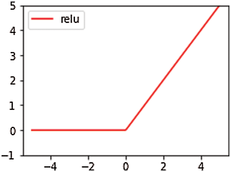
Figure 6: Image of the ReLu function
3.4 Selection of the Loss Function
The cross-entropy function is a very common probability distribution function in the loss function. The model is optimized by calculating the error between the predicted output and the truth. Introducing cross-entropy to measure the training effect of the neural network can solve many problems in the process of neural network classification. In the neural network multi classification problem, the usual method is to set n output nodes and get an n-dimensional array. Each output node in the array corresponds to a label category. The best expectation is that if a sample belongs to category L, the output dimension value of the node corresponding to this category should be 1, and the output of other nodes should be 0. The model in this paper carries out two classifications of sugarcane buds, so its value is a two-dimensional array. If the input image is an image with bad bud, it belongs to category 0. Then the two-dimension value of the network output node is [1,0]. Among them, 1 is the probability of damaged seed bud, which is the result we expect to output.
Cross-entropy is of great significance in defining neural networks as it is used to estimate the length of the average code. The cross entropy is defined by giving two probability distributions p and q as follows:

In the Eq. (1), p(x) and q(x) represent the probability distribution of training samples and predictions respectively. Using cross-entropy as an evaluation metric can make the model output distribution and the training sample distribution as consistent as possible. Many model training results show that the smaller the cross-entropy, the closer the probability distribution of p and q, and the more accurate the expected value of the model. Therefore, the paper uses cross-entropy to measure the error between the output and the truth, and optimizes the model based on this.
After getting the training model, we use the validation set to test its performance, as shown in Fig. 7.
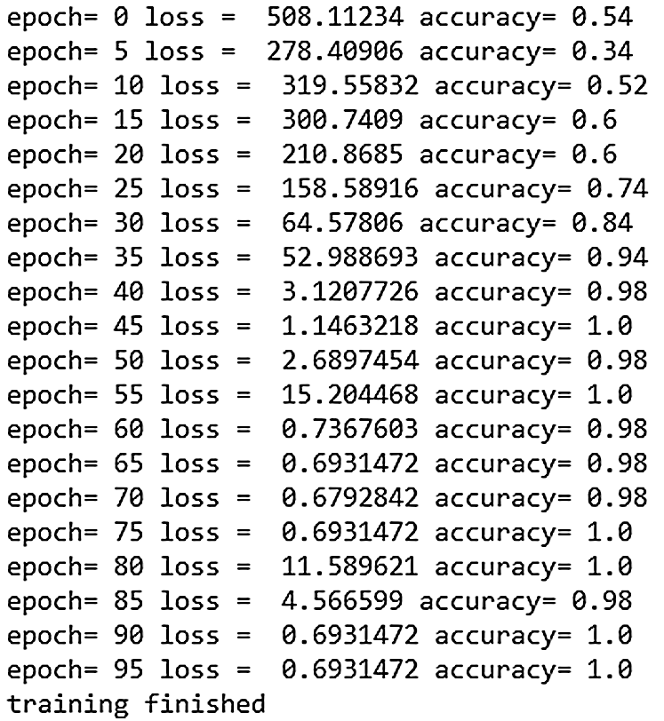
Figure 7: Training loss value and verification accuracy
In Fig. 7, the model accuracy calculated on the validation set each time is obtained by reading the latest saved model. The model is tested every 5 epochs. After the training epoch reaches 90 times, it can be seen that the loss value of the iteration is reduced from 508.11234 to 0.6931472. Although the loss value has fluctuated, it still tends to be smaller overall. It can also be seen from Fig. 7 that the accuracy of the validation set test increased from 0.54 to 0.94 after 35 epochs. The accuracy of the final model is always around 0.99. Since the background of the bud is relatively simple, the training model can quickly learn the features of the training data, and can accurately recognize the conditions of the test image. The experimental results show that the trained model has a good performance. If the choice of learning rate is not good, it is also likely to have a tendency of fitting. There are two ways to prevent the model from overfitting during training. One is to increase the training set, the other is to use the dropout operation. Fig. 8 shows the accuracy of the test set using the dropout operation.
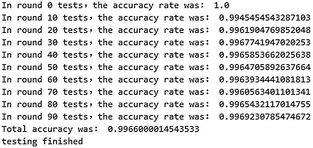
Figure 8: Accuracy list of 100 rounds of tests
If the system model is overfitting, and the number of data sets does not increase, the loss value will no longer decrease regardless of the number of training iterations, and the test accuracy will always be 1.0. It can be seen from Figs. 7 and 8 that the accuracy of the model on the validation set and the test set is not much different, which indicates that the model has a slight overfitting.
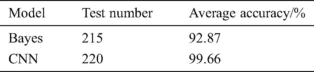
Finally, the model can achieve 95% accuracy through a small number of iterations. The use of the dropout function can prevent the model from overfitting and further improve the accuracy of the model. Fig. 9 shows the training loss curve, and Fig. 10 shows the test accuracy rate curve. The accuracy rate of the test set is also very high, and the sample test rate can generally reach to 0.99, which shows that the performance of the training model is good. We compare the accuracy of sugarcane buds obtained by the CNN model and the Bayesian decision model [8] as shown in Tab. 1. It can be seen that the CNN model has better performance when the test samples are approximately equal.
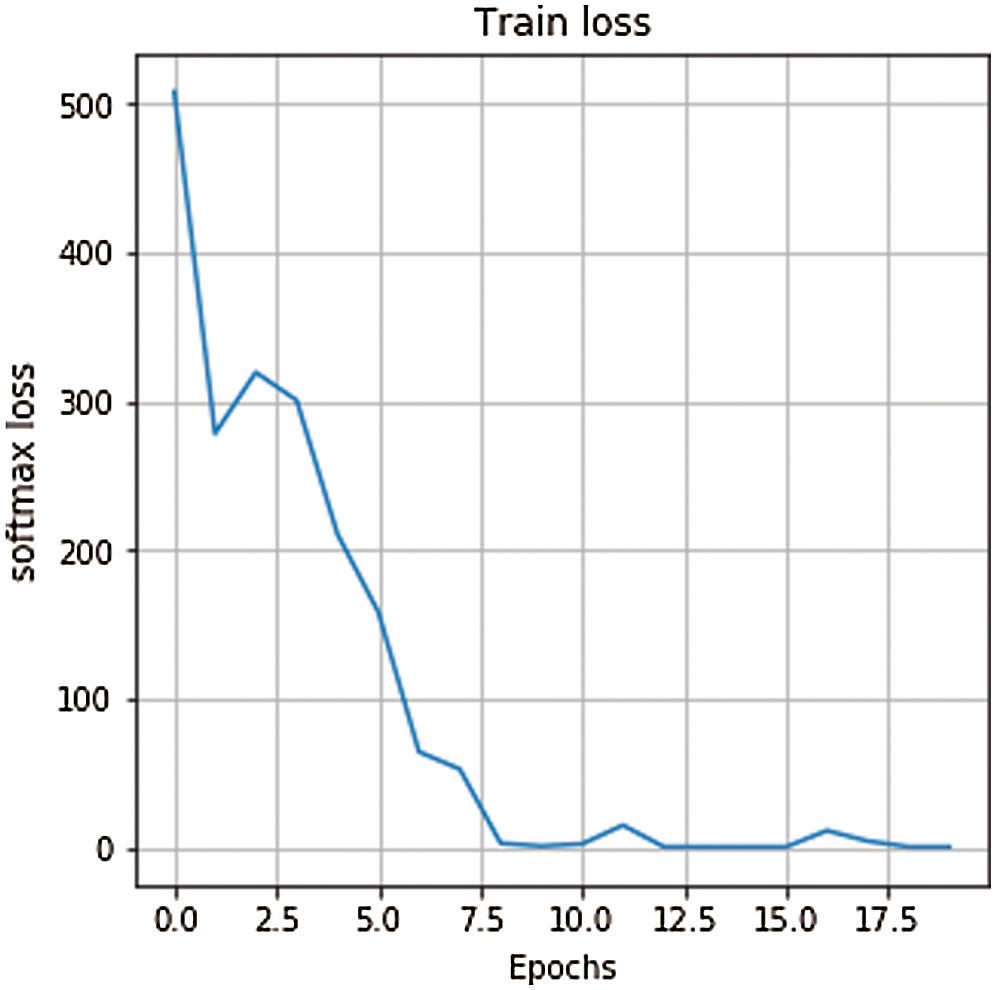
Figure 9: Training loss curve
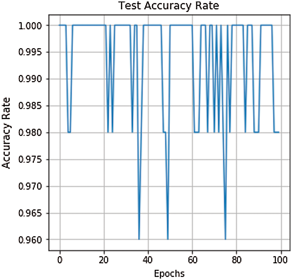
Figure 10: Test accuracy curve
Table 1: Accuracy of bud classification
4.2 Visualization of Convolution Feature
To optimize the model, the convolutional neural networks first propagate the extracted image features forward. Then the difference between the model output and the data label is backpropagated to adjust the network parameters [25]. Since CNN is a black box network, it will increase the difficulty of optimizing network weights. However, if we can display the image features [26] learned by CNN in various layers of networks in the form of images, it will help us to optimize the network parameters more easily. The original input image in the network is shown in Fig. 11.
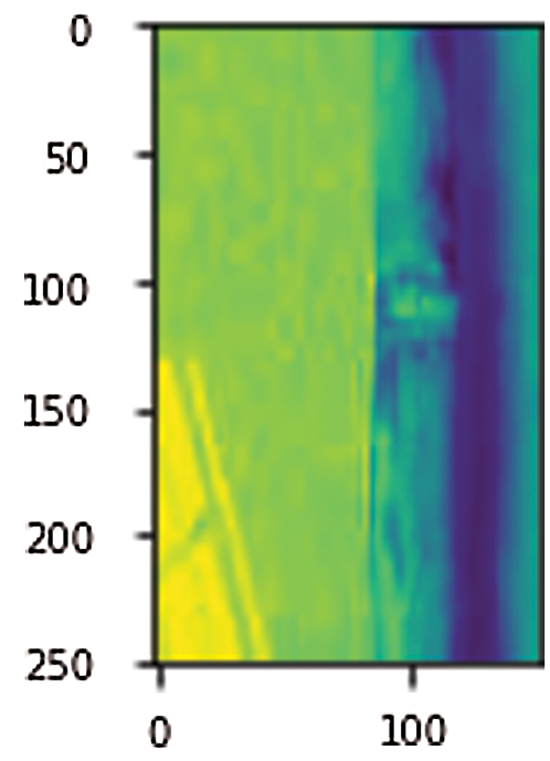
Figure 11: Sugarcane image on input
In the model, 32 filters are used for the first convolution layer Conv1 and the first pooling layer Pool1, 64 filters are used for the second convolution layer Conv2 and the second pooling layer Pool2. Convolution kernels of 5 × 5 are used for Conv1 and Conv2, while convolution kernels of 2 × 2 are used for Pool1 and Pool2. We select 9 feature maps from each layer, and the visualization results are shown in Fig. 12.
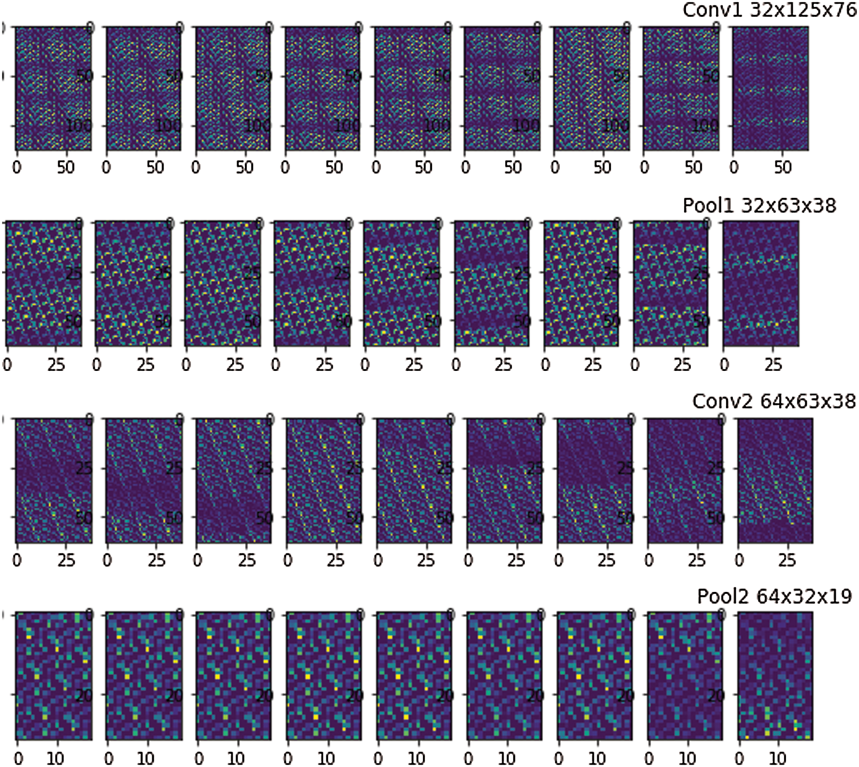
Figure 12: Visualization results of convolution and pooling
It can be seen from Fig. 12 that the filter of the convolutional layer Conv1 mainly extracts the underlying feature information of the color, texture and direction of the image. The filter of the pooling layer Pool1 further extracts the image texture and direction on the basis of Conv1. Pool1 can reduce the parameter value of the model by reducing the size of the feature map. Similarly, Conv2 continues to extract deeper texture and direction information from the feature map output by Pool1. This is more conducive to the model to learn the main features of the image. The visual patterns of lines, directions, and textures observed in Fig. 12 are very regular, which indicates that the features extracted by the model are very obvious.
In this paper, the CNN model is constructed to recognize the conditions of sugarcane buds. Compared with the traditional sugarcane bud recognition technology, this method greatly reduces the work of artificially extracting seed bud characteristics during image recognition. The model designed in this paper has better recognition accuracy than the traditional image processing method. There are two reasons for the high recognition rate. One is that the sugarcane bud images are collected under a single background, so the characteristics of the bud are not disturbed by complex background features. It can be seen from Fig. 12 that the extracted image features are very regular. The second is that deep learning has excellent performance in image recognition. The experiments results show that the recognition accuracy of the model reaches to 99%. A higher recognition rate will effectively reduce the production cost and improve the economic benefits of sugarcane.
Funding Statement: The authors are highly thankful to the Research Project for Young and Middle-aged Teachers in Guangxi Universities (ID: 2019KY0621), to the Natural Science Foundation of Guangxi Province (No. 2018GXNSFAA281164). This research was financially supported by the project of outstanding thousand young teachers’ training in higher education institutions of Guangxi, Guangxi Colleges and Universities Key Laboratory Breeding Base of System Control and Information Processing. Thanks for Key scientific research project of Hechi University (No. 2018XJZD004).
Conflicts of Interest: The authors declare that they have no conflicts of interest to report regarding the present study.
1. J. Wang and J. Y. Guo. (2013). “Sugarcane cultivation management technology,” Agricultural Technology Services, vol. 30, no. 24, pp. 321–322. [Google Scholar]
2. Z. Y. Zhang. (2018). “Analysis and application of sugarcane planting technology,” Agriculture and Technology, vol. 38, no. 16, pp. 64–69. [Google Scholar]
3. K. Moshashai, M. Almasi, S. Minaei and A. M. Borghei. (2008). “Identification sugarcane nodes using image processing and machine vision technology,” International Journal of Agricultural Research, vol. 3, no. 5, pp. 357–364. [Google Scholar]
4. S. P. Lu. (2011). “Recognition of sugarcane stem nodes and detection of sugarcane buds based on machine vision,” Ph.D. dissertation. Huazhong Agricultural University, China. [Google Scholar]
5. S. P. Lu, M. C. He, X. Huang and C. L. Cui. (2012). “Recognition of sugarcane nodes based on image gray statistical gradient characteristics,” Guangxi Agricultural Mechanization, 6, pp. 21–22. [Google Scholar]
6. W. Z. Zhang, S. Y. Dong, X. X. Qi, Z. J. Qiu, X. Wu et al. (2016). , “The identification and location of sugarcane internode based on image processing,” Agricultural Research, 4, pp. 217–221. [Google Scholar]
7. Y. Q. Huang, X. B. Wang, K. Yin and M. Z. Huang. (2015). “Design and experiments of buds-injury-prevention system based on induction-counting in sugarcane-seeds cutting,” Transactions of the Chinese Society of Agricultural Engineering, vol. 31, no. 18, pp. 41–47. [Google Scholar]
8. Y. Q. Huang, K. Yin, M. Z. Huang, X. B. Wang and Z. Y. Luo. (2016). “Detection and experiment of sugarcane buds integrity based on Bayes decision,” Transactions of the Chinese Society of Agricultural Engineering, vol. 32, no. 5, pp. 57–62. [Google Scholar]
9. A. Krizhevsky, I. Sutskever and G. E. Hinton. (2012). “ImageNet classification with deep convolutional neural networks,” in Proc. Advances in Neural Information Processing Systems, Lake Tahoe, USA, pp. 1090–1098. [Google Scholar]
10. C. Farabet, C. Couprie, L. Najman and Y. Lecun. (2013). “Learning hierarchical features for scene labeling,” IEEE Transactions on Pattern Analysis and Machine Intelligence, vol. 35, no. 8, pp. 1915–1929. [Google Scholar]
11. J. Tompson, A. Jain, Y. Lecun and C. Bregler. (2014). “Joint training of a convolutional network and a graphical model for human pose estimation,” in Proc. Advances in Neural Information Processing Systems, Montreal, Canada, pp. 1799–1807. [Google Scholar]
12. T. Dobhal, V. Shitole, G. Thomas and G. Navada. (2015). “Human activity recognition using binary motion image and deep learning,” Procedia Computer Science, vol. 58, pp. 178–185. [Google Scholar]
13. C. A. Ronao and S. B. Cho. (2016). “Human activity recognition with smartphone sensors using deep learning neural networks,” Expert Systems with Applications, vol. 59, pp. 235–244. [Google Scholar]
14. S. Zhang, W. Huang and C. Zhang. (2019). “Three-channel convolutional neural networks for vegetable leaf disease recognition,” Cognitive Systems Research, vol. 53, pp. 31–41. [Google Scholar]
15. L. S. Fu, Y. L. Feng, T. Elkamil, Z. H. Liu, R. Li et al. (2018). , “Image recognition method of multi-cluster kiwifruit in field based on convolutional neural networks,” Transactions of the Chinese Society of Agricultural Engineering, vol. 34, no. 2, pp. 205–211. [Google Scholar]
16. Z. H. Zhao, H. Song, J. B. Zhu, L. Lei and L. Sun. (2018). “Identification algorithm and application of peanut kernel integrity based on convolution neural network,” Transactions of the Chinese Society of Agricultural Engineering, vol. 34, no. 21, pp. 195–201. [Google Scholar]
17. L. Zhu, Z. B. Li, C. Li, J. Wu and J. Yue. (2018). “High performance vegetable classification from images based on alexnet deep learning model,” International Journal of Agricultural and Biological Engineering, vol. 11, no. 4, pp. 217–223. [Google Scholar]
18. R. S. Zhu, X. H. Yan and Q. S. Chen. (2020). “Study on the optimization of soybean seed selection based on image recognition and convolution neural network,” Soybean Science, vol. 39, no. 2, pp. 189–197. [Google Scholar]
19. Y. Lecun, L. Bottou, Y. Bengio and P. Haffner. (1998). “Gradient-based learning applied to document recognition,” Proceedings of the IEEE, vol. 86, no. 11, pp. 2278–2324. [Google Scholar]
20. Y. N. Zhang, J. W. Chen, J. R. Liu, L. Qu and W. B. Li. (2013). “Unipolar sigmoid neural network classifier based on weights and structure determination,” Journal of Computer Applications, vol. 33, no. 3, pp. 766–770. [Google Scholar]
21. H. J. Mao, W. Li and X. L. Feng. (2016). “Design of nonlinear tracking differentiator based on hyperbolic tangent,” Computer Application, vol. 36, no. S1, pp. 305–309. [Google Scholar]
22. Y. H. Mao, X. L. Gui, Q. Li and X. S. He. (2016). “Deep learning application technology research,” Computer Application Research, vol. 33, no. 11, pp. 3201–3205. [Google Scholar]
23. Y. Lecun, B. E. Boser, J. Denker and D. Henderson. (1990). “Handwritten digit recognition with a back-propagation network,” in Proc. Advances in Neural Information Processing Systems, Denver, USA, pp. 267–285. [Google Scholar]
24. V. Nair and G. E. Hinton. (2010). “Rectified linear units improve restricted Boltzmann machines,” in Proc. Int. Conf. on Machine Learning, Haifa, Israel, pp. 807–814. [Google Scholar]
25. Z. W. Wu. (2015). “Application of convolutional neural network in image classification,” Ph.D. dissertation. University of Electronic Science and technology, China. [Google Scholar]
26. Y. L. Boureau, J. Ponce and Y. Lecun. (2010). “A theoretical analysis of feature pooling in visual recognition,” in Proc. Int. Conf. on Machine Learning, Haifa, Israel, pp. 111–118. [Google Scholar]
 | This work is licensed under a Creative Commons Attribution 4.0 International License, which permits unrestricted use, distribution, and reproduction in any medium, provided the original work is properly cited. |