DOI:10.32604/iasc.2021.015932
| Intelligent Automation & Soft Computing DOI:10.32604/iasc.2021.015932 | |
| Article |
Multi-Model Fuzzy Formation Control of UAV Quadrotors
1Systems Engineering Department, King Fahd University of Petroleum & Minerals, Dhahran, 31261, Saudi Arabia
2Centre de Développement des Technologies Avancées, Algeria
*Corresponding Author: Mujahed Al-Dhaifallah. Email: mujahed@kfupm.edu.sa
Received: 14 December 2020; Accepted: 14 January 2021
Abstract: In this paper, the formation control problem of a group of unmanned air vehicle (UAV) quadrotors is solved using the Takagi–Sugeno (T–S) multi-model approach to linearize the nonlinear model of UAVs. The nonlinear model sof the quadrotor is linearized first around a set of operating points using Taylor series to get a set of local models. Our approach’s novelty is in considering the difference between the nonlinear model and the linearized ones as disturbance. Then, these linear models are interpolated using the fuzzy T–S approach to approximate the entire nonlinear model. Comparison of the nonlinear and the T–S model shows a good approximation of the system. Then, a state-feedback controller is synthesized utilizing the parallel distributed compensation (PDC) concept. The linear quadratic regulator (LQR) controller is used to stabilize the system and obtain the desired response. This is followed by the formation control of a set of quadrotors using the leader–follower method. In this strategy, the potential field method is utilized to obtain the ideal shape formations. An attractive potential is generated such that the followers are attracted towards the leader, and a repulsive potential is generated that repels adjacent quadrotors to avoid collisions. Simulations are performed to evaluate the proposed method’s effectiveness in obtaining the desired shape formation for different cases. From the simulation results, we can see that the proposed formation control results in a good tracking response.
Keywords: Multi-models; nonlinear systems UA quadrotor; fuzzy logic control; formation control
Unmanned air vehicles (UAVs) have attained significant attention and progress in the past decade due to their innumerous advantages and applications. A UAV is an airborne robot that can fly autonomously or semi-autonomously without a pilot on board. The tasks that are needed to be performed by the UAVs are given through a control system that may be mounted on the vehicle or somewhere else. UAVs consist of multivariable nonlinear dynamics whose complexity depends on the required operation and objectives.
Due to their reliability, UAVs can replace manned aerial vehicles in many areas, such as civilian communities, agriculture, and military. In the military, UAVs are utilized to convey various loads, such as radars, sensors, cameras, or weapons. In addition, UAVs can be utilized for observation and exploring unfriendly environments [1]. Outside of the military, UAVs are valuable for several applications, such as watching regular assets, home security, scientific research, and search and rescue operations.
The concept of “Divide and Conquer” is generally used to solve complex problems in day-to-day life. The problem can be divided into several more manageable parts, which, when solved individually and combined, can give the solution to the entire problem. A similar concept can even be used in controlling nonlinear systems. The complex nonlinear model can be divided into a set of locally linearized models and then interpolated to obtain the overall system. This method is called the multi-model approach (MMA), also known as Takagi–Sugeno (T-S) modeling [2]. The interpolation of all the individual models is done using fuzzy logic.
Recently, the utilization and control of groups of UAVs to accomplish certain tasks cooperatively has attracted much interest from researchers in related fields. This is a direct result of the advantages acquired from utilizing numerous vehicles as opposed to utilizing a more elaborated single vehicle. Comparing the outcome of performing a task with a team of UAVs with that of a single vehicle, one can realize that the overall performance of multiple UAVs is more efficient and safer.
The formation of a multi-UAV is a combination of the study of both quadrotors and synchronization. It has received considerable interest from both autonomous systems and control groups. Cooperative coordination can be described as a set of UAVs assigned to follow a predefined path of flight while obtaining useful information through their sensors and maintaining a prescribed formation structure. The trajectory of the flight could be a set of coordinates that the UAVs must follow or a prescribed region of fly within certain boundaries (see, e.g., [3,4] and the references therein).
There has been much research and contribution to quadrotor UAVs. One of the earliest works is by Samir Bouabdallah in [1,5], where he formulated the dynamics of the quadrotor model and presented briefly different control techniques applied to it. The dynamics modeling, simulation, and system identification has also been addressed in other papers like [6,7]. The application of a simple proportional-integral-derivative (PID) controller for the quadrotor is given in Jithu et al. [8]. Attitude control techniques using observers are given in Xu et al. [9].
Many nonlinear techniques have been employed on the quadrotors to stabilize the system. In Mistler et al. [10], a feedback linearization method was developed to control the quadrotor and track a predefined trajectory. Voos [11] developed a control structure based on feedback linearization and its decomposition into a nested structure. A backstepping method was proposed by Altug et al. [12] in which the positions and the yaw angle were kept constant while the pitch and the roll angle regulate to zero to stabilize the quadrotor. Zuo [13] employed the backstepping technique with command-filtered compensation. Sliding mode techniques were developed in Xu et al. [14], and a combination of sliding mode control and backstepping technique has been considered in Bouadi et al. [15]. Stabilization of the attitude of the UAV based on the compensation of the Coriolis and gyroscopic torques has been studied in Tayebi et al. [16].
Applications of fuzzy theory in control systems are widely seen in the literature. The T–S model, which uses the MMA for the quadrotor, is shown in Takagi et al. [2]. The concept of approximation based on multiple models is not new. Since Johansen and Foss’s work and publications on this topic, the MMA has obtained significant attention [5]. Initially, certain authors tried to represent nonlinear systems using piecewise linear approximations [17], which use local models and switching. A few years later, Takagi et al. [2] presented the multi-experts approach that combines different experts via activation functions (where an expert is a model describing the local behavior of a system).
Cooperative control of multiple UAVs, known as formation control, is an important issue in real applications and research. When the formation changes its shape from the mission requirements, it is necessary to control the relative position, attitude, and speed between UAVs to avoid a collision. The most common formation method used is the leader–follower technique.
In the leader–follower method, an individual is selected to be the leader, and the others are followers [18]. Rarely, in some situations, multiple agents are considered leaders [19]. The followers must locate themselves and maintain a desired position relative to the leader [20]. Control frameworks with the leader–follower methodology show satisfactory performance. Simplicity and reliability are the characteristics of this technique. Nonetheless, the disadvantage of this technique is that the leader does not receive feedback from the followers.
Leader–follower formation control strategies have been examined generally, including different procedures like PID control approach [21] and decentralized control based on the linear quadratic regulator (LQR) [22]. The leader–follower approach was investigated in Guerrero et al. [23], where a nonlinear controller was designed by combining nested saturations with consensus control to achieve the formation of mini rotorcrafts. Turpin et al. [24] reported a formation where the vehicles track a given trajectory. The quadrotors can change the formation shape safely as per determinations. Shape vectors prescribe the formation and keep the relative separations and direction between the quadrotors. In Ru et al. [25], a multi-model predictive control technique was used on the leader–follower formation of the quadrotor flying in two dimensions by using fuzzy logic. A simplified nonlinear model is used in this study.
In this paper, a complete dynamic model was used, and a new technique was used to obtain the linear models. The difference between the linear model obtained from the Taylor series linearization method and the actual nonlinear system at an operating point was added to the linear system and considered a disturbance when designing the controller. Satisfactory results were obtained.
The paper is organized as follows. Section 2 presents the mathematical model of the UAV. Section 3 is devoted to the linearization and the T–S modeling of the quadrotor. The formulation of the fuzzy controller with the LQR technique is summarized in Section 4. The leader–follower formation is described in Section 5. Section 6 presents the simulation results obtained in this study. Section 7 concludes the paper.
2 Quadrotor Dynamics and Mathematical Modelling
The quadrotor consists of four rotating propellers driven by four DC motors that govern the vehicle’s motion. The quadrotor’s orientation is determined by the Euler angles, which are the roll angle (φ), pitch angle (θ), and yaw angle (ψ). The dynamics of the quadrotor can be explained in Fig. 1. The system consists of the inertial frame Rb and the body frame Rm as shown. The forces appearing on the quadrotor are the roll, pitch, and yaw torques and the total thrust force.
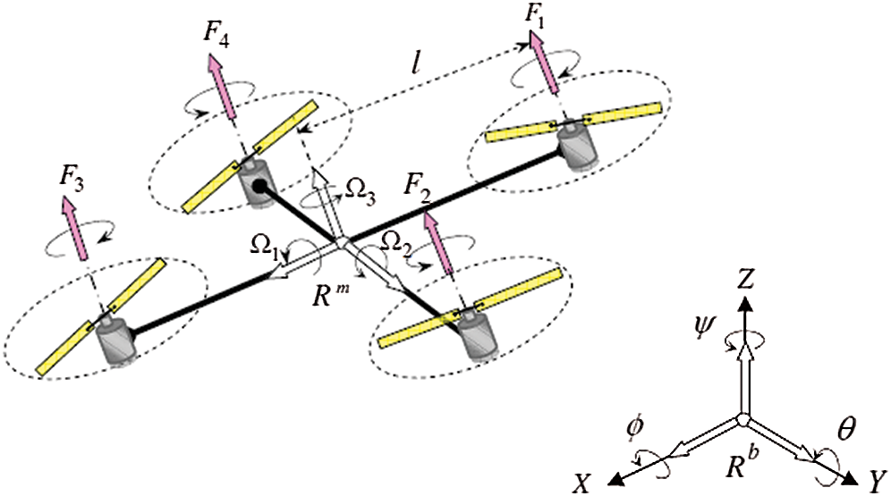
Figure 1: Quadrotor dynamics
The transformation matrix used for the transformation of the system from the inertial or ground frame to the body frame in terms of the Euler angles is:

where s(x) and c(x) represent sin(x) and cos(x), respectively.
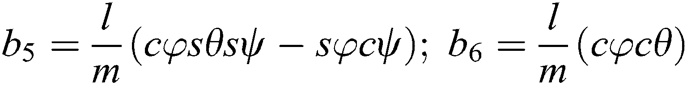
Now, by considering the Euler angles of rotation and Newton–Euler or Lagrange method of developing models, the equations of motion are derived in terms of the translational and rotational parameters, which are [φ, Ө, ψ, x, y, z]. Thus, the set of nonlinear equations obtained are:
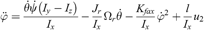
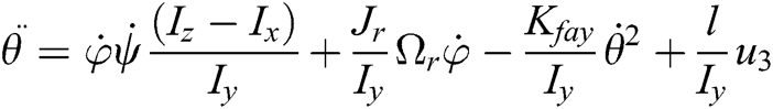

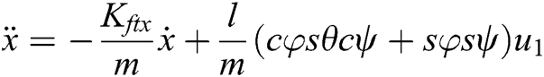
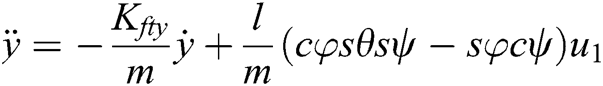
where l is the length of each arm, and m is the mass of the quadrotor. Ix, Iy, and Iz are the moments of inertia around x, y, and z axes, respectively. u1, u2, u3, and u4 are the control inputs.
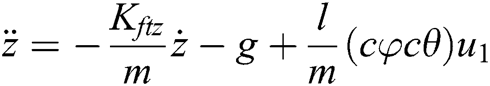
The control inputs are related to the angular velocities of the rotors by the following relation:

where b is the thrust, and d is the drag parameter. ωi is the angular velocity of the ith rotor.
3 Quadrotor Takagi-Sugeno Modelling
In this section, the T–S models for the UAV will be generated by first linearizing the nonlinear model given in Eq. (2). Details of the linearization are provided in subsection 3.1. The T–S model for the UAV is formulated in Subsection 3.2. Subsection 4.3 present the validation of the T–S model.
The linearized model is obtained using the T–S representation, which involves the MMA. It is based on the “Divide and Conquer” rule. According to the MMA, the complete nonlinear complex system is divided into several simpler linear sub-systems. The solutions of these sub-systems, when combined, should give the solution of the complete system. Generally, the complex system is divided into linear models that describe the system’s dynamics in different regions of the operating space. The entire system can be achieved by interpolation.
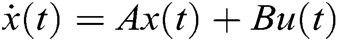
For convenience, the nonlinear model of the quadrotor is represented in state-space form as follows:


The state, input, and output vectors are:


To obtain the state matrices A, B, C, and D, the Taylor series linearization process is used.
The behavior of the nonlinear system about an operating point (xi,ui) can be approximated by a linear time-invariant system (LTI system). We use the Taylor series of the first order to obtain:

which can be written as:

where:


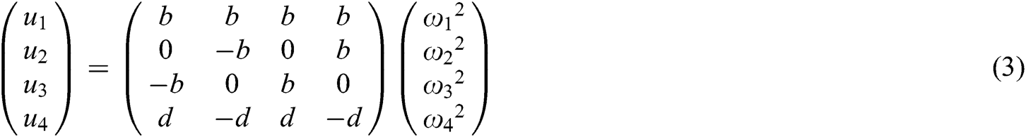
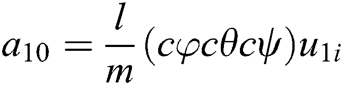
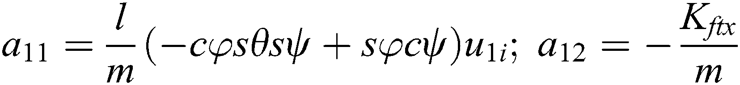
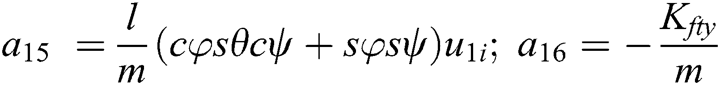
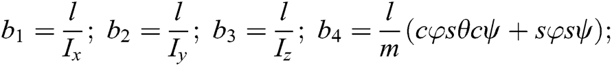
Therefore, by performing the above derivation, the matrices Ai and Bi are obtained as:
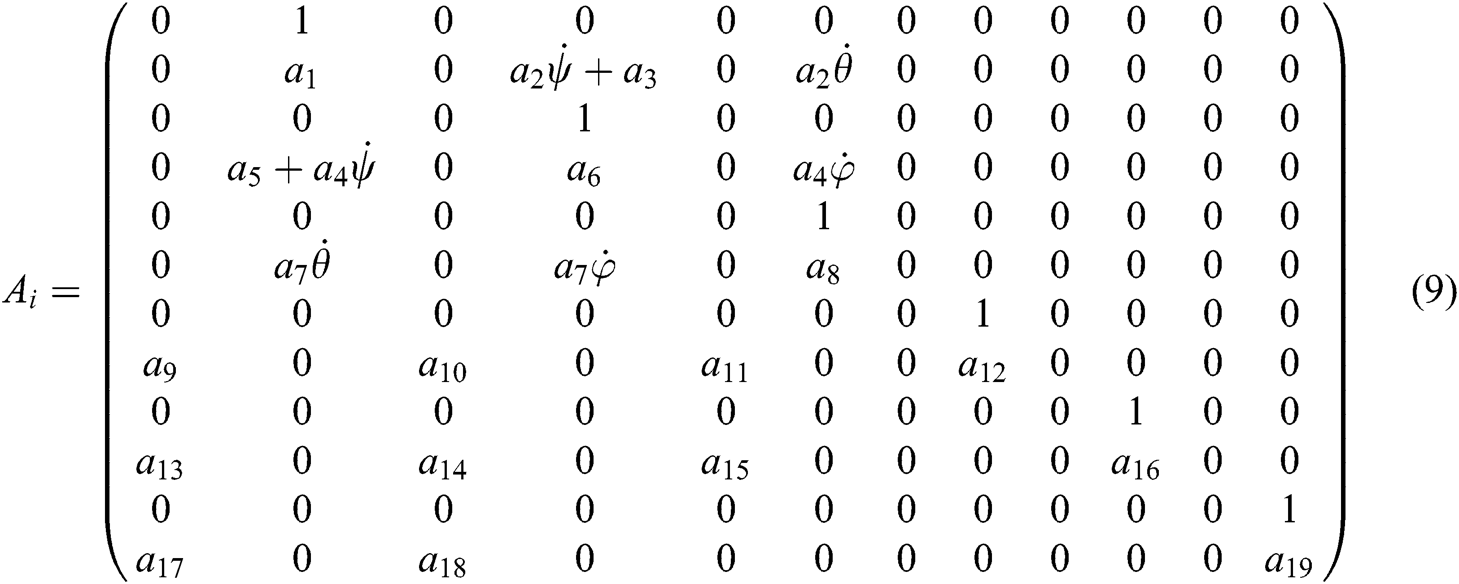
where,
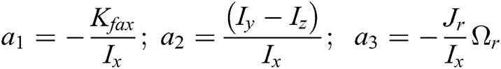
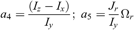
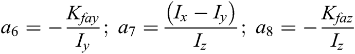
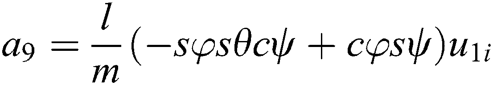


where,
The matrix C(x) is taken as an identity matrix, and D is taken as zero.
3.2 Takagi–Sugeno Model Design
To build the T–S model, we use  locally linearized models. These models are interpolated using the T–S fuzzy logic. The architecture and formulation of the model are described in Fig. 2 below.
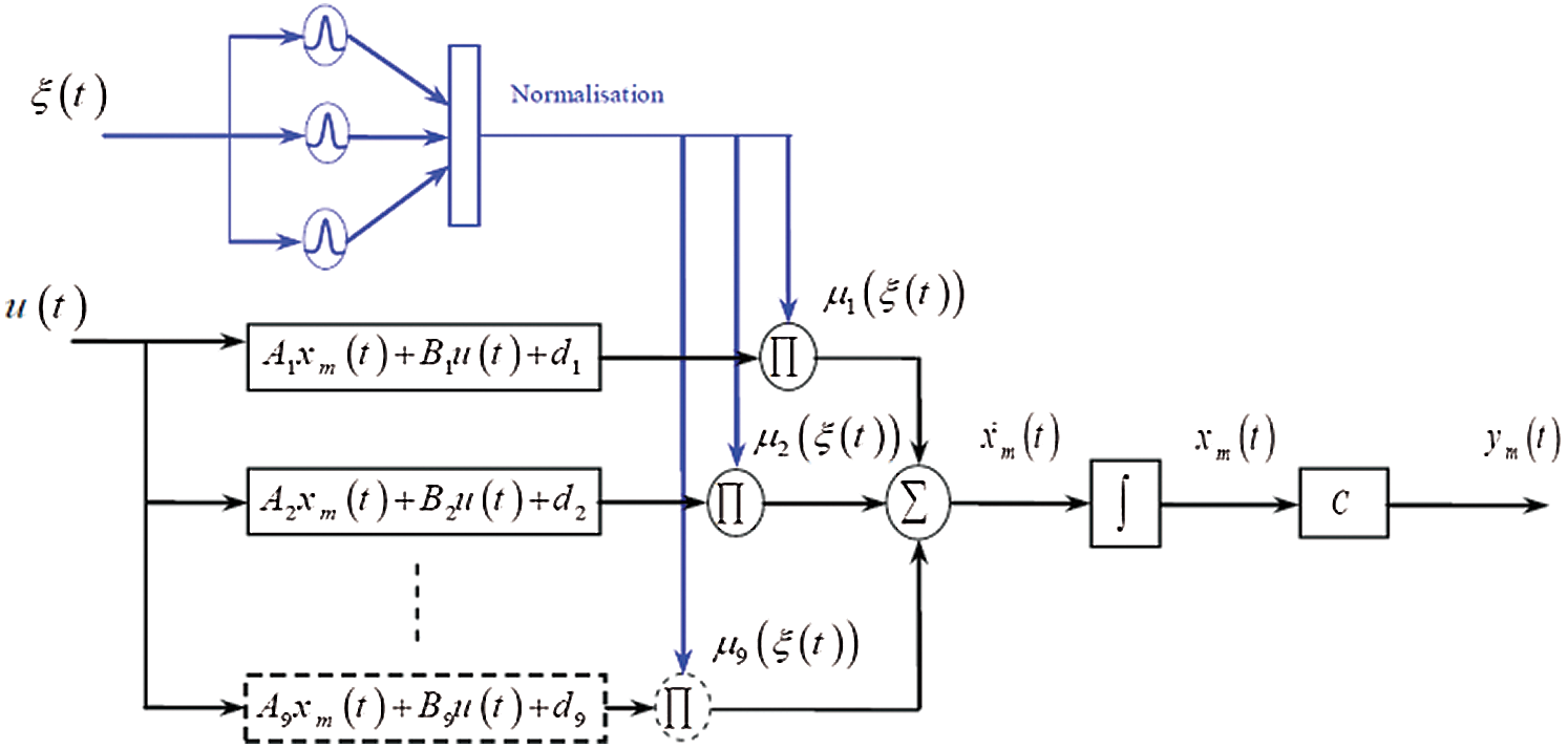
Figure 2: Takagi–Sugeno architecture for multi-models
The linearized models are given as:
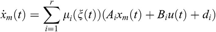

where r is the number of local linear models, x, y, and u are the state, output, and input vectors, respectively. A and B are the state and input matrices, ξ(t) is the fuzzy decision variable, and 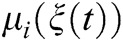 is the normalized activation function.
The activation function determines the degree of activation of the individual local model. It shows the amount of contribution of each local model to the entire system. The properties of the activation function are as follows:
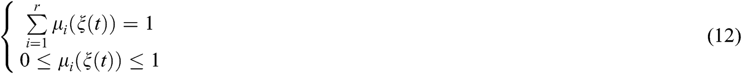
Different types of activation functions can be used in fuzzy theory, such as Triangular, Sigmoidal, and Gaussian. In this work, we use the Gaussian activation function, which is defined as follows:

where m is the dimension of the decision variables vector ξ(t). Mij is the membership functions defined based on the Gaussian fuzzy rules as follows:

where  represents the member function center, and
  determines the member function width. The individual models are defined around the operating points as follows:
• Three models are defined around the roll angle, φ = −300, 00, 300
• Three models are defined around the pitch angle, θ = −300, 00, 300
• Three models are defined around the yaw angle, ψ = −600, 00, 600
The decision variable vector is taken as,

3.3 Validation of the Takagi-Sugeno Model
To validate the T–S model, we use a pseudo-random binary signal (PRBS) as input to both the nonlinear model given in Eq. (2) and the T–S model given in Eq. (11). Then, we simulate the two systems in parallel, and the results are compared.
The amplitude of the PRBS can be very low, but it must be above the residual noise. If the signal to noise ratio is too low, it is necessary to increase the simulation’s duration to get a good estimate of the parameters. A typical value of the amplitude of the PRBS is 0.5%–5% of the value of the operating point on which it is applied, namely:

where
The PRBS can be generated in MATLAB Simulink using the predefined function block. The signals are generated as shown in Fig. 3.
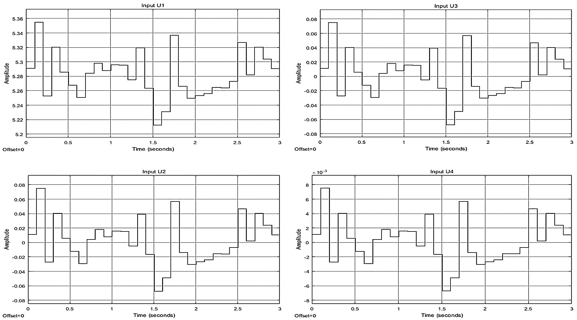
Figure 3: PRBS input signals
The parameters of the quadrotor used in the simulations are taken from [2] and given in Tab. 1 as follows:
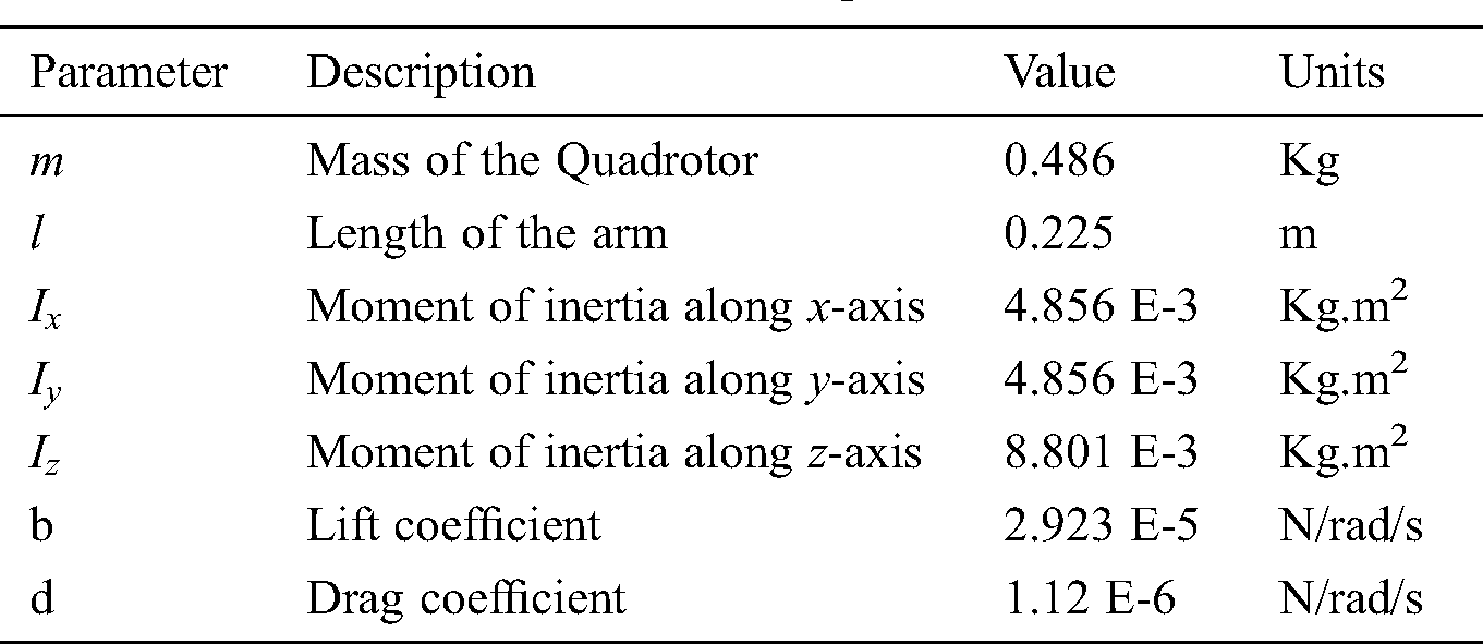
The simulation of the nonlinear and the T–S models with PRBS inputs are carried out in MATLAB using all the parameters described. The behavior of all the states with the given inputs is obtained as shown in Fig. 4.
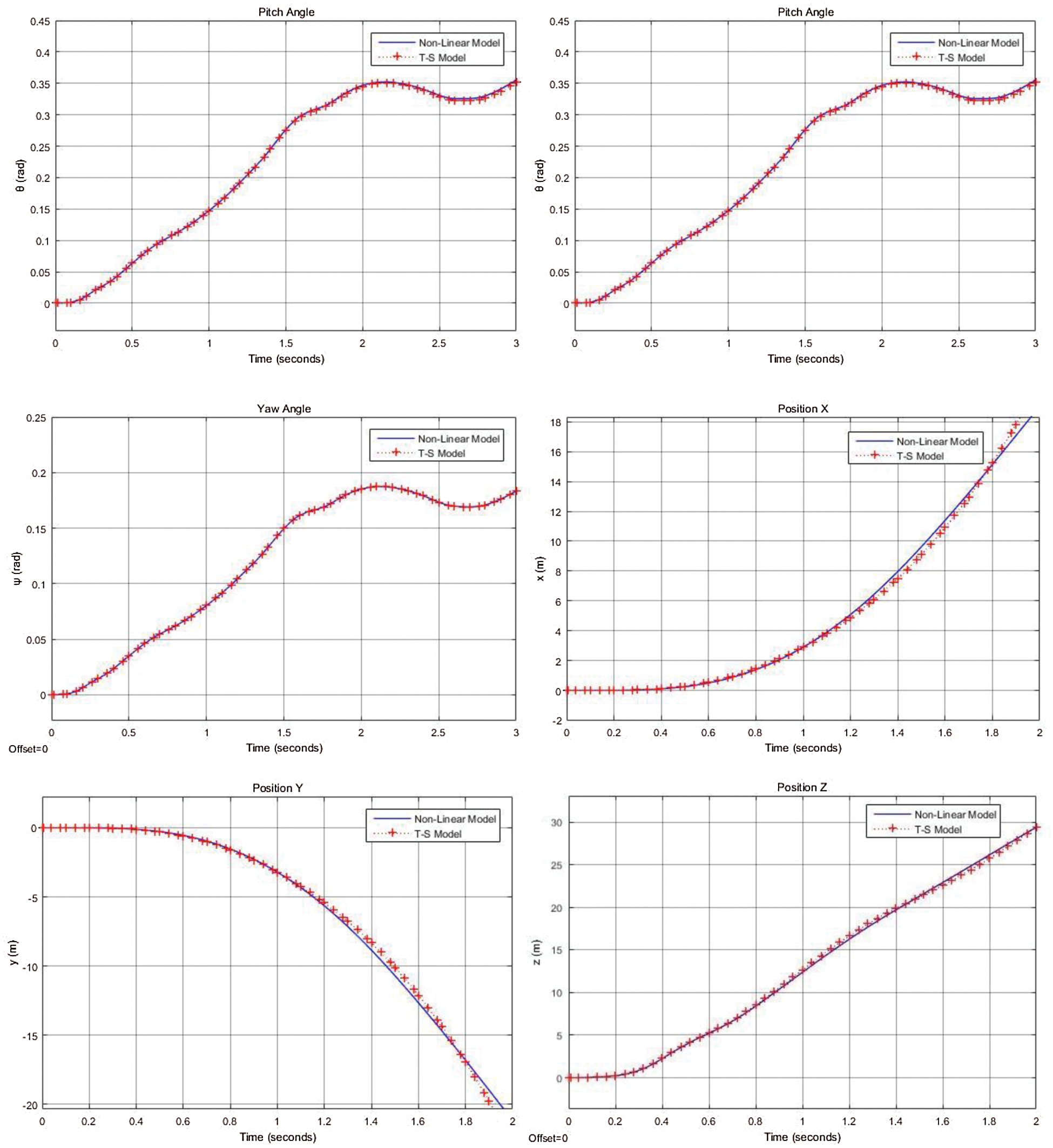
Figure 4: States of the quadrotor nonlinear model vs. T–S model
Therefore, it can be observed that the T–S model gives a good approximation of the dynamics of the nonlinear quadrotor model within a range of operating points assumed.
In this work, because we use the T–S system, the parallel distributed compensation (PDC) technique is used to develop the control law for multi-models. In PDC, the control design utilizes the multiple-model approach to mirror the structure of the T–S model. Consider the T–S model that has been discussed earlier:


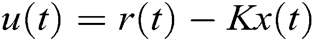
Now, we define the control law u(t) as follows:

where r(t) is the desired states function, and Ki is the state-feedback gain of the ith model. Thus, the closed-loop system becomes:

Notably, the controller parameters, such as Ai, Bi, and activation functions, are respectively the same as the parameters of T–S models.
The quadrotor is a MIMO system that cannot be controlled easily by simple pole placement techniques. Therefore, optimization techniques are essential to stabilize the system and reach the desired states. The solutions of optimal control provide an automated design technique in which only the figure of merit is required [9]. The most widely used method is LQR optimization because of its good efficiency. In this work, we use the LQR technique to obtain the state-feedback gains of the controller described in Eq. (18).
Consider a general plant with the state-space equations and control law as follows:

Now, to obtain the gain K, we define a cost function such that it is the sum of the penalties of the states and the input. These penalties represent how far the system is from the desired response. This can be represented as:

This cost function J is now minimized to reduce the penalties of the controller. This implies Q and R, are both selected as positive definite matrices. The gain K is calculated as:

where P is obtained by solving the algebraic Riccati equation:

Now, the same procedure can be applied to our T–S state feedback controller. All the gains can be calculated as:
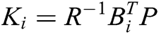

where  , and
, and  is the number of T–S models.
5.1 Leader–Follower Formation Scheme
Consider a system consisting of one leader quadrotor and N follower quadrotors. It is assumed that all these quadrotors have identical models and controllers, as discussed before. The T–S model for each quadrotor can be represented as:
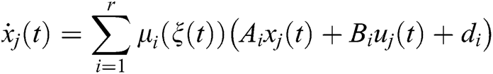

j =0,1, 2,…,N are the number of quadrotors.
Now, the state feedback LQR controllers for the quadrotors are given as:

where  is the reference trajectory for each quadrotor, and Ki is the state feedback gains calculated using LQR.
To obtain the leader-follower formation, the reference signal for the leader r0(t) is selected as per our desired required response. However, the reference signals for the followers, rj(t), j = 1,2,…,N are defined as the trajectory of the leader with some offsets. This can be represented as:

where  is the current state vector of the leader, and
  is the offset for all the states of the jth follower with respect to the leader. Therefore, the control law for each follower becomes:

Therefore, the closed-loop system for each follower becomes:

It should be noted that all the parameters of the fuzzy functions and the states are identical for all the quadrotors. Additionally, in practice, the control of only the positions (x, y, z) is performed, and the rest of the states of the quadrotors are set to track the leader. This means that the offsets are present only for the position states of the reference signals.
5.2 Potential Fields Technique for Shape Formation
Potential fields technique is used to obtain cooperative control of the quadrotors. Each follower has information on the positions of the leader and adjacent followers. Using this information, an attractive and a repulsive potential force is applied on each follower to obtain the desired shape formation. The followers are attracted towards the leader via the attractive potential. The repulsive potential repels adjacent followers and keeps them at a specified distance d. Therefore, two potential field functions are defined based on this concept: one is Uatt, the attractive potential, and the other is Urep, the repulsive potential. These functions are defined as follows:

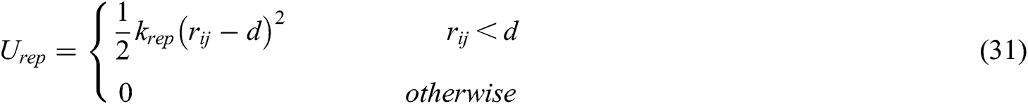
where  is the current distance between the leader, and the ith follower,
  is the current distance between the ith and the jth followers, R is the required distance between the leader and the followers, d is the desired distance between each adjacent follower, and
  are positive tuning constants.
Now, the forces associated with each potential are calculated as a negative gradient of the above functions. The overall force applied on each follower is represented as:

where

and

The control scheme described above can be illustrated as shown in Fig. 5.
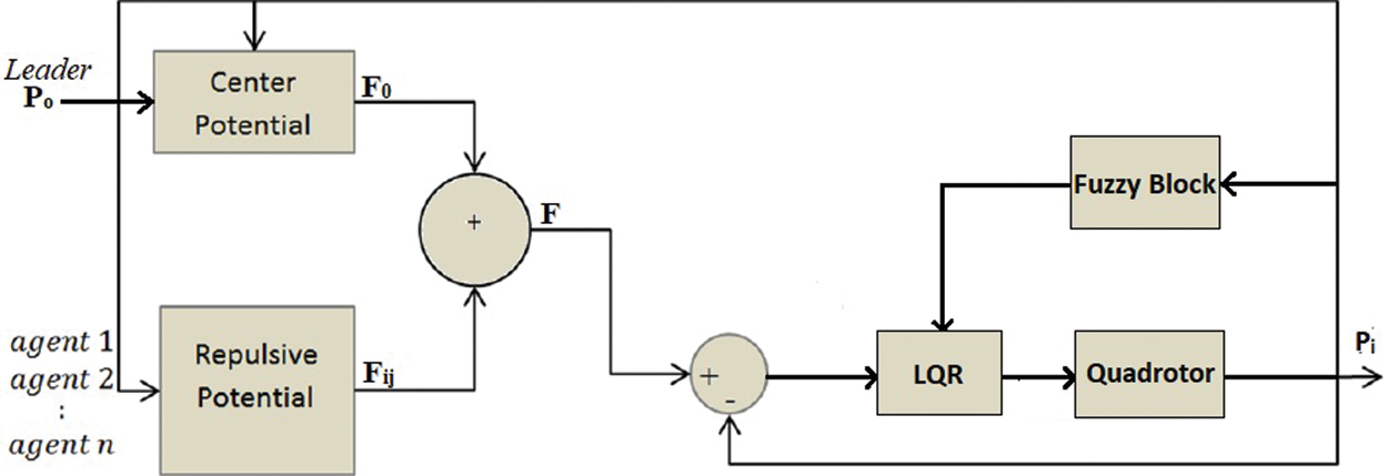
Figure 5: Control scheme of a follower quadrotor using potential fields
The center and the repulsive potentials are obtained by applying the gradient, as discussed above. After computation, they are obtained as follows:


where P’s are the position vector of the quadrotors defined as:
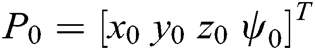 for the leader,
  , and
, and 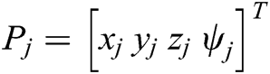 for adjacent followers i,j.
The entire control scheme explained in the previous sections is implemented using MATLAB to perform the simulations. Consider one leader quadrotor and three follower quadrotor agents, n = 3. The followers are required to form a circle of radius R, with the center being the leader. This implies each follower is at a distance of R from the leader. Additionally, each adjacent follower quadrotor should be at a distance d from each other. Let R = 1.5 m and n = 3, which implies d = 2Rsin(pi/n) = 2.598 m. The leader must follow a desired reference trajectory, and the agents follow the trajectory of the leader along with the formation constraints to produce their paths that satisfy the desired shape formations.
The simulations are carried out for four cases. The first case is when the leader moves linearly only in x direction. The second case is when the leader moves in x-y directions. The third case is when the leader moves in x-y-z direction to showcase the responses for each plane. In the fourth case, the leader is set to move in a sinusoidal path. To validate the proposed T–S model and control system, the control method is applied to the nonlinear model of the quadrotor.
The leader and follower quadrotors are first set to their initial hovering positions, z = 2. The leader then moves in x direction, and the followers follow the leader while keeping the desired formation. The initial position of the leader is taken as (1,0,2) and that of the three followers as (0.5,−1.4,2), (0.1,1.2,2), and (2.5,0.2,2), respectively, for each follower. The leader’s final position is then set to (7,0,2), where the motion is in steps of 1. The simulation results can be seen in Fig. 6.
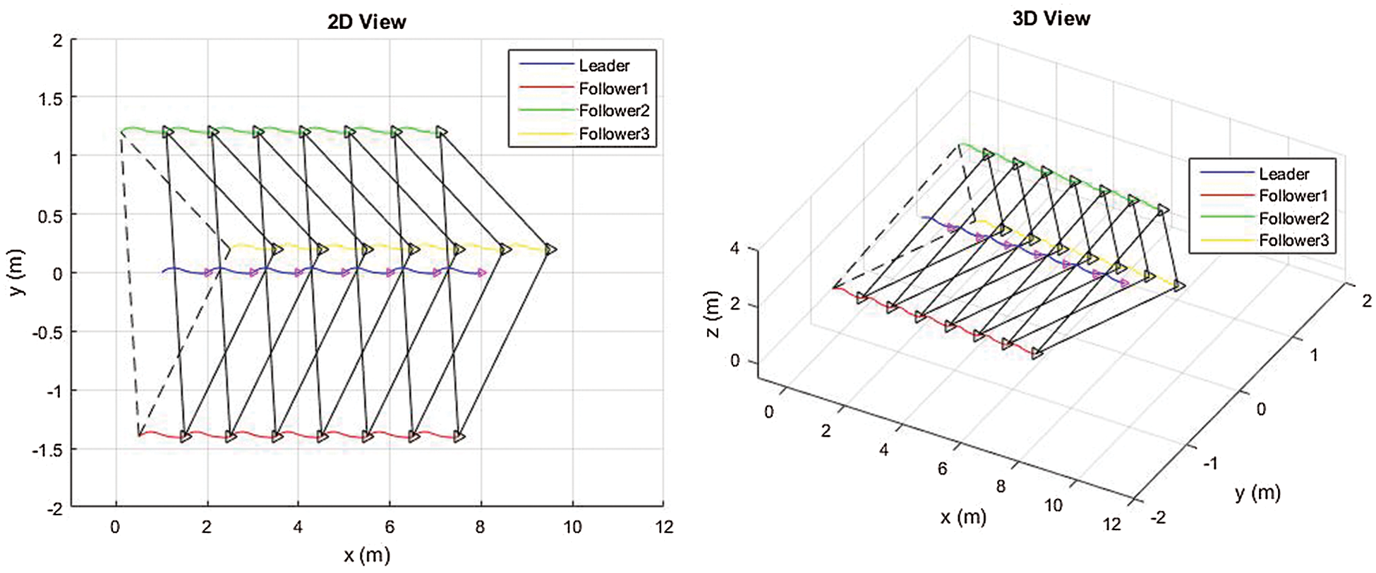
Figure 6: The group movement along the full path (different views)
The leader and follower quadrotors are first set to their initial hovering positions. The leader then moves in x-y direction, and the followers follow the leader while keeping the desired formation. The initial position of the leader is taken as (1,0,2) and that of the followers as (0.5,−1.4,2), (0.1,1.2,2) and (2.5,0.2,2), respectively, for each follower. The leader’s final position is then set to (7,6,2), where the motion is in steps of 1. The simulation results can be seen in Fig. 7.
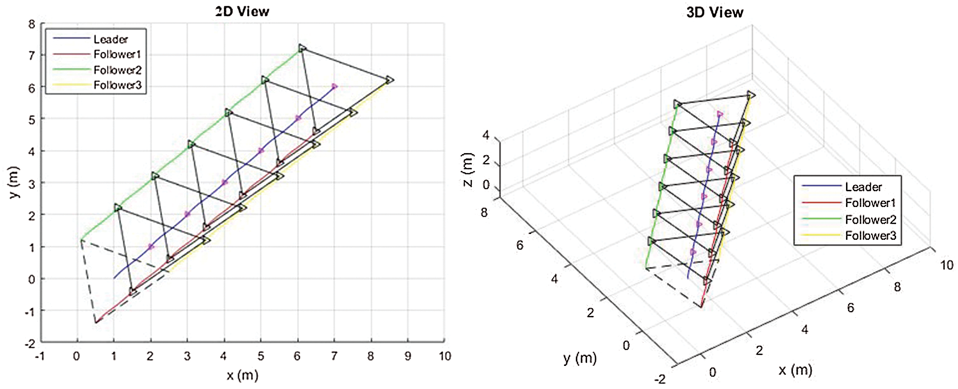
Figure 7: The group movement along the full x-y path (different views)
The leader and follower quadrotors are first set to their initial hovering positions. The leader then moves linearly in the x-y-z plane, and the followers follow the leader while keeping the desired formation. The initial position of the leader is taken as (1,0,2) and that of the followers as (2.2,0.8,1.8), (−0.3,0.7,2.1) and (1,−1.5,1.7), respectively, for each follower to form a 3D polygon. The leader’s final position is then set to (7,6,8), where the motion is in steps of 1. The simulation results can be seen in Fig. 8.
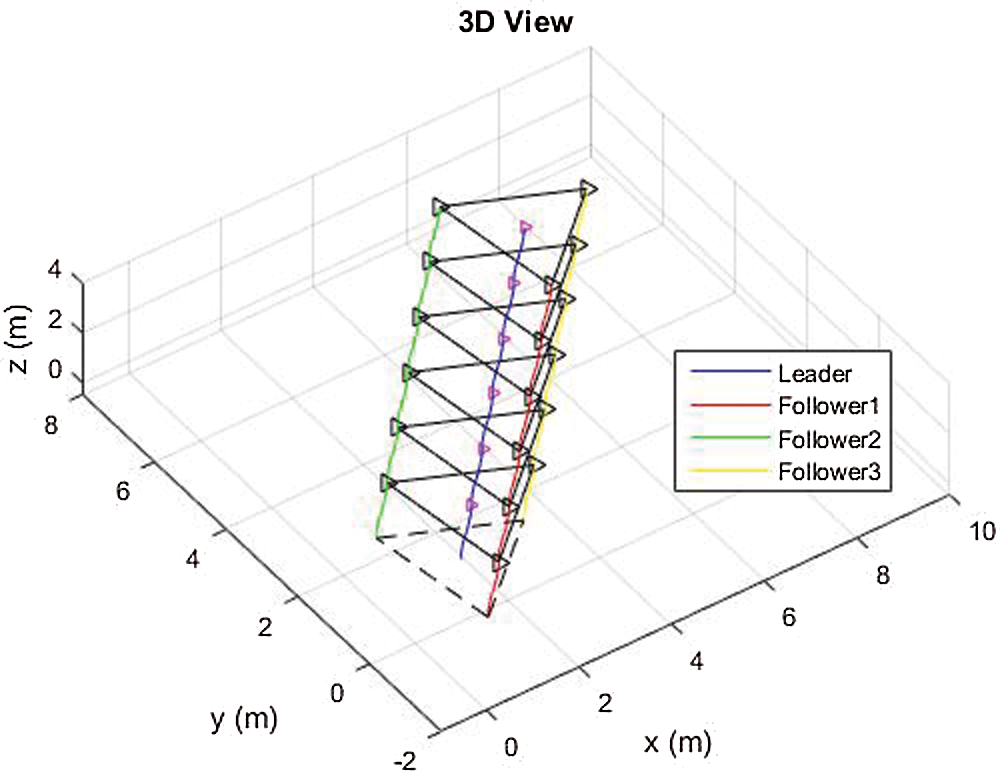
Figure 8: The group movement along the full x-y-z path
The leader and follower quadrotors are first set to their initial hovering positions. The leader is then set to move in a sinusoidal path, and the followers follow the leader while keeping the desired formation. The initial position of the leader is taken as (1,0,2) and that of the followers as (2.2,0.8,1.8), (−0.3,0.7,2.1), and (1,−1.5,1.7), respectively, for each follower to form a 3D polygon. The leader then moves in the form of a sinusoidal trajectory, which is the form of  for each coordinate x, y, and z. The different views of the simulation results can be seen in Figs. 9–12.
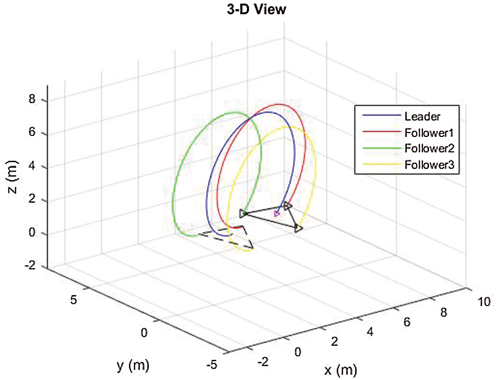
Figure 9: 3D view of the group movement for a sinusoidal reference trajectory
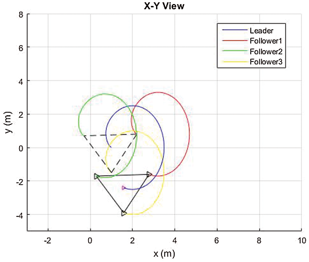
Figure 10: x-y view of the group movement for a sinusoidal reference trajectory
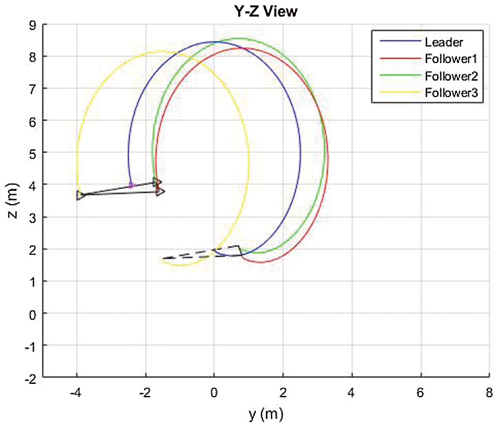
Figure 11: y-z view of the group movement for a sinusoidal reference trajectory
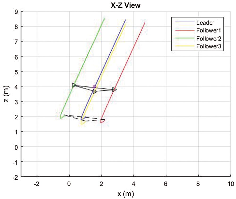
Figure 12: x-z view of the group movement for a sinusoidal reference trajectory
Figs. 9–12 show the different views of the complete trajectory of the group of quadrotors for the sinusoidal motion. From the results, we see that we can obtain the desired tracking and formation responses.
Therefore, from all the simulation results, it can be concluded that the proposed formation control scheme works efficiently with the nonlinear model of the quadrotor. It provides a smooth tracking of the group of quadrotors for a detheired formation flight.
In this paper, a cooperative flight control framework is designed for a fleet of an arbitrary number of UAVs. Our approach’s novelty is in considering the difference between the nonlinear model and the linearized ones as disturbance. These local linear models are then interpolated using the Gaussian membership functions from fuzzy theory to approximate the entire nonlinear model. Then a nonlinear state-feedback controller is synthesized using the PDC. The controller gains are obtained by the LQR optimization to stabilize the system and obtain the desired response. This is then followed by the formation control of a set of quadrotors using the leader–follower method. The potential field technique is used to obtain the desired shape formation. An attractive potential is generated to attract the followers towards the leader, and a repulsive potential is generated to repel adjacent quadrotors to avoid collisions. Simulations are performed to obtain the desired shape formation for different cases. It is observed that the new method of linearization and the formation control proposed gives a good tracking response, and we can achieve the required formation. The obtained results are smoother than those reported in Saif et al. [4].
Funding Statement: The authors would like to thank the DSR at KFUPM (https://dsr.kfupm.edu.sa/) for the support received under project numbers IN141048 and DF191006.
Conflicts of Interest: The authors declare that they have no conflicts of interest to report regarding the present study.
1. S. Bouabdallah, “Design and control of quad rotors with application to autonomous flying,” Ph.D. dissertation, ingénieur d’état, Université Aboubekr Belkaid, Tlemcen, Algérie, 2007. [Google Scholar]
2. T. Takagi and M. Sugeno. (1985). “Fuzzy identification of systems and its applications to modeling and control,” IEEE Transactions on Systems, Man, and Cybernetics, vol. SMC-15, no. 1, pp. 116–132. [Google Scholar]
3. M. Najib and H. Al-Absari. (2016). “LQR formation control with collision avoidance of multiple quadrotors,” MSc thesis. King Fahd University of Petroleum & Minerals. [Google Scholar]
4. A. W. A. Saif, N. M. Al-Absari, S. El Ferik and M. Elshafei. (2020). “Formation control of quadrotors via potential field and geometric techniques,” International Journal of Advanced and Applied Sciences, vol. 7, no. 6, pp. 82–96. [Google Scholar]
5. S. Bouabdallah and R. Siegwart. (2007). “Full control of a quadrotor,” in Proc. IEEE/RSJ Int. Conf. Intelligent Robots and Systems, San Diego, USA, pp. 153–158. [Google Scholar]
6. I. Fantoni, R. Lozano and P. Castillo. (2002). “A simple stabilization algorithm for the PVTOL aircraft,” in Proc. 15th IFAC World Congress, Barcelona, Spain, pp. 1225. [Google Scholar]
7. A. Sanchez, I. Fantoni, R. Lozano and J. D. L. Morales. (2005). “Observer-based control of a PVTOL aircraft,” in Proc. 16th IFAC World Congress, Prague, Czech Republic, pp. 1980. [Google Scholar]
8. G. Jithu and P. R. Jayasree. (2016). “Quadrotor modelling and control,” in Int. Conf. on Electrical, Electronics, and Optimization Techniques (ICEEOTChennai, India. [Google Scholar]
9. R. Xu and U. Özgüner. (2008). “Sliding mode control of a class of underactuated systems,” Automatica, vol. 44, no. 1, pp. 233–241. [Google Scholar]
10. V. Mistler, A. Benallegue and N. K. M’sirdi. (2001). “Exact linearization and noninteracting control of a 4 rotors helicopter via dynamic feedback,” in 10th IEEE International Workshop on Robot and Human Interactive Communication, Bordeaux, Paris, France, pp. 586–593. [Google Scholar]
11. H. Voos. (2009). “Nonlinear control of a quadrotor micro-uav using feedback-linearization,” in Mechatronics, IEEE Int. Conf, Malaga, Spain, pp. 1–6. [Google Scholar]
12. E. Altug, J. P. Ostrowski and R. Mahony. (2002). “Control of a quadrotor helicopter using visual feedback,” IEEE Int. Conf. on Robotics and Automation, vol. 1, pp. 72–77. [Google Scholar]
13. Z. Zuo. (2010). “Trajectory tracking control design with command-filtered compensation for a quadrotor,” Control Theory & Applications, vol. 4, no. 11, pp. 2343–2355. [Google Scholar]
14. R. Xu and U. Ozguner. (2006). “Sliding mode control of a quadrotor helicopter,” in 45th IEEE Conf. on Decision and Control, San Diego, CA, USA, pp. 4957–4962. [Google Scholar]
15. H. Bouadi, M. Bouchoucha and M. Tadjine. (2007). “Sliding mode control based on backstepping approach for an UAV type-quadrotor,” International Journal of Applied Mathematics and Computer Sciences, vol. 4, no. 1, pp. 12–17. [Google Scholar]
16. A. Tayebi and S. McGilvray. (2004). “Attitude stabilization of a four-rotor aerial robot,” 43rd IEEE Conf. on Decision and Control, vol. 2, pp. 1216–1221. [Google Scholar]
17. F. Yacef. (2011). “Réseau de modèles locaux pour la commande d’un UAV de type quadrotor,” dissertation. University of Jijel, Algeria (in French). [Google Scholar]
18. S. Latyshev. (2013). “Flexible formation configuration for terrain following flight: Formation keeping constraints,” Los Angeles, USA. [Google Scholar]
19. L. Di. (2011). “Cognitive formation flight in multi-unmanned aerial vehicle-based personal remote sensing systems,” Utah State University, Logan, USA. [Google Scholar]
20. Y. Zhang and H. Mehrjerdi. (2013). “A survey on multiple unmanned vehicles formation control and coordination: normal and fault situations,” in Int. Conf. on Unmanned Aircraft Systems (ICUASAtlanta, GA, USA. [Google Scholar]
21. I. S. Choi and J. S. Choi. (2012). “Leader-follower formation control using PID controller,” in 5th Int. Conf. on Intelligent Robotics and Applications, Montreal, Canada, pp. 625–634. [Google Scholar]
22. J. D. Wolfe, D. F. Chichka and J. L. Speyer. (1996). “Decentralized controllers for unmanned aerial vehicle formation flight.” San Diego, USA. [Google Scholar]
23. J. A. Guerrero and R. Lozano. (2010). “Flight formation of multiple mini rotorcraft based on nested saturations,” in IEEE/RSJ Int. Conf. on Intelligent Robots and Systems (IROSTaipei, Taiwan. [Google Scholar]
24. M. Turpin, N. Michael and V. Kumar. (2012). “Decentralized formation control with variable shapes for aerial robots,” in 2012 IEEE Int. Conf. on Robotics and Automation (ICRASaint Paul, MN, USA. [Google Scholar]
25. C. J. Ru, R. X. Wei, Y. Y. Wang and J. Che, “Multimodel predictive control approach for UAV formation flight,” Hindawi Publishing Corporation, Mathematical Problems in Engineering, London, United Kingdom, 2014, [Google Scholar]
 | This work is licensed under a Creative Commons Attribution 4.0 International License, which permits unrestricted use, distribution, and reproduction in any medium, provided the original work is properly cited. |