DOI:10.32604/iasc.2021.015227
| Intelligent Automation & Soft Computing DOI:10.32604/iasc.2021.015227 | |
| Article |
Automatic BIM Indoor Modelling from Unstructured Point Clouds Using a Convolutional Neural Network
Department of Computer Science and Engineering, Seoul National University of Science and Technology, Seoul, Korea
*Corresponding Author: Ji-Hyeong Han. Email: jhhan@seoultech.ac.kr
Received: 11 November 2020; Accepted: 03 February 2021
Abstract: The automated reconstruction of building information modeling (BIM) objects from unstructured point cloud data for indoor as-built modeling is still a challenging task and the subject of much ongoing research. The most important part of the process is to detect the wall geometry clearly. A popular method is first to segment and classify point clouds, after which the identified segments should be clustered according to their corresponding objects, such as walls and clutter. To perform this process, a major problem is low-quality point clouds that are noisy, cluttered and that contain missing parts in the data. Moreover, the size of the data introduces significant computational challenges. In this paper, we propose a fully automated and efficient method to reconstruct as-built BIM objects. First, we propose an input point cloud preprocessing method for reconstruction accuracy and efficiency. It consists of a simplification step and an upsampling step. In the simplification step, the input point clouds are simplified to denoise and remove certain outliers without changing the innate structure or orientation information. In the upsampling step, the new points are generated for the simplified point clouds to fill missing parts in the plane and nearby edges. Second, a 2D depth image is generated based on the preprocessed point clouds after which we apply a convolutional neural network (CNN) to detect the wall topology. Moreover, we detect doors in each detected wall using a proposed template matching algorithm. Finally, the BIM object is reconstructed with the detected walls and doors geometry by creating IfcWallStrandardCase and IfcDoor objects in the IFC4 standard. Experiments based on residual house point cloud datasets prove that the proposed method is reliable for wall and door reconstruction from unstructured point clouds. As a result, with the detected walls and doors, 95% of the data is successfully identified.
Keywords: Building information modeling (BIM); point cloud; LiDAR; convolutional neural network (CNN)
The automated reconstruction of building information modeling (BIM) models is becoming increasingly widespread in the architectural, engineering and construction (AEC) industry. At present, most existing buildings are not maintained, refurbished or deconstructed with BIM [1,2]. BIM modelling in existing buildings is significant, especially for restoration, heritage documentation, maintenance, quality control and project planning. Moreover, the existing documentation of a building often does not match the as-design model of the building due to construction changes or renovations [3,4] The implementation of as-built BIM models faces several challenges. For instance, information about the structural elements of buildings is often sparse or non-existing due to scanner errors. The common procedure of the BIM model consists of steps that describe the geometric structure of the building elements and reconstructs the described elements in the BIM structure.
Currently, the scan-to-BIM process is mainly a labor-intensive manual process performed by modelers. It uses a large number of unstructured point clouds as the input and manually designs all of the related objects in the scene. This is a time-consuming procedure and thus automated methods have been presented to speed up the process. We focus on the geometry of wall objects, which describe the basis of the building structure and can be reliably identified in the input data.
Wall geometry methods focus on an unsupervised process from the input data. The interpretation of this data is challenging due to the number of points, noise, clutter and the complexity of the structure [5]. Moreover, most point clouds are acquired by a laser scanner, and the common technique used in building surveying is terrestrial laser scanning (TLS). In the resulting data, some important parts of the structure are missing and occluded due to scanner errors and clutter. The method proposed in this paper deals with these problems with a preprocessing step. These problems are often improved by integrating the sensor’s position and orientation. However, our goal here is to work on sensor-independent data while considering the inputs as unstructured. The emphasis of this work is to take large unstructured point clouds of buildings as the input for the reconstruction of walls and their corresponding doors. More specifically, we propose a big-data preprocessing mechanism with simplification and upsampling steps. In the simplification step, we reduce input point clouds that denoise and remove some outliers without changing the innate structure or the orientation information. In the upsampling step, we solve the problem of missing parts in the data. We apply a 2D CNN method to detect the wall topology, and this step provides more accurate results than other methods. The proposed method is able to reconstruct and define wall topologies correctly even in highly cluttered and noisy environments. In addition to wall detection, we propose a method that detects doors in the detected walls to construct the BIM model. The main contributions of the proposed method are as follows:
• The proposed framework is fully automated. It takes only unstructured 3D point clouds collected by a laser scanner as the input, and the output is a reconstruction of BIM objects in the IFC format. The output can be edited in CAD (computer-aided design) programs.
• An efficient and accelerated preprocessing step that improves the accuracy of the wall geometry is proposed. As a result, we generate a depth 2D image with clear wall candidate lines.
• We apply a state-of-the-art wireframe parsing network (L-CNN) for detecting wall topologies. It is best suited for room and wall boundary detection from a 2D image.
• A door detection method in the corresponding walls is also proposed.
This paper is organized as follows. In Section 2, the background and related work are presented. Section 3 presents the proposed method, including the steps of data preprocessing, wall detection, door detection and BIM reconstruction. In Section 4, experimental results and the implementation process are discussed, including the evaluation metrics and datasets used. Finally, the concluding remarks follow in Section 5.
Automated BIM modelling from point clouds is a popular topic related to buildings. The most important part of the BIM structure is the geometry of the wall objects, which describe the basis of the building structure. Many different approaches and algorithms have been studied for several years in an effort to define the wall geometry from point clouds, and these methods have several procedures in common [6]. First, data preprocessing is performed to create more structured data in order to reduce the processing time and achieve more efficient results. In 2D methods, the initial point cloud is represented as a set of 2D raster images by slicing the data or by projecting the points onto a plane [7,8]. In 3D methods, the initial point cloud is regularized and compressed by an octree structure [9]. In both methods, the point cloud is segmented subsequently. Typically, line segmentation methods are used in 2D methods such as RANSAC based [7,10–12] and Hough transform based [13–15] methods, while plane segmentation methods are used in 3D methods [9,16–18]. RANSAC [19] is not only the line segmentation method but also the most popular plane segmentation method. The basic RANSAC algorithm incurs a high computational cost when used with very large point clouds. To find the largest plane, it checks all possible plane candidates in the input data. Schnabel et al. proposed an efficient RANSAC algorithm that checks plane candidates in subsets of the input data [20]. The plane candidates are defined until the probability of the largest candidate is lower than a user defined threshold. The largest plane is continually detected until there are no additional planes, with this action limited to covering the user-defined threshold [20]. Then, the point cloud is classified. Each extracted segment is processed by a reasoning algorithm that computes class labels such as walls, floors and ceilings for each observation. The input data is described by a set of numeric values that encodes the corresponding characteristics. Typically, these features represent distinct geometric and contextual information [21,22]. The classification algorithms that process the feature vectors use either heuristics or more complex classification methods such as random forests (RF), neural networks (NN), probabilistic graphical models (PGM), and support vector machines (SVM) [23–27]. Moreover, convolutional neural networks and conditional random fields (CRF) are presented for the classification of the BIM geometry [28,29]. Finally, reconstruction algorithms create the correct BIM geometry for each class based on the labelled dataset. This includes the associative clustering of the labelled points or segments to encompass a single object. The individual components of the object are also identified, e.g., the clusters that compose a single wall face of a wall. Once the input data is interpreted, the necessary metric information is extracted to compute the object position, orientation and dimensions. Several studies have attempted to reconstruct wall geometries using machine learning techniques. Xiong et al. and Adan and Huber used machine learning to reconstruct planar wall boundaries and openings [23,30]. Michailidis and Pajarola used Bayesian graph-cut optimization with cell complex decomposition to reconstruct highly occluded wall surfaces [31].
During the preprocessing step, most existing methods use point cloud filtering algorithms in order to remove noise and outliers, separately, such as a pass-through filter, a statistical outlier removal filter, or a voxel grid filter. These algorithms reduce the amount of data and remove outliers, but they may miss and change critical geometric features such as the position and the orientation. Point cloud simplification algorithms are able to replace the aforementioned algorithms in both 2D and 3D methods. Moreover, only one simplification algorithm can solve both noise and outlier problems. Many algorithms for the simplification of point clouds have been introduced [32]. The grid-based simplification algorithm is more efficient than other algorithms. However, it has a data quality problem when used with reduced data. Pauly et al. proposed hierarchical and incremental clustering algorithms to create approximations of point-based models. This involves data sampling to generate points of lower density [33]. However, some critical geometric features can be missed upon any division. Lipman et al. [34] introduced the locally optimal projection (LOP) operator, which is a parameterization-free projection operator, motivated by the concept of the L1 median [35,36]. The concept of their method is that the subset of the input point cloud is repeatedly projected onto the corresponding point cloud in order to reduce outliers and noise. However, this creates non-uniform data, and if the input data is highly non-uniform, problems will arise when estimating normal and projecting shape features. Huang et al. [37] solved this problem by introducing weighted locally optimal projection (WLOP), which creates a more distributed point cloud incorporating the locally adaptive density weights of each point into the LOP.
The automated BIM process also faces the problem of a lack of information in the data. Point cloud upsampling methods are used to address this problem. Jones et al. and Oztireli et al. [38,39] proposed a bilateral normal smoothing method that smooths the input data by repeatedly projecting each point onto an implicit surface patch fitted over its nearest neighbors. Bilateral projection preserves sharp features according to the normal (gradient) information. Normals are thus required as the input. However, this method can nonetheless produce erroneous normals near the edges. Huang et al. proposed an edge-aware solution with two different projection operators. The first introduced a robust edge-aware projection operator that creates a sample away from the edges. The second was a novel bilateral projection operator that up-samples repeatedly to fill the edge regions [40].
The line segmentation step is a key aspect of 2D methods, and it highly depends on the quality of the generated 2D image. Currently, traditional methods are utilized and perform well, with examples being such as RANSAC [20], the Hough transform [41], the least-square (LS) method [42], and the efficient line detection method [43]. Also, deep learning-based methods outperform when starting with images; specifically, the wireframe parsing method is well suited for detecting wall topologies. Previous studies [44,45] solved the wireframe parsing problem in two steps. First, a deep CNN generated pixel-wise junctions and line heat maps from 2D images. Then, junction positions, line candidates, and the corresponding connections were defined using a heuristic algorithm based on the generated heat map. These types of studies have been widely used in line detection problems; however, the vectorization algorithm in this line of research is highly complex and depends on heuristic solutions. Moreover, it occasionally produces inferior solutions. Zhou et al. proposed a new end-to-end wireframe parsing solution called L-CNN that uses a single and unified neural network [46].
The detection of openings is also challenging in the area of building reconstruction. This mainly focuses on building facades. Facades structures have specific characteristics, which include regularity, orthogonality and regular patterns. Typically, the methods that rely on these characteristics must address the issue of missing parts in facades. Böhm [47] proposed a method to complete missing parts in point clouds acquired by terrestrial laser scanning, accomplished by repeatedly using the repetitive information often present in urban buildings. Zheng et al. introduced another method with a similar goal, proposing a method for completing holes in scans of building facades. Their method utilizes iteration to consolidate incomplete data [48]. Previtali et al. proposed a method based on lattice schema. They assume that elements on building facades are distributed in an irregular lattice schema. The lattice candidates are defined using a voting scheme and the final lattice is defined by minimizing a score function [49].
The final step of BIM reconstruction is to define the relationships between the elements in a building. Building elements are described by their topology. Topological data explain the element relationship information; therefore, the locations and dimensions of building elements are described based on geometrical information. Several researchers have proposed automatic methods for determining topological relationships between objects. Nguyen et al. [50] proposed a method that analyzed the topological relationships between building objects automatically. Belsky et al. [51] introduced a prototype system that attempted to improve upon prior model files. They used geometric, topological, and other main operators in collections of rule sets. Anagnostopoulos et al. proposed a semi-automatic method that estimated the boundaries and adjacency of building objects in point cloud data and produced reconstructed building objects in the IFC format as the output [52].
In this section, we present our implementation of the proposed method. The proposed method takes unstructured point clouds as the input, with the output being a set of walls with corresponding doors according to the as-built conditions of the building. We implemented our method in three steps. First, the input data is preprocessed for efficiency and reliability of the algorithm, consisting of simplification and upsampling steps. The simplification step reduces the number of points for efficiency, after which the upsampling step fills in missing points on planes and at nearby edges for reliability. Second, the walls are detected based on preprocessed point cloud using a 2D CNN method. Moreover, we detect doors in each detected wall using a template matching method. Finally, BIM objects are reconstructed using the information from the detected walls and doors. The proposed method is fully automated and implemented using C++. Fig. 1 shows the overall flow of the proposed method. The details of each step are explained in the following subsections.
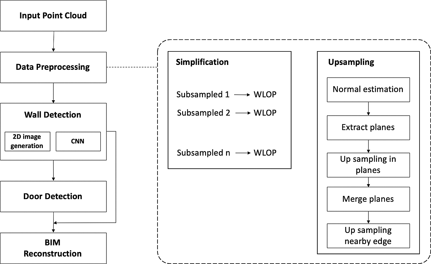
Figure 1: Overview of the proposed method that automatically creates BIM objects from unstructured point clouds
The input data are large unstructured point clouds collected by a laser scanner that contain noise, outliers, and non-uniformities in the thickness and spacing due to acquisition errors or misalignments of multiple scans. Therefore, the input point cloud must be preprocessed which has a crucial impact on the final results. The output of this step is downsampled 3D point cloud, which is clearer and more distributed. Two types of algorithms are utilized in this step: simplification and upsampling.
3.1.1 Simplification (Downsampling)
For input data downsampling, we use a point cloud simplification algorithm called WLOP instead of a traditional point cloud filtering algorithm. WLOP not only simplifies the input data but also regularizes the downsampled input point clouds, i.e., by denoising, outlier removal, thinning, orientation, and with a redistribution of the input point clouds. Point cloud simplification aims to find a point cloud X with a target sampling rate that minimizes the distance between the surfaces, as represented by X and the input point cloud P.
WLOP takes unstructured point clouds
where
The WLOP reduces the input points according to Eq. (1) without changing the innate structure or orientation information; however, it introduces a computational cost problem. Thus, we propose an accelerated WLOP algorithm that incurs a lower computational cost than the traditional WLOP algorithm. First, we sample subset points from input data using a height histogram. Subsequently, we apply WLOP to each sampled subset. According to our experiments, WLOP requires less than 28 seconds for fewer than 200,000 points. If there are more than 200,000 sub-sampled points, we decrease the bin size until each subset has fewer than 200,000 points. This speed-up method decreases the computational time of traditional WLOP at least 2.5 times.
After the input data simplification process, we obtain the simplified 3D point cloud with less noise and fewer outliers, with a more distributed point cloud as well. However, the remaining 3D point clouds still have missing parts. In order to solve this problem, we propose two up-sampling methods. The first fill holes in the planes via the following steps:
• Take the simplified 3D point cloud as the input and estimate the normal from the input data using a basic principal component analysis (PCA). Using Eq. (2), the covariance matrix K with the nearest neighbor k is calculated. Using Eq. (3), the plane-normal direction is estimated using the minimum eigenvector in that set of neighbors. It only estimates unsigned normal directions, which may be unreliable due to a thick point cloud and a non-uniform distribution.
• The estimated normals are oriented using the method proposed by Hoppe et al. [53].
• To extract all possible wall candidate planes based on 3D point cloud with oriented normals, the efficient RANSAC approach is used with a regularization method that regularizes planes to make them parallel and orthogonal.
• Finally, we obtain several wall candidates planes with distributed points. We calculate the bounding boxes of each detected wall candidate plane and search for missing parts in the corresponding bounding box. Then, new points are generated to fill in the corresponding missing parts; several examples of this are presented in Fig. 2. Therefore, we need to check for doors in each wall using Algorithm 1 while filling in missing parts on the planes. If a missing part is detected as a door, it is not filled in with new points. The output of this step is 3D point cloud with the missing parts in the data filled in along with the oriented normal.
In these equations,
The second method is to fill in missing parts close to edges. We use an edge-aware up-sampling method introduced in earlier work [40]. The edge-aware up sampling method takes oriented 3D point cloud as the input and then determines how carefully to resample points close to edges with reliable data. To do this, a sequence of insertion operations is needed. During each insertion, the up-sampling method adds a new oriented point that fulfills three objectives:
• The corresponding point lies on the underlying surface.
• The corresponding normal is perpendicular to the underlying surface at the point.
• After insertion, the points are more distributed in the local neighborhood.
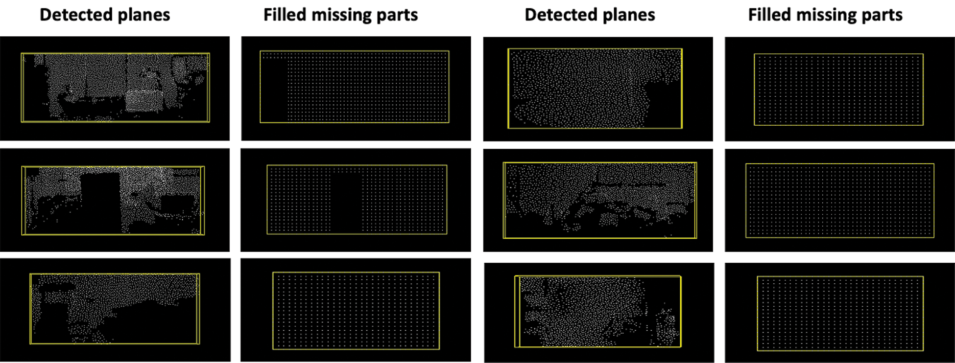
Figure 2: Example results of the filling in of missing parts in the detected plane: the yellow rectangle describes the bounding box of the detected plane
We merge all planes obtained in the previous steps into one-point clouds and then apply the edge-aware up-sampling method to fill in missing parts close to edges. Several examples are presented in Fig. 3. The output of this step is 3D point cloud with the missing parts in the data filled in.
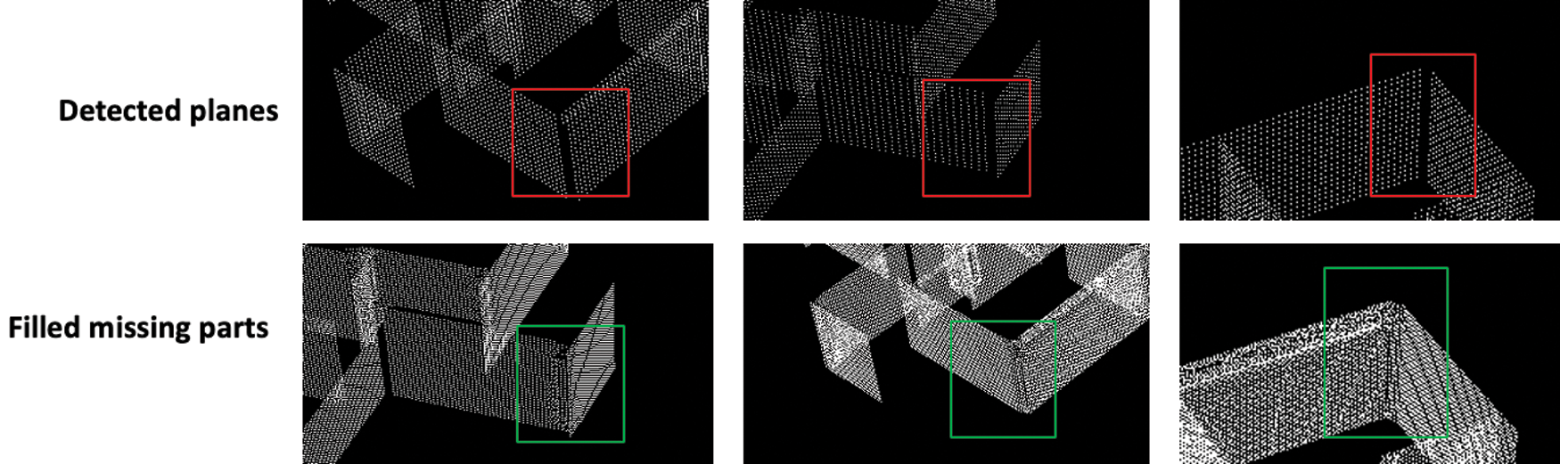
Figure 3: Example results of filling in missing parts close to edges: the red and green rectangles describe missing parts close to edges and the results after filling the points, respectively
After the preprocessing step, we have a more distributed and clearer 3D point cloud, which is the input of this step. We then generate a 2D image using a method in our previous work [43]. We remove remaining clutter from preprocessed point cloud when applying this method. Generally, the points at about 30cm on the ceiling contain clearer data in buildings. In other words, clutter is mostly absent at this level of points in buildings. Hence, we slice points at 30cm in the ceiling areas from the up-sampled point cloud. The sliced points are then projected onto the x-y plane, and we create a 2D depth image from the projected points. For wall topology detection, we use the L-CNN architecture, a type of CNN [46]. It takes a 2D image as the input and contains four modules that undertake the following:
• The shared intermediate feature maps are generated by a feature extraction backbone network that takes a 2D image as the input.
• The junction candidates are defined using a junction proposal module. Our generated image has clear edges due to the use of an edge-aware upsampling method.
• Line proposals are defined using the junction candidates by a line sampling module.
• The proposed lines are defined by a line verification module.
The final outputs of L-CNN are the positions of the junctions and a connection matrix between those junctions. Fig. 4 shows the overall flow of the L-CNN architecture.
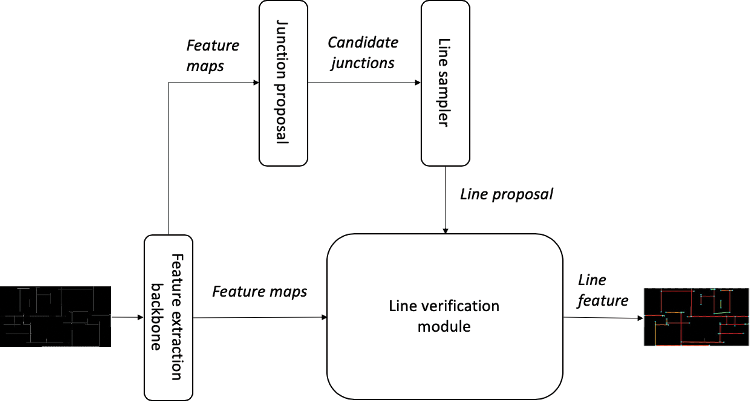
Figure 4: Overview of the L-CNN architecture for detecting wall topologies
After the wall detection step, we detect doors in the corresponding walls with Algorithm 1. Several examples are presented in Fig. 5. We use the detected wall information as the input of this step, and the output of this step is the detected door information. Door detection involves the detection of holes in the wall plane that are the sizes of doors. If the doors are half opened, we remove such points as clutter in the preprocessing step. When data is acquired using laser scanners, there are no door points left on the floor. Based on this information, we scan all doors with the determined door template in each wall. Instead of using Algorithm 1 for only one wall, we use this algorithm repeatedly with all detected walls. The algorithm works as follows:
• Inputs are wall points, which are the results from the L-CNN network and the thresholds, i.e., the maximum height of the door, maxHeight, and the maximum length of the wall line, maxWidth.
• Define the door candidates, doorprop (lines between 1 and 15 in Algorithm 1). First, the algorithm calculates a bounding box of given wall, c. Then, every possible door candidate is checked based on a predefined template according to the coordinates from (minz, minx) to (minz, maxx) with the step size denoted as step. In this algorithm, the door has a predefined template with the width, maxWidth, and height, maxHeight specified. As a result, we find all door candidates with information that contains the starting point and number of error points in the door.
• Define actual doors from door candidates, doors (lines between 16 and 22 in Algorithm 1). First, the algorithm calculates the minimum number of error points, doorpoints, using the maximum error points of the detected doors, maxpoints, and a constant ratio of error points of per door, perdoorpoints. Then, all door candidates are checked, and if a candidate door has fewer error points than doorpoints, it is detected as a door.
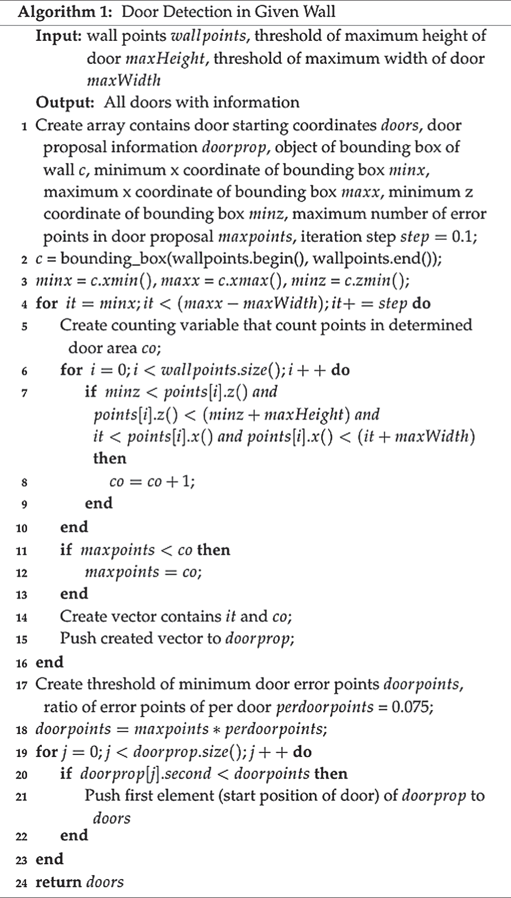
Algorithm 1: Door Detection for a Given Wall
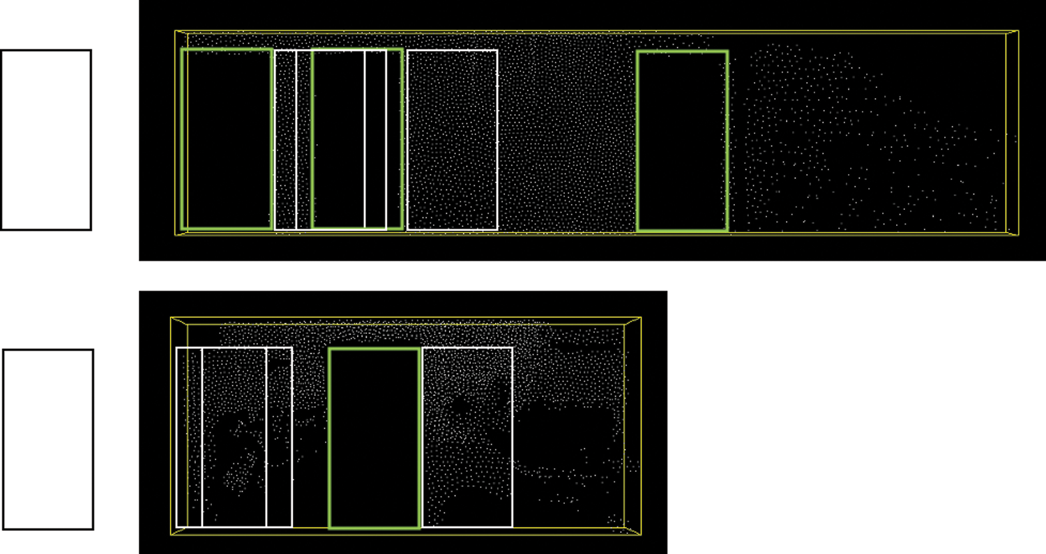
Figure 5: Example results of door detection: the black rectangles are door templates, the white rectangles show the iteration of the door template matching method, and the green rectangles describe detected doors
The walls and doors are detected successfully with their positions, directions and altitudes by the proposed method. However, they are still in the form of point clouds. The final step is to create actual BIM objects based on the detected elements. A conversion phase is thus necessary to be able to integrate the results into the BIM software. We chose the IFC format as the format for the output of our method. The IFC format is a standardized object-based file format used by the AEC industry to facilitate interoperability between building actors. In order to generate a file in the IFC format from a 3D geometry of structural elements, we used the open-source library IfcOpenShell [54].
The reconstruction step computes the necessary parameters for the creation of the BIM geometry. In this paper, generic IfcWallStandardCase entities are constructed based on the parameters extracted from the detected walls. The extracted parameters include the direction, thickness, position and boundary of the walls. As is common in manual modelling procedures, standard wall cases are created. This implies that the reconstructed walls are vertical, have a uniform thickness and have a height equal to the story height. The direction of the IfcWallStandardCase entities is derived from the detected wall lines. The wall plane normal is computed orthogonally to the direction of the wall lines. We use the default thickness based on our experimental result. The position is described as a line starting coordinate, and the boundary of wall is described as a line length. The generic IfcDoor entities are constructed based on the parameters extracted from the detected doors. The extracted parameters include the direction and position. The direction of the IfcDoor entities is identical to that of the wall. This position is described as a starting coordinate of the detected door. The output of this step is the computed BIM geometry of the detected walls and doors in the IFC file format.
The proposed method was experimentally tested on residential houses. We evaluated the quality of the wall and door geometry outcomes using the recall, precision and F1 score metrics. This section explains the experimental environment and the results.
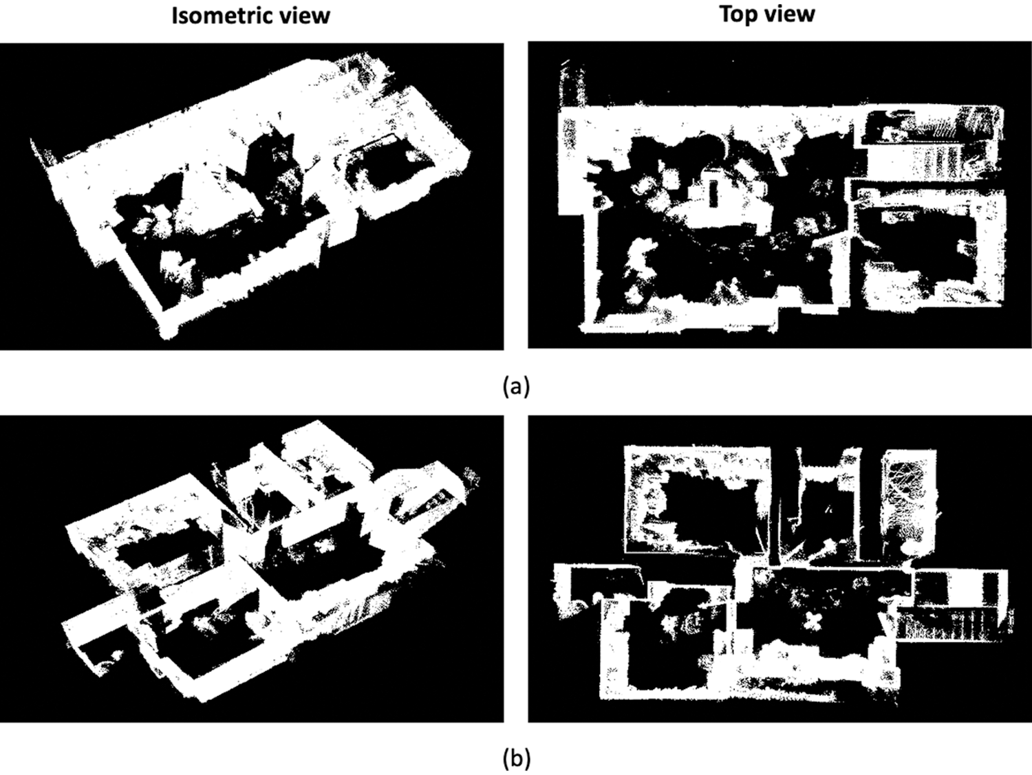
Figure 6: Input point clouds with two different views (isometric and top): (a) first floor of a residual house, and (b) second floor of a residual house
We developed the proposed method while focusing on data from the second floor of a residential house as collected by LIDAR (Velodyne HDL-32E) and tested the proposed method on the data of the first floor of the residential house collected by the same scanner to prove that the proposed method works robustly even for unseen data. This data is very noisy and contains numerous missing points in the walls, as it consists of multiple rooms with various types of clutter, such as desks, chairs, and sofas, as presented in Fig. 6. The proposed method used all of the point clouds as the input, as presented in Fig. 6. The first floor has 8,914,891 points and the second floor has 3,216,766 points. The details of each dataset are presented in Tab. 1. We decreased nearly 99.9% of the number of input point clouds, denoised the data, removed some outliers, and retrieved more structural data in the simplification step, as presented in Figs. 9a and 9c. Then, we up-sampled points in order to solve missing points in the downsampling step, as presented in Figs. 9b and 9d.
We defined thresholds based on our experiments. Fig. 7 shows the threshold settings for the second floor of the residual house. In detail, the percentage of points to store p and the neighbor size n_r are used in the WLOP algorithm. The sharpness of the result, a, the value used to determine how many points will be sampled near the edges, s, and the neighborhood size, e_r, are used in the edge-aware method. The minimum number of points for planes, min_points, and the maximum Euclidean distance between a point and a shape, e, are used in the efficient RANSAC. The point cloud grid size, grid_size, and the distance from the ceilings to the slice points, c_height, are used in the depth image generation algorithm. The line segmentation threshold, p, is used in the post process of the L-CNN. The maximum height of the door, max_height, the maximum width of the door, max_width, and the ratio of the error points per door, perdoorpoints, are used in the door detection step.
We evaluated the positions and lengths of the detected walls and doors by means of the precision, recall and F1 score, as used in pattern recognition, information retrieval and classification. The main concept of these methods is the fraction of relevant instances among the retrieved instances. We computed these metrics based on the overlap between the areas of the ground truth and the detected walls. We evaluated true-positive, false-positive and false-negative cases. True-positive (TP) refers to the area of a detected wall or door that is a wall or door in the ground truth, false-positive (FP) refers to the area of a detected wall or door that is not a wall or a door in the ground truth, and false-negative (FN) is the area that is a wall or a door in the ground truth but is not detected as a wall or a door by the proposed algorithm. The F1 score is the harmonic mean of the precision and recall, where an F1 score reaches its best value at 1 (perfect precision and recall). Based on TP, FP, and FN, we calculated the precision and recall as follows:
Moreover, based on precision and recall, we calculated the F1 score as follows:
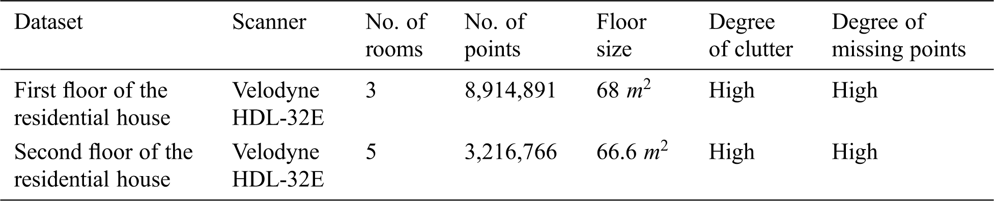
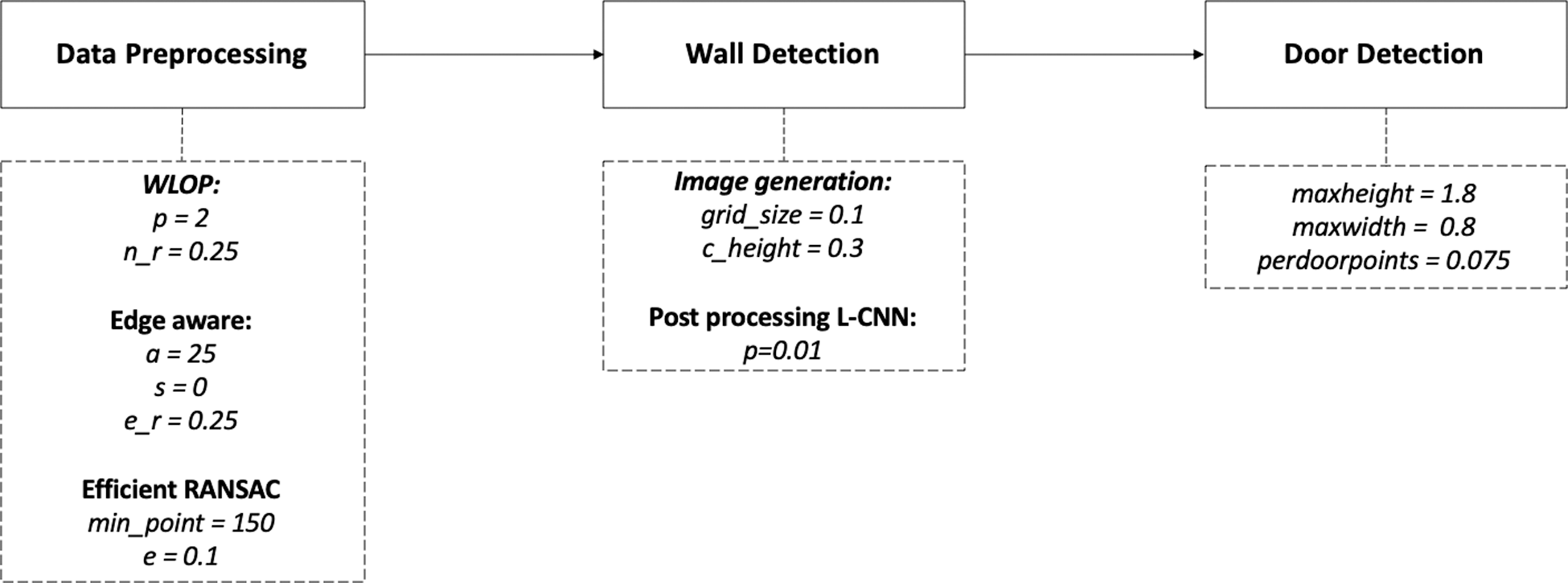
Figure 7: Thresholds used for the second floor of the residual house
We implemented the proposed method using C++, and the details of the algorithm used are presented in Fig. 8. The representative functions in the implementation are as follows:
• doSimplify() – The implementation of the simple WLOP algorithm. It works recursively.
• calcNormal() – Estimate the normal using the PCA.
• extract_planes() – Extract planes using the efficient RANSAC.
• doUpsampling() – Fill in missing parts in a plane and close to edges.
• generate2Dimage() – Generate a 2D depth image to detect the wall topologies.
• wallDetect() – Detect walls using the L-CNN network.
• doorDetect() – Detect doors in each of the detected walls.
• reconstructToBIM() – Create the BIM geometry from the 3D point cloud in the IFC file format.
The algorithm details are explained in Section 3 and threshold used are described in Section 4.1.
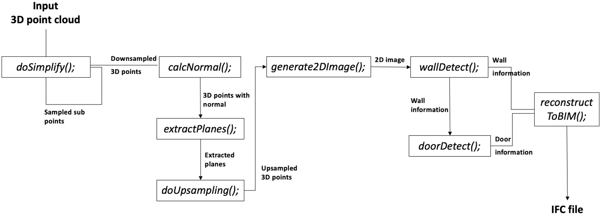
Figure 8: The overall process of the proposed method
During the overall wall detection process, we initially preprocessed the input data in two steps. First, we reduced input points using the proposed speed-up WLOP method. Figs. 9a and 9c show simplified point clouds of the first and the second floor of a residual house, respectively. Moreover, we compared the proposed speed-up WLOP method and the traditional WLOP method in terms of the computational impact using data of the residual house with different point densities, in this case data with 600K points, 2M points, 3.2M points, 8.9M points and 14.9M points. Tab. 2 shows the results of the comparison of the two methods. The proposed speed-up WLOP performed nearly 2.5 times faster than the traditional WLOP. In this step, we used a height histogram with a bin size of 0.5. Second, we up-sampled the data using the edge-aware method for missing parts in the data. Figs. 9b and 9d show the upsampled point clouds of the first and the second floors of the residual house, respectively. This is suitable for the applied L-CNN wall topology detection method because junction detection is an important part of the L-CNN. Then, we generated a depth image from the preprocessed data, as presented in Figs. 10a and 10c. For wall detection, we used the L-CNN method. These results are shown in Figs. 10b and 10d. The L-CNN was trained based on the ShanghaiTech dataset [44], which contains 5,462 images of man-made environments with wireframe annotation for each image that includes the positions of the salient junctions V and lines E, with a stacked hourglass network [55] used as the backbone network. We stopped the training at 16 epochs as the validation loss no longer decreased. The proposed method is more efficient than existing algorithms such as the Hough transform method. We implemented the Hough line transform algorithm from the OpenCV library [56] with the corresponding defined thresholds for a comparison with the proposed method. Tab. 3 shows the comparison result of wall geometry detection and the processing time of wall line detection on the second floor of the residual house. The experiments were performed using a MacBook Pro with a Dual-Core Intel Core i5 and 8 GB of memory.
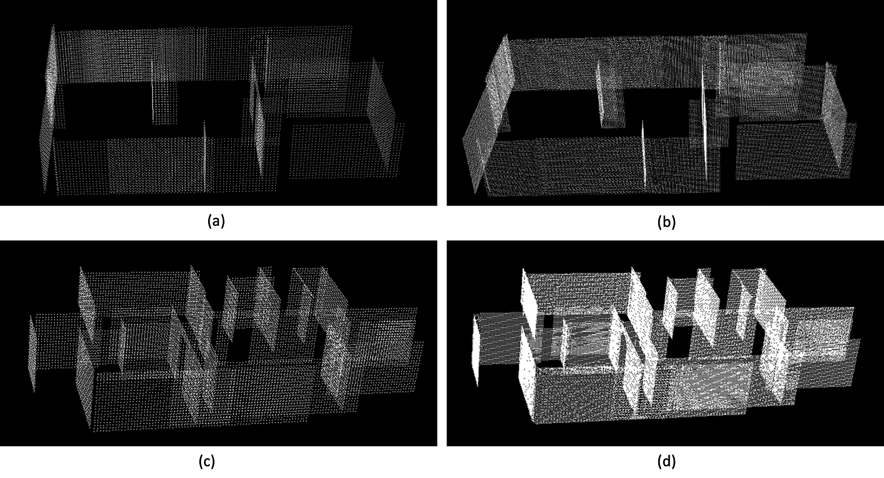
Figure 9: Result of the preprocessing step: (a) simplification result of the first floor, (b) upsampling result of the first floor, (c) simplification result of the second floor, and (d) upsampling result of the second floor
Fig. 11 shows the door detection result from the first and the second floors of the residual house. We successfully detected most of the doors in the input data. However, there are two limitations in our door detection results, as presented in Fig. 12. Because we removed door points as clutter in the preprocessing step based on the information that a door plane usually does not reached the ceiling level, the proposed door detection algorithm does not work with nearly closed or fully closed door, as presented in Fig. 12c. Also, the proposed algorithm does not work when there are numerous missing points around a door which are not recovered in usually up-sampling step, as presented in Fig. 12d.
Table 2: Computation Time Comparison of WLOP and the Proposed Speed-up WLOP
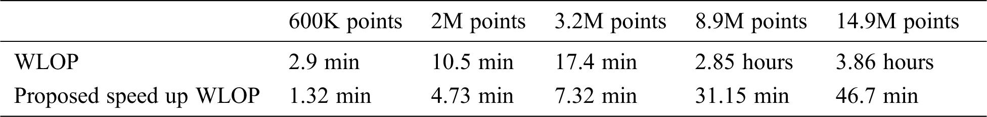
Table 3: Wall geometry detection and processing time comparison results of the hough transform-based method and the proposed method from experiments on the second floor of a residual house
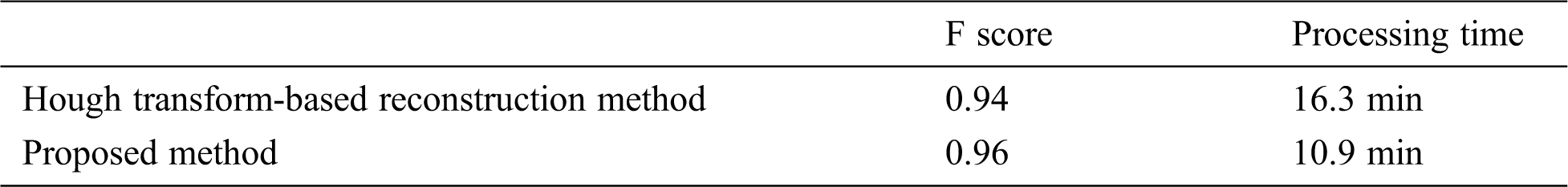
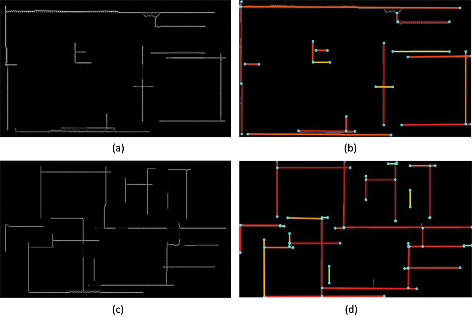
Figure 10: Result of wall detection: (a) depth image generation result of the first floor, (b) L-CNN wall topology generation result of the first floor, (c) depth image generation result of the second floor, and (d) L-CNN wall topology generation result of the second floor
Tab. 4 shows the final wall and door detection results. We detected 95% of the ground truth and reconstructed the detected walls and doors in the IFC file format, as shown in Fig. 13.
Table 4: Evaluation result of the proposed method
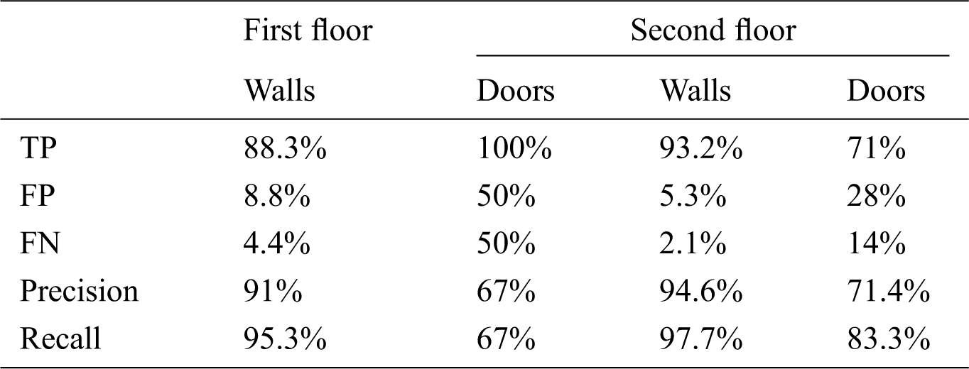
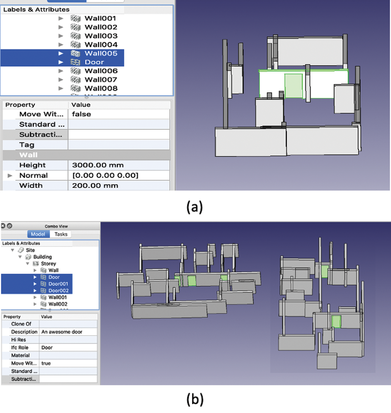
Figure 11: Results of door detection: (a) first floor and (b) second floor, where green shapes indicate detected doors
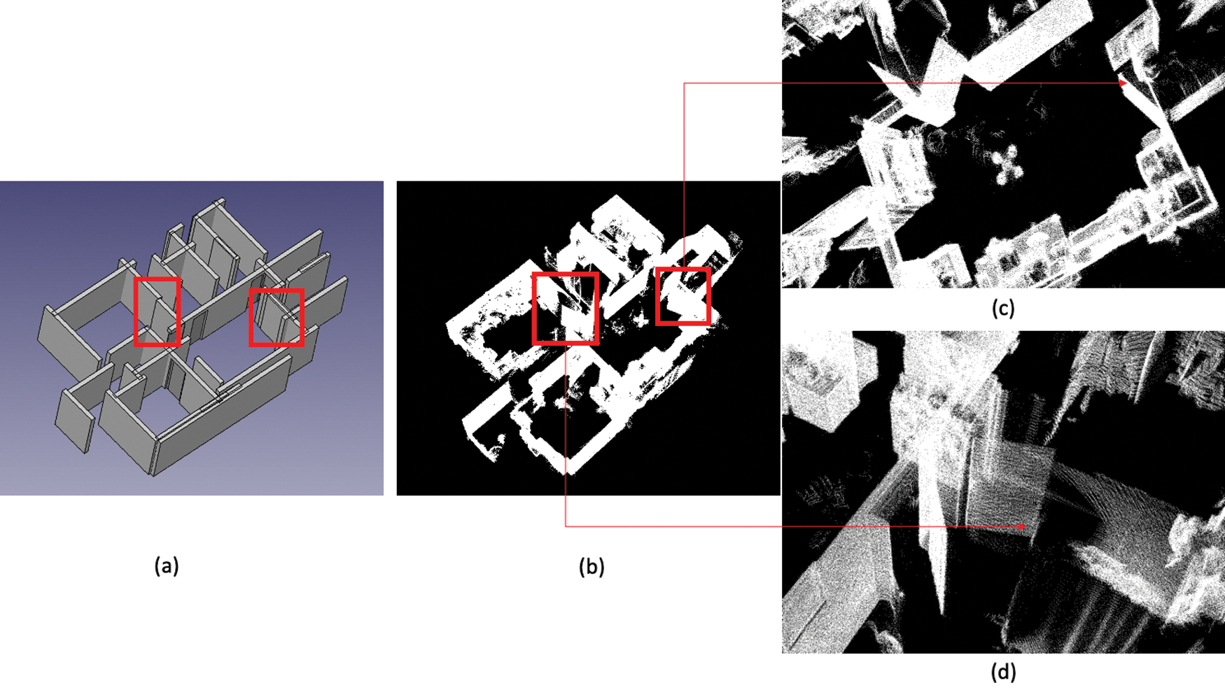
Figure 12: Failed results of door detection: (a) the result of the proposed method, (b) ground truth input data, (c) and (d) zoomed in failed cases. Red rectangles describe the positions of doors that were not detected
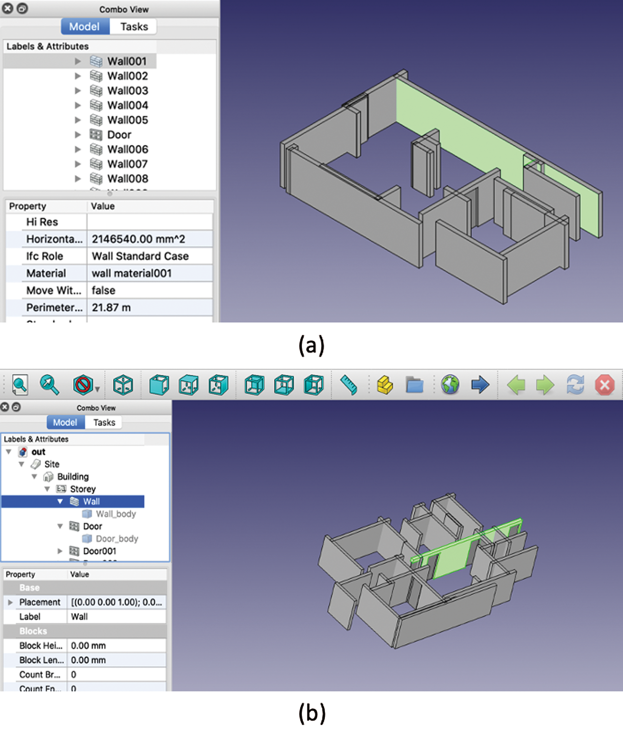
Figure 13: BIM results of proposed method: (a) first floor result and (b) second floor result
In this paper, we proposed a fully automated algorithm to reconstruct as-built BIM data from unstructured point clouds. First, we utilized the proposed big data preprocessing mechanism, which involved two steps. We proposed a speed-up WLOP algorithm in the simplification step and an edge-aware algorithm in the upsampling step. As a result of the proposed preprocessing method, we reduced the input data points with more distributed and structured data. The proper preprocessing of the unstructured input point clouds was the most significant step for wall topology detection to create the BIM. Second, the wall topology was detected using a 2D CNN, which is a L-CNN, and existing doors in each wall were detected by the proposed template matching algorithm. Finally, the proposed algorithm reconstructed detected walls in the BIM format, which can be edited in CAD programs. All of these steps are well suited to work with each of the other steps to improve the accuracy of the final results. For instance, after preprocessing the input data, we obtained a clear wall topology with clear edges. Therefore, this preprocessing result helped the most important part of the L-CNN architecture, which was to detect the junctions (edges) from the 2D image. We experimentally assessed the proposed algorithm on point cloud data gathered from the first and second floors of a residual house using LIDAR. More than 95% of the walls in the ground truth were detected, and the detected walls and doors were successfully generated in a BIM file. However, with regard to door detection, the proposed method had two limitations, i.e., when the doors are closed or almost closed, and there are numerous missing points around the doors. In the future, we will improve the door detection algorithm with a 2D CNN network and a more accurate generalization method.
Funding Statement: This work was supported by a grant from the National Research Foundation of Korea (NRF) funded by the Korean government (MSIT) (No. 2018R1A4A1026027).
Conflicts of Interest: The authors declare that they have no conflicts of interest to report regarding the present study.
1. R. Volk, J. Stengel and F. Schultmann. (2014). “Building information modeling (BIM) for existing buildings — literature review and future needs,” Automation in Construction, vol. 38, no. Part B3a, pp. 109–127. [Google Scholar]
2. R. Agarwal, S. Chandrasekaran and M. Sridhar. (2016). Imagining construction’s digital future. USA: McKinsey & Company. [Google Scholar]
3. I. Brilakis, M. Lourakis, R. Sacks, S. Savarese, S. Christodoulou et al. (2010). , “Toward automated generation of parametric BIMs based on hybrid video and laser scanning data,” Advanced Engineering Informatics, vol. 24, no. 4, pp. 456–465. [Google Scholar]
4. V. Patraucean, I. Armeni, M. Nahangi, J. Yeung, I. Brilakis et al. (2015). , “State of research in automatic as-built modelling,” Advanced Engineering Informatics, vol. 29, no. 2, pp. 162–171. [Google Scholar]
5. P. Tang, D. Huber, B. Akinci, R. Lipman and A. Lytle. (2010). “Automatic reconstruction of as-built building information models from laser-scanned point clouds: A review of related techniques,” Automation in Construction, vol. 19, no. 7, pp. 829–843. [Google Scholar]
6. A. Nguyen and B. Le. (2013). “3D point cloud segmentation: A survey,” in 2013 6th IEEE Conf. on Robotics, Automation and Mechatronics (RAMManila, Philippines, pp. 225–230. [Google Scholar]
7. I. Anagnostopoulos, V. Patraucean, I. Brilakis and P. Vela. (2016). “Detection of walls, floors and ceilings in point cloud data,” in Construction Research Congress, San Juan, Puerto Rico, pp. 2302–2311. [Google Scholar]
8. L. Landrieu, C. Mallet and M. Weinmann. (2017). “Comparison of belief propagation and graph-cut approaches for contextual classification of 3D lidar point cloud data,” in 2017 IEEE Intl. Geoscience and Remote Sensing Symposium, Fort Worth, TX, USA, pp. 2768–2771. [Google Scholar]
9. A. V. Vo, L. Truong-Hong, D. F. Laefer and M. Bertolotto. (2015). “Octree-based region growing for point cloud segmentation,” ISPRS Journal of Photogrammetry and Remote Sensing, vol. 104, no. 129, pp. 88–100. [Google Scholar]
10. S. Ochmann, R. Vock, R. Wessel, M. Tamke and R. Klein. (2014). “Automatic generation of structural building descriptions from 3D point cloud scans,” in 2014 Intl. Conf. on Computer Graphics Theory and Applications (GRAPPLisbon, Portugal, pp. 1–8. [Google Scholar]
11. C. Thomson and J. Boehm. (2015). “Automatic geometry generation from point clouds for BIM,” Remote Sensing, vol. 7, no. 9, pp. 11753–11775. [Google Scholar]
12. L. Li, F. Yang, H. Zhu, D. Li, Y. Li et al. (2017). , “An improved RANSAC for 3D point cloud plane segmentation based on normal distribution transformation cells,” Remote Sensing, vol. 9, no. 5, pp. 433. [Google Scholar]
13. D. Borrmann, J. Elseberg, L. Kai and A. Nüchter. (2011). “The 3D Hough Transform for plane detection in point clouds: A review and a new accumulator design,” 3D Research, vol. 2, no. 3, pp. 1–13. [Google Scholar]
14. B. Okorn, X. Xiong, B. Akinci and D. Huber. (2010). “Toward automated modeling of floor plans,”. [Google Scholar]
15. S. Oesau, F. Lafarge and P. Alliez. (2014). “Indoor scene reconstruction using feature sensitive primitive extraction and graph-cut,” ISPRS Journal of Photogrammetry and Remote Sensing, vol. 90, pp. 68–82. [Google Scholar]
16. Y. Fan, M. Wang, N. Geng, D. He, J. Chang et al. (2018). , “A self-adaptive segmentation method for a point cloud,” Visual Computer, vol. 34, no. 5, pp. 659–673. [Google Scholar]
17. G. Vosselman and F. Rottensteiner. (2017). “Contextual segment-based classification of airborne laser scanner data,” ISPRS Journal of Photogrammetry and Remote Sensing, vol. 128, no. 1, pp. 354–371. [Google Scholar]
18. H. Tran and K. Khoshelham. (2020). “Procedural reconstruction of 3D indoor models from lidar data using reversible jump Markov Chain Monte Carlo,” Remote Sensing, vol. 12, pp. 838. [Google Scholar]
19. M. A. Fischler and R. C. Bolles. (1981). “Random sample consensus: A paradigm for model fitting with applications to image analysis and automated cartography,” Communications of the ACM, vol. 24, no. 6, pp. 381–395. [Google Scholar]
20. R. Schnabel, R. Wahl and R. Klein. (2007). “Efficient RANSAC for point-cloud shape detection,” Computer Graphics, vol. 26, no. 2, pp. 214–226. [Google Scholar]
21. A. Anand, H. S. Koppula, T. Joachims and A. Saxena. (2013). “Contextually guided semantic labeling and search for three-dimensional point clouds,” Intl. Journal of Robotics Research, vol. 32, no. 1, pp. 19–34. [Google Scholar]
22. M. Weinmann, B. Jutzi, S. Hinz and C. Mallet. (2015). “Semantic point cloud interpretation based on optimal neighborhoods, relevant features and efficient classifiers,” ISPRS Journal of Photogrammetry and Remote Sensing, vol. 105, no. 6, pp. 286–304. [Google Scholar]
23. X. Xiong, A. Adan, B. Akinci and D. Huber. (2013). “Automatic creation of semantically rich 3D building models from laser scanner data,” Automation in Construction, vol. 31, no. 2, pp. 325–337. [Google Scholar]
24. D. Wolf, J. Prankl and M. Vincze. (2015). “Fast semantic segmentation of 3D point clouds using a dense CRF with learned parameters,” in IEEE Intl. Conf. on Robotics and Automation (ICRASeattle, WA, USA, pp. 4867–4873. [Google Scholar]
25. S. A. N. Gilani, M. Awrangjeb and G. Lu. (2016). “An automatic building extraction and regularisation technique using lidar point cloud data and orthoimage,” Remote Sensing, vol. 8, pp. 258. [Google Scholar]
26. M. Bassier, M. Vergauwen and B. Van Genechten. (2016). “Automated semantic labelling of 3D vector models for scan-to-BIM,” in 4th Annual Intl. Conf. on Architecture and Civil Engineering (ACE 2016Singapore, pp. 93–100. [Google Scholar]
27. S. Nikoohemat, M. Peter, S. Oude Elberink and G. Vosselman. (2017). “Exploiting indoor mobile laser scanner trajectories for semantic interpretation of point clouds,” in ISPRS Annals of Photogrammetry, Remote Sensing and Spatial Information Sciences. Wuhan, China, 355–362. [Google Scholar]
28. M. Bassier and M. Vergauwen. (2019). “Clustering of wall geometry from unstructured point clouds using conditional random fields,” Remote Sensing, vol. 11, no. 13, pp. 1586. [Google Scholar]
29. R. G. Lotte, N. Haala, M. Karpina, L. E. O. C. Aragão and Y. E. Shimabukuro. (2018). “3D facade labeling over complex scenarios: A case study using convolutional neural network and structure-from-motion,” Remote Sensing, vol. 10, no. 9, pp. 1435. [Google Scholar]
30. A. Adan and D. Huber. (2011). “3D Reconstruction of interior wall surfaces under occlusion and clutter,” in 2011 Intl. Conf. on 3D Imaging, Modeling, Processing, Visualization and Transmission, Hangzhou, China, pp. 275–281. [Google Scholar]
31. G. T. Michailidis and R. Pajarola. (2017). “Bayesian graph-cut optimization for wall surfaces reconstruction in indoor environments,” Visual Computer, vol. 33, pp. 1347–1355. [Google Scholar]
32. R. Campos, J. Quintana, R. Garcia, T. Schmitt, G. Spoelstra et al. (2020). , “3D simplification methods and large-scale terrain tiling,” Remote Sensing, vol. 12, pp. 437. [Google Scholar]
33. M. Pauly, M. Gross and L. P. Kobbelt. (2002). “Efficient simplification of point-sampled surfaces,” in IEEE Visualization, Boston, MA, USA, pp. 163–170. [Google Scholar]
34. Y. Lipman, D. Cohen-Or, D. Levin and H. Tal-Ezer. (2007). “Parameterization-free projection for geometry reconstruction,” ACM Transactions on Graphics (TOG), vol. 26, no. 3, pp. 22. [Google Scholar]
35. B. Brown. (1983). “Statistical uses of the spatial median,” Journal of the Royal Statistical Society: Series B (Methodological), vol. 45, no. 1, pp. 25–30. [Google Scholar]
36. C. G. Small. (1990). “A survey of multidimensional medians,” Intl. Statistical Review/Revue Internationale de Statistique, vol. 58, no. 3, pp. 263–277. [Google Scholar]
37. H. Huang, D. Li, H. Zhang, U. Ascher and D. Cohen-Or. (2009). “Consolidation of unorganized point clouds for surface reconstruction,” ACM Transactions on Graphics (TOG), vol. 28, no. 5, pp. 176. [Google Scholar]
38. T. R. Jones, F. Durand and M. Zwicker. (2004). “Normal improvement for point rendering,” IEEE Computer Graphics and Applications, vol. 24, no. 4, pp. 53–56. [Google Scholar]
39. A. C. Öztireli, G. Guennebaud and M. Gross. (2009). “Feature preserving point set surfaces based on non-linear kernel regression,” Computer Graphics Forum. Wiley Online Library, vol. 28, no. 2, pp. 493–501. [Google Scholar]
40. H. Huang, S. Wu, M. Gong, D. Cohen-Or, U. Ascher et al. (2013). , “Edge-aware point set resampling,” ACM Transactions on Graphics (TOG), vol. 32, no. 1, pp. 9. [Google Scholar]
41. R. O. Duda and P. E. Hart. (1972). “Use of the hough transformation to detect lines and curves in pictures,” Communications of the ACM, vol. 15, no. 1, pp. 11–15. [Google Scholar]
42. M. Peter, S. Jafri and G. Vosselman. (2017). “Line segmentation of 2d laser scanner point clouds for indoor slam based on a range of residuals,” in ISPRS Geospatial week 2017, Wuhan, China, pp. 363–369. [Google Scholar]
43. U. Gankhuyag and J. H. Han. (2020). “Automatic 2D floorplan CAD generation from 3D point clouds,” Applied Sciences, vol. 10, no. 8, pp. 2817. [Google Scholar]
44. K. Huang, Y. Wang, Z. Zhou, T. Ding, S. Gao et al. (2018). , “Learning to parse wireframes in images of man-made environments,” in Proc. of the IEEE Conf. on Computer Vision and Pattern Recognition, Salt Lake City, USA, pp. 626–635. [Google Scholar]
45. N. Xue, S. Bai, F. Wang, G. S. Xia, T. Wu et al. (2019). , “Learning attraction field representation for robust line segment detection,” in Proc. of the IEEE Conf. on Computer Vision and Pattern Recognition, Long Beach, USA, pp. 1595–1603. [Google Scholar]
46. Y. Zhou, H. Qi and Y. Ma. (2019). “End-to-end wireframe parsing,” in Proc. of the IEEE Intl. Conf. on Computer Vision, Seoul, Korea, pp. 962–971. [Google Scholar]
47. J. Böhm. (2008). “Facade detail from incomplete range data,” in Proc. of the ISPRS Congress, Beijing, China, vol. 1, pp. 653–658. [Google Scholar]
48. Q. Zheng, A. Sharf, G. Wan, Y. Li, N. J. Mitra et al. (2010). , “Non-local scan consolidation for 3D urban scenes,” ACM Transactions on Graphics, vol. 29, no. 4, pp. 94–102. [Google Scholar]
49. M. Previtali, M. Scaioni, L. Barazzetti, R. Brumana and F. Roncoroni. (2013). “Automated detection of repeated structures in building facades,” in ISPRS Annals of the Photogrammetry, Remote Sensing and Spatial Information Sciences, Antalya, Turkey, vol. 2, pp. 241–246. [Google Scholar]
50. T. Nguyen, A. Oloufa and K. Nassar. (2005). “Algorithms for automated deduction of topological information,” Automation in Construction, vol. 14, no. 1, pp. 59–70. [Google Scholar]
51. M. Belsky, R. Sacks and I. Brilakis. (2016). “Semantic enrichment for building information modeling,” Computer-Aided Civil and Infrastructure Engineering, vol. 31, no. 4, pp. 261–274. [Google Scholar]
52. I. Anagnostopoulos, M. Belsky and I. Brilakis. (2016). “Object boundaries and room detection in as-is BIM models from point cloud data,” in Proc. of the 16th Intl. Conf. on Computing in Civil and Building Engineering, Osaka, Japan, pp. 6–8. [Google Scholar]
53. H. Hoppe, T. DeRose, T. Duchamp, J. McDonald, W. Stuetzle et al. (1992). , “Surface reconstruction from unorganized points,” in Proc. of the 19th Annual Conf. on Computer Graphics and Interactive Techniques, Chicago, USA, pp. 71–78. [Google Scholar]
54. Ifcopenshell team, “The open source ifc toolkit and geometry engine. Available: http://ifcopenshell.org/. [Google Scholar]
55. A. Newell, K. Yang and J. Deng. (2016). “Stacked hourglass networks for human pose estimation,” in European Conf. on Computer Vision, Amsterdam, Netherlands, pp. 483–499. [Google Scholar]
56. G. Bradski. (2000). “The openCV library.” Dr. Dobb’s Journal of Software Tools. [Google Scholar]
 | This work is licensed under a Creative Commons Attribution 4.0 International License, which permits unrestricted use, distribution, and reproduction in any medium, provided the original work is properly cited. |