DOI:10.32604/iasc.2021.015970
| Intelligent Automation & Soft Computing DOI:10.32604/iasc.2021.015970 | |
| Article |
Automatic Sleep Staging Based on EEG-EOG Signals for Depression Detection
1School of Software, South China Normal University, Foshan, 528225, China
2Department of Sleep Medicine, Guangdong General Hospital/Guangdong Academy of Medical Sciences, Guangzhou, 510180, China
3School of Automation Science and Engineering, South China University of Technology, Guangzhou, 510640, China
4Department of Mechanical, Materials and Manufacturing Engineering, University of Nottingham, Nottingham, NG7 2RD, United Kingdom
5School of Computer and Communication Engineering, Changsha University of Science and Technology, Changsha, 410114, China
6Pazhou Lab, Guangzhou, 510330, China
*Corresponding Author: Jiahui Pan. Email: panjiahui@m.scnu.edu.cn
Received: 16 December 2020; Accepted: 16 January 2021
Abstract: In this paper, an automatic sleep scoring system based on electroencephalogram (EEG) and electrooculogram (EOG) signals was proposed for sleep stage classification and depression detection. Our automatic sleep stage classification method contained preprocessing based on independent component analysis, feature extraction including spectral features, spectral edge frequency features, absolute spectral power, statistical features, Hjorth features, maximum-minimum distance and energy features, and a modified ReliefF feature selection. Finally, a support vector machine was employed to classify four states (awake, light sleep [LS], slow-wave sleep [SWS] and rapid eye movement [REM]). The overall accuracy of the Sleep-EDF database reached 90.10 ± 2.68% with a kappa coefficient of 0.87 ± 0.04. Furthermore, a depression recognition method was developed to distinguish the patients with depression from healthy subjects. Specifically, according to the differences in sleep patterns between the two groups, REM latency, sleep latency, LS proportion, SWS proportion, sleep maintenance and arousal times were employed in this study. Sleep data from 12 healthy individuals and 19 patients with depression were applied to the system. The accuracy of the recognition results reached 95.24%, thus verifying the feasibility of our approach.
Keywords: Sleep stage; multimodal signals; depression detection; independent component analysis; ReliefF
Sleep is the primary function of the brain and plays an essential role in an individual’s performance, learning ability and physical movement. Sleep staging is the gold standard for analyzing human sleep. The aim of sleep staging is to identify the sleep stages that are vital in diagnosing and treating sleep disorders. Traditionally, doctors evaluate the quality of patient sleep through manual sleep staging, but it takes considerable time and experience. Therefore, automatic sleep stage classification is vital for simplifying this task [1]. Sleep experts assess sleep quality using polysomnography (PSG), including electrooculogram (EOG), electroencephalogram (EEG), electromyogram (EMG), electrocardiogram (ECG) and other signals that are recorded from sensors attached to different parts of the body. The PSG signal is divided into 30 seconds each epoch, and the result can be classified into different sleep stages according to sleep standards such as the Rechtschaffen and Kales (R&K) standard [2] and the American Academy of Sleep Medicine (AASM) standard [3]. However, doctors examine PSG recordings, including multiple signal channels and score sleep stages, visually, which is labor intensive, time consuming and prone to human error. An automatic sleep staging system with high accuracy can help doctors simplify this task.
Similar to the field of emotion recognition, the methods of pattern recognition are always considered for data acquisition and preprocessing, feature extraction, and classification [4–7]. At present, a critical step in the EEG-based sleep stage classification task is to extract features for improving the accuracy. Several EEG-based features have been successfully extracted and applied in sleep staging such as spectral features, statistical features, etc. However, simply combining features into feature vectors may not improve accuracy and increases the computational overhead in classification. For the high-dimensionality issue in EEG, not all of these features carry significant information about sleep staging. Feature selection algorithms are used to identify the features that provide the highest effect. Identification of the classification algorithm that provided the highest accuracy rates was possible with the features selected in the last stage. Therefore, as Şen pointed out, feature selection has a significant impact on the performance of sleep staging [8].
In recent years, a number of studies have attempted to develop methods to automate sleep stage scoring using single channels based on the public dataset Sleep-EDF. Akara et al. proposed a deep learning model that combines a convolutional neural network and a bidirectional long short-term memory network, DeepSleepNet, for automatic sleep stage scoring based on raw single-channel EEG signals. The overall accuracy of this method reached 82.00%, and Cohen’s kappa coefficient was 0.76 [9]. SleepEEGNet is composed of deep convolutional neural networks and was proposed by Mousavi et al. using single-EEG channels; this model achieved good annotation performance, with an overall accuracy of 84.26% and a kappa coefficient of 0.79 [10]. Ghimatgar et al. used relevance and redundancy analyses for sleep stage classification with a single-EEG signal, and the method yielded an overall accuracy of 83.52%, with a kappa value of 0.75 [11]. In addition, the EOG signal is often selected for sleep staging. Rahman et al. extracted various moment-based and entropy-based features from the discrete wavelet transform (DWT) bands of EOG signals, and the accuracy was 83.00% [12]. Phan et al. combined EEG and EOG methods to perform sleep stage classification, and they obtained an overall accuracy of 82.30% using the multitask 1-max CNN method [13]. The classification accuracy considerably varies among the automatic sleep stage classification methods reported in the literature, ranging from 70% to 84%, and the sensitivity and specificity remain lower than 90%. However, the multimodal physiology data providing more information may be helpful to pattern recognition [14]. Therefore, studies of automatic sleep staging are still in their infancy, and more effective and accurate methods are needed.
Many EEG sleep studies have reported that EEG sleep data is an objective indicator that can correctly classify patients with depression and normal controls [15]. Depressed patients usually have short sleep time, reduced amounts of stage III and IV sleep, and increased amounts of intermittent awakening. Recently, reduced REM sleep latency has proved to be one of the robust features of sleep in depressed patients [16]. However, few scholars have focused on sleep staging for depressed patients. Schaltenbrand et al. used depressed patient sleep data in an automatic sleep stage classification system and obtained an accuracy of 81.54% [17]. Overall, diagnosing depression has always been a problem in the medical profession. Relatively accurate sleep staging contributes to the diagnosis of depression, as determined from the 24-item Hamilton Depression Rating Scale (HAMD): no depression (0–7); mild depression (8–20); moderate depression (20–35); and severe depression (≥35) [18]. Cai et al. identified depression through a machine learning method using EEG signals and obtained a maximum accuracy of 79.27% [19]. Numerous studies have indicated a remarkable relationship between healthy and depressed patients, including changes in EEG signals in slow-wave sleep and rapid eye movement (REM) sleep [16,20]. Therefore, it is feasible to detect depression through sleep staging, although it is challenging.
In this study, we proposed an automatic sleep staging method based on EEG-EOG signals. First, different dimensional features from the time domain, frequency domain, and time-frequency domain were extracted. Then, a modified independent component analysis (ICA)-ReliefF method was proposed for feature selection. Finally, the sleep stages were classified with a support vector machine classifier. The proposed sleep staging method achieved an average accuracy of 90.10% for the Sleep-EDF dataset. Compared with the most recent benchmark approach, our proposed method improves the accuracy of sleep staging classification. Furthermore, we distinguished the patients with depression from healthy controls using the results of sleep staging. The experimental results yielded an average accuracy of 95.24%, indicating that sleep staging analysis can contribute to convenient, quick and accurate depression detection.
Sleep-EDF, a public dataset based on sleep research, includes information about two sets of subjects from two studies: sleep recordings for healthy subjects (SC) and sleep telemetry data for subjects with mild difficulty falling asleep (ST) [21]. Each PSG recording contains 2-channel EEG signals from Fpz-Cz and Pz-Cz, 1 EOG (horizontal) signal, 1 EMG signal, 1 oronasal respiration signal and 1 body temperature. All EEG and EOG signals have the same sampling rate of 100 Hz, and the other signals’ sampling rate is 1 Hz. These recordings were manually classified into sleep stages, including W (Wake); REM; 1, 2, 3, and 4 M (Movement time); and ? (not scored), by sleep experts according to the R&K standard. In this work, we selected 38 sleep records and labeled recordings collected at sleeping times (ignoring movement times) for 20 subjects (age 28.7 ± 3.0) from SC. In addition, we merged S1 and S2 into light sleep (LS) and merged S3 and S4 into slow-wave sleep (SWS). W, LS, SWS and REM are the four stages of sleep in the system.
2.1.2 Acquisition of Sleep Data for Healthy Subjects and Patients
The raw sleep data, provided by a hospital, are from 12 healthy subjects and 19 depressed patients. All depressed subjects were diagnosed by a physician as having mild to severe depression based upon a structured clinical interview, with severity as defined by the HAMD Rating Scale. For these patients, we collected 32 PSG channel signals that were obtained under the same conditions. In this study, we used information from two channels, EEG (C3, O1) and EOG (E1), as the input data for the automatic sleep stage classification system. The same sampling rate of 256 Hz was used for each channel. For the healthy subjects, we obtained the 30-channel EEG and 2-channel EOG signals. Five channels (FC3, T3, C3, C2, and CP3) and 1 EOG channel were used in this work. The sampling rate for each channel was 250 Hz. The collected data were manually divided into four classifications (W, LS, SWS and R) by experienced doctors.
2.2 Data Processing and Algorithm
For our proposed automatic sleep staging system, sleep staging included three progressive steps: preprocessing, feature extraction, and feature selection and classification. The goal of staging is to translate sleep activity into meaningful information through a series of well-designed components. Initially, the user’s brain activity is recorded to generate the polysomnographic signals that are used to evaluate the automatic sleep stage classification scheme. As shown in Fig. 1, after the data are recorded, a preprocessing phase is implemented with the ICA method, including filtering and artifact rejection, to enhance the PSG signal. Then, the resultant signals are transformed through feature extraction to derive informative attributes that are used in the classification stage. In addition, feature selection is performed prior to the classification stage to reduce the number of features that are derived from the input features. Finally, the extracted attributes are passed to classifiers to categorize human sleep stages. For depression detection, distinguishing between healthy subjects and depressed patients was based on the method shown in Fig. 2. Some features extracted from the labels were manually extracted by experts via visual inspection, and then the feature vector was input into the support vector machine (SVM) classifier to distinguish between patients and healthy subjects.
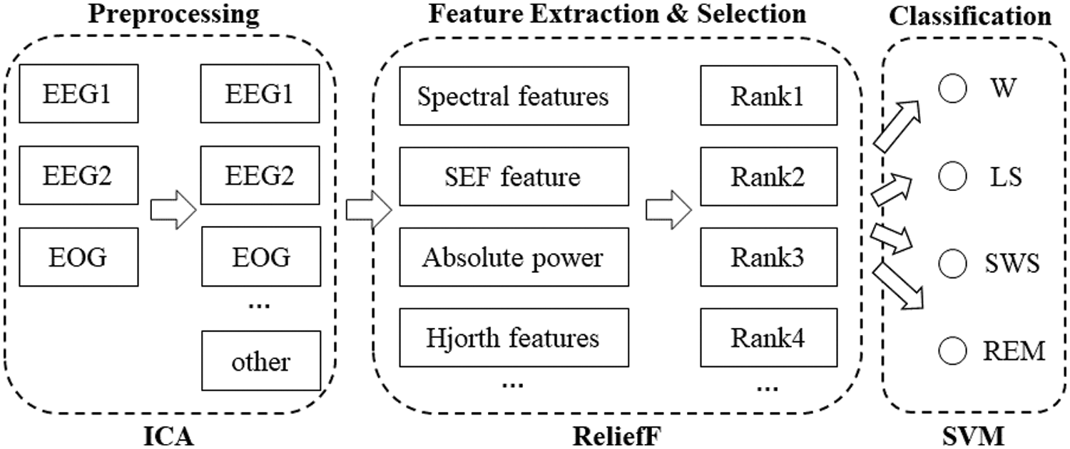
Figure 1: Flowchart of sleep stage classification using multimodal signals
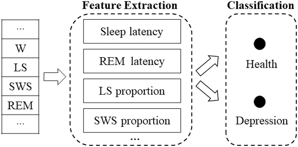
Figure 2: Depression detection algorithm
In this part, all of the EEG and EOG channels were displayed with a 0.3–35 Hz bandpass filter, and then the input sleep data were segmented into sets of 30 seconds per epoch because the sleep recordings were scored by experts according to the AASM standard. ICA, developed from blind signal separation technology, is a multichannel signal processing method. This approach is very popular among researchers who work in areas such as signal processing and speech recognition. The initial learning rate was set to
Sleep stage classification is typically performed by identifying the features extracted from cerebral rhythms, which contain time-based, frequency-based, and entropy-based features. For depression detection, the features extracted from the sleep stage labels have been used to distinguish between depressed patients and healthy people in many studies.
Spectral features: Spectral features were originally described in [23] and were first used for EEG signal analysis in [24]. Spectral features attempt to capture classification related information from the magnitude spectrum of the signal based on fast Fourier transformation. Each filtered epoch was divided into eight groups without overlapping, and we used the average value as the final spectral feature.
Spectral edge frequency features: The spectral edge frequency (SEF) is the frequency below which a certain fraction of the signal power is contained. The difference between that frequencies is generally denoted as SEFxx, where xx is the fraction of the signal power for which the edge frequency is calculated [25]. The spectral edge frequency at 50% (SEF50), shown in Eq. 1, is the frequency below which half of the signal power is present. This value is equivalent to the median frequency of the signal. SEF95 is shown in Eq. 2:
where
Absolute spectral power: In the field of sleep staging, the absolute spectral power (AP) is used to extract REM features. A repeated-measures analysis of variance showed a significant sleep stage effect for alpha band power, and alpha band power was significantly elevated in phasic REM sleep compared with that in sleep stage 4 [26]. Therefore, we set
where
Statistic features: As physiological signals, sleep EEG, EOG, EMG, respiration and temperature signals can also be analyzed by statistical analysis [27,28]. The features contain the mean, standard deviation and some parameters of the first/second derivative of the raw signals. There were 6 features for each epoch in this study.
Hjorth features: The Hjorth parameter reflects the statistical property of a signal in the time domain and includes three components: activity, mobility, and complexity [29]. The activity parameter is associated with the high-frequency components of the signal. The mobility parameter is defined as the square root of the ratio of the variance of the first derivative of the signal to that of the signal. The complexity parameter indicates how similar the shape of a signal is to that of a pure sine wave. The expressions of these parameters are as follows [30]:
where
Maximum-Minimum Distance (MMD): The MMD feature is based on the distance formula derived from the Pythagorean Theorem [1]. The idea behind this feature is to find the distance between the maximum and minimum points in each subwindow. The subwindow is set to
where
where
where
EnergySis (Esis): The basic idea of this feature is to assume that the signal has speed and energy [1]. According to (11), the speed (velocity) of the signal can be measured by using the frequency and wavelength parameters. The frequency (
where
REM latency: REM latency is the time between lying down and reaching the REM stage. Investigations have shown that REM latency is an important feature of primary depression because it is significantly longer than that for healthy controls [31–33].
Sleep latency: Sleep latency is the time from lying down to the appearance of W, and it is the sleep symptom most complained about by depressed patients [34].
LS proportion: The proportion of LS to the total sleep time is the LS proportion. The N1 and N2 periods for depressed patients are relatively short compared to those of healthy subjects [35].
SWS proportion: The proportion of SWS to the total sleep time is the SWS proportion. The shortening of SWS due to the suppression of the mechanisms responsible for regulating NREM sleep can also reflect symptoms of depression [20].
Sleep maintenance: Sleep maintenance reflects the proportion of time required to fall asleep to the amount of time spent in bed, which may play an important role in the development of depressive disorders [35,36].
Arousal times: Arousal times, the number of awakenings throughout the night, could reflect the quality of sleep, and significant increases in awakenings for depressed patients have been reported [37].
The feature selection process, which is an important part of pattern recognition and machine learning, reduces computation costs and increases classification performance. All original features are not always useful for classification or for regression tasks since, in the distribution of the dataset, some features may be irrelevant/redundant or noisy and reduce the classification performance. ReliefF is the supervised feature weighting algorithm of the filter model. This determines the extent to which feature values discriminate the instances among different classes and is used in estimating the quality of the features according to this criterion. The ReliefF algorithm has the advantage of dealing with noisy and unknown data [38,39]. For the sleep stage classification task, the ReliefF algorithm outputs a weight to indicate the corresponding relevance of each sleep feature. In this study, the Chebyshev distance measure is used instead of the Manhattan distance measure for identifying the nearest miss and nearest hit instances, which is enough to attain accurate neighborhood selection and better prediction and it completely reduces the curse of dimensionality problem. The weight of the ReliefF algorithm is calculated using the following formula:
In the small sample classification in the field of pattern recognition, K-means is a common method in unsupervised learning [40,41], while SVM is the most common method in supervised learning. SVMs, the method that has been successfully applied to classification in various domains of pattern recognition, are used for classification in this paper. The SVM is a linear discriminant that maximizes the separation between two classes based on the assumption that it improves the classifier’s generalization capability [42,43]. In this study, there are two parts using the SVM. The first part is to achieve sleep staging with Sleep-EDF and acquisition sleep data. The other part is to distinguish the subject between healthy subjects and patients with depression. The SVM classifier with the linear kernel based on the LIBSVM toolbox [44] was used to classify the data, and the remaining parameters are set to default values [45].
2.2.5 Performance Evaluation Methods
K-fold cross-validation has been widely used in automatic sleep staging [8]. The data set is first divided into k subclusters in a k-fold cross-validation test. Moreover, (k − 1) times subclusters are used in training, whereas 1 subcluster is used for testing. The process is continued until all subclusters are left outside training and tested. The success achieved in the tested data sets provides the reliability and validity degree of the employed method. The average testing success for the k-times data set is obtained to arrive at a single validity value.
Three experiments were conducted in this study, including two experiments involving automatic sleep staging with the Sleep-EDF data set and acquired sleep data and one involving depression detection. For each experiment, we used the proposed machine learning method for feature extraction and classification with an SVM. In this study, the experiments were developed in a MATLAB environment (MATLAB and Signal Processing Toolbox Release 2019b) with an Intel(R) Core(TM) i5-4210M 2.60 GHz CPU and 12 GB of installed RAM on the Windows x64 platform.
3.1 Experiment I: Sleep Staging with Sleep-EDF
This experiment was designed to evaluate the performance of our automatic sleep staging system using the public data set Sleep-EDF. Sleep data for 38 subjects from Sleep-EDF were independently applied to the system in this experiment. Data of equal proportions in each period were extracted as the training set, and the remaining data were regarded as the testing set.
As shown in Fig. 1, we first preprocessed 3 EEG and EOG channel signals with ICA and set the initial learning rate to
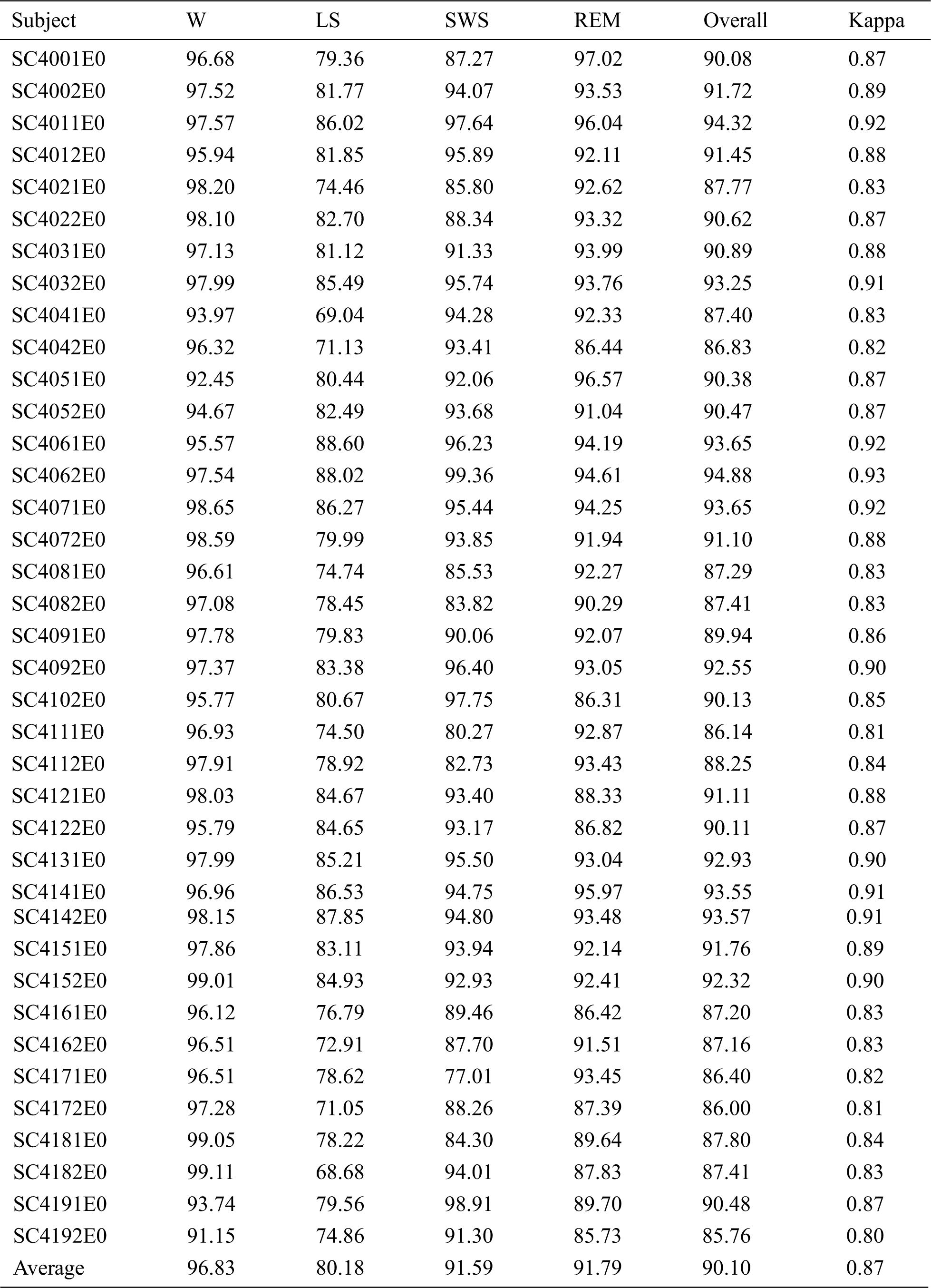
For Fpz-Cz, the average overall accuracy was 77.88 ± 6.86%, with a kappa coefficient of 0.70 ± 0.09, as shown in Tab. 1. The average accuracies of the W, LS, SWS and REM stages were 77.32%, 62.96%, 91.10% and 80.16%, respectively. The highest accuracy was 88.78%, and the lowest accuracy was 62.28%. For the multimodal signals, the overall accuracy and kappa coefficient reached 90.10 ± 2.68% and 0.87 ± 0.04, which can be seen in Tab. 2. The average accuracies of the W, LS, SWS and REM stages were 96.83%, 80.18%, 91.59% and 91.79%, respectively. The accuracies of the subjects for the W, LS and REM periods were significantly higher than those using a single channel (p < 0.01, paired t-test), especially in the W period, as shown in Fig. 3. The overall accuracy was higher than 90% for more than half of the subjects, and all the kappa coefficients were higher than 0.8. Additionally, the lowest accuracy was higher than 80%.
Table 1: Results of sleep staging with Sleep-EDF for Fpz-Cz
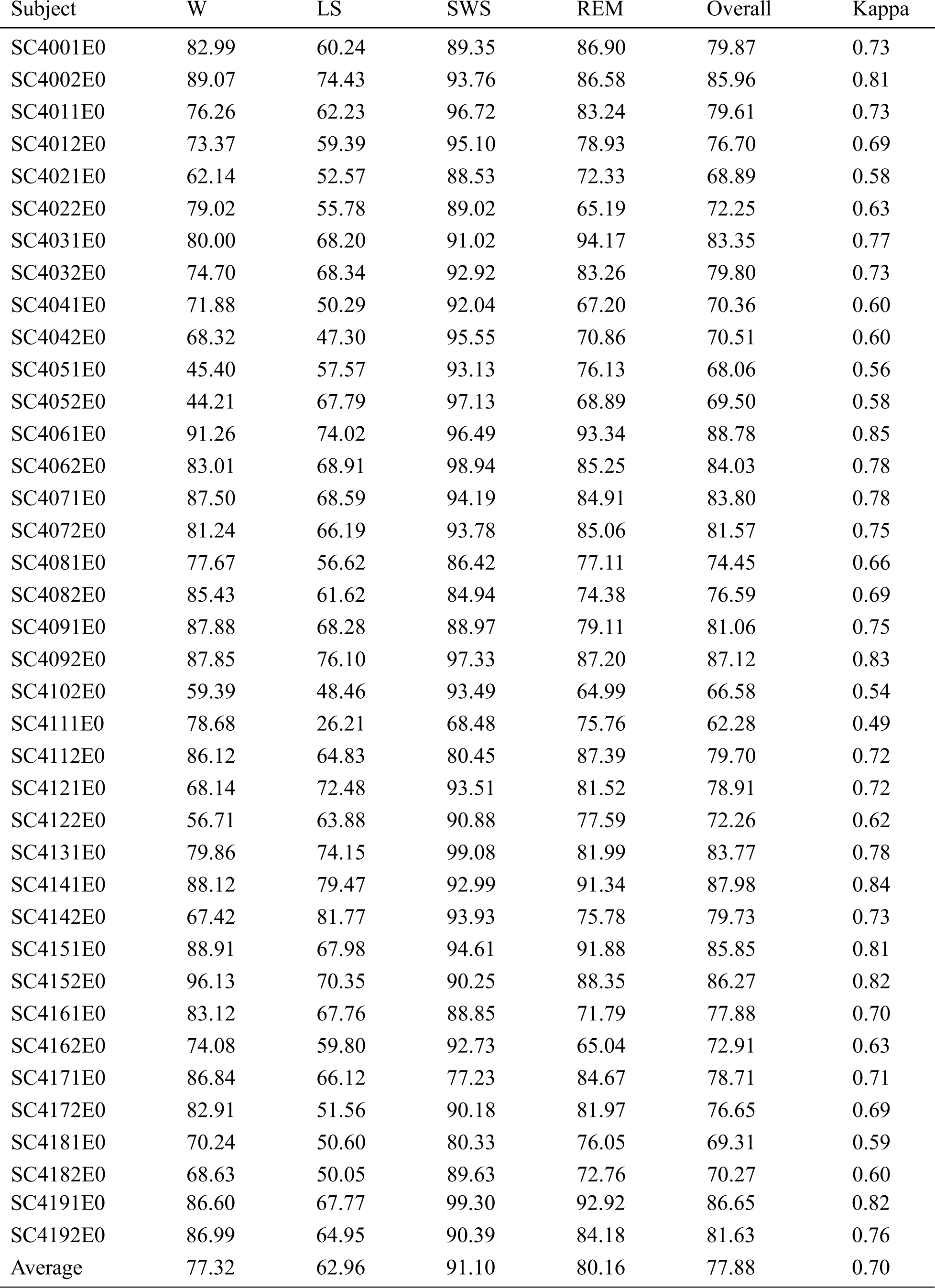
Table 2: Results of sleep staging with Sleep-EDF for multimodal signals
Although the accuracy for LS is relatively low, potentially because LS is a transitional phase between being awake and other sleep states and displays similar EEG patterns as those for REM, most sleep staging methods have similar problems. Moreover, the accuracy of W and LS is much higher than the former method. The overall accuracy for multimodal signals is 11.62% higher than that for single-channel signals, which reflects the effectiveness and reliability of the proposed method with multimodal signals and ICA preprocessing.
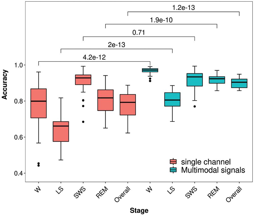
Figure 3: Box-whisker plots of Experiment I and p value with t-test
3.2 Experiment II: Sleep Staging with Raw Sleep Data
To validate the effectiveness of our method, we performed sleep staging experiments on healthy subjects and patients with depression based on the automatic sleep staging system that was optimized in Experiment I. Sleep data for 19 depressed patients and 12 healthy subjects were used in this experiment, and the data spanned an entire night. Feature vectors were extracted from the sleep data of subjects through preprocessing and feature extraction. Then, sleep staging was performed using the vectors through the SVM classifier.
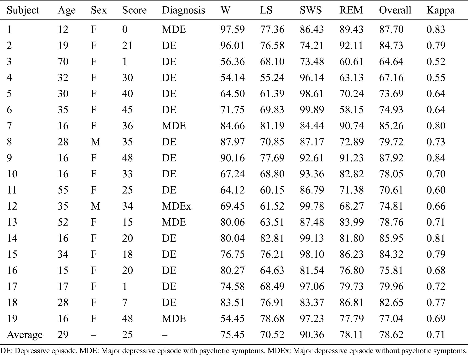
For the patients with depression, we obtained an average overall accuracy of 78.62 ± 6.71% with a kappa coefficient of 0.71 ± 0.09, as shown in Tab. 3. The accuracies of W, LS, SWS and REM were 75.45%, 70.52%, 90.36% and 78.11%, respectively. Notably, the accuracy for elderly subjects was relatively low, and that for teenagers was higher than the average value.
Table 3: Details of the depressed patients and results of the sleep staging experiments
For the healthy subjects, the overall accuracy reached 69.23 ± 5.55%, and the kappa coefficient was 0.58 ± 0.08, as shown in Tab. 4. In particular, the accuracy of W was higher than 80%, but the accuracies of LS and REM were relatively low.
Table 4: Details for healthy subjects and the results of sleep staging experiments
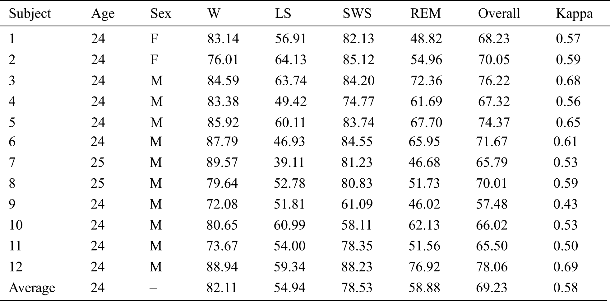
The accuracy for the LS period was relatively low for healthy subjects. In addition, the accuracy in Experiment II was lower than that in Experiment I with Sleep-EDF.
3.3 Experiment III: Depression Detection
To explore the feasibility of depression detection, we established an experiment to differentiate patients with depression and healthy subjects. The labels of patients and healthy subjects, which were manually classified by a sleep expert, were regarded as input data and added to the depression detection system. Ten labels for 4 healthy subjects and 6 depressed patients were randomly selected as the training set, and the other labels were regarded as the test set. For the label data, features were acquired, including the REM latency, sleep latency, LS proportion, SWS proportion, sleep maintenance time, arousal time, etc. Finally, the SVM classifier was used to classify patients. As reported in Tab. 5, among the test set consisting of 21 subjects (13 depressed patients and 8 healthy subjects), 20 subjects were classified correctly, so the accuracy was 95.24%. The true positive rate (TPR), false positive rate (FPR), true negative rate (TNR) and false negative rate (FNR) were 100%, 7.69%, 92.31% and 0%, respectively. Moreover, the F-score reached 94.12%, which suggests that the proposed method is effective.
Table 5: Confusion matrix for depression detection
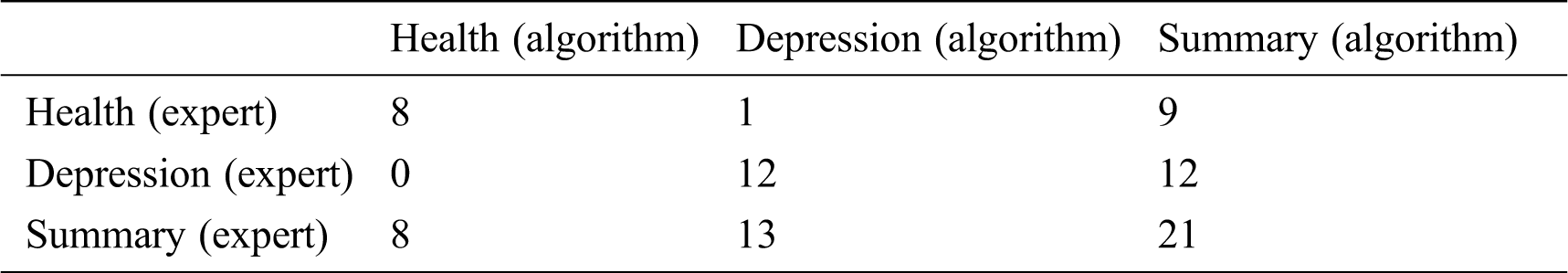
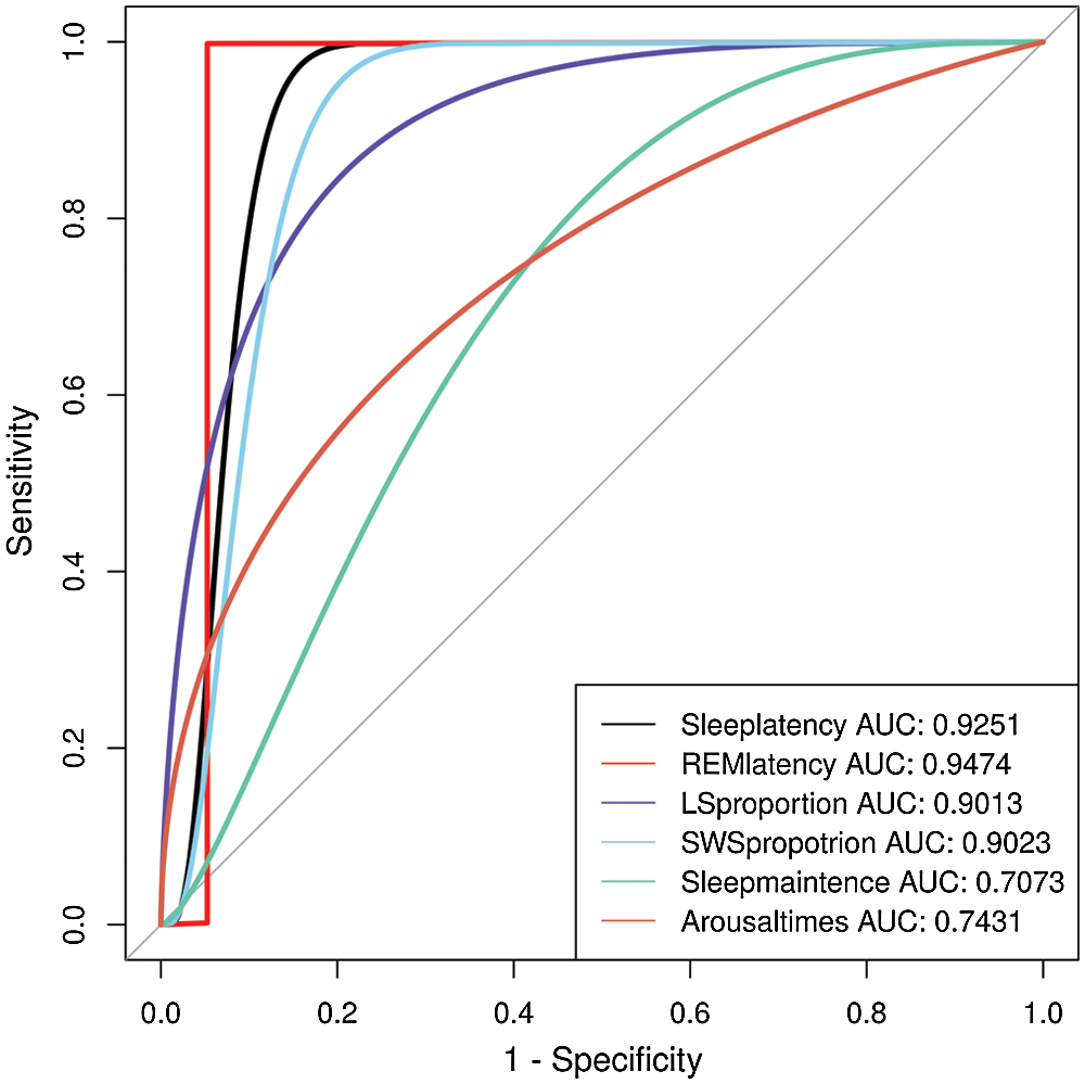
Figure 4: ROC curve of depression detection using different features
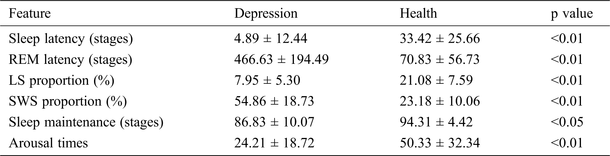
TPR and FPR are appropriate measures for evaluating the performance of depression detection. The receiver operating characteristic (ROC) curves depict the relation between the TPR and FPR. We used the extracted features to obtain the ROC curve. As shown in Fig. 4, the areas under the ROC curve are both close to 1. The conventional parameters of sleep stage labeling are summarized in Tab. 6. The depressed patient group showed several of the well-known pathognomonic sleep changes, such as decreases in the LS stage percentage, sleep latency, sleep efficiency and arousal times and increases in the REM latency and SWS stage percentage.
Table 6: Conventional sleep patterns for controls and depressed patients
This work provides a comprehensive survey of automatic multimodal signal processing techniques applied for sleep stage identification. The automatic sleep stage classification system analysis procedure was divided into four essential parts: preprocessing, feature extraction, feature selection and classification. The survey offers valuable information for researchers to determine the effectiveness of methods based on multimodal signals, and the performance and efficiency of various methods are discussed. In this study, we evaluated the proposed automatic sleep staging algorithm using the public dataset Sleep-EDF and sleep data acquired for healthy subjects and patients with depression. For Sleep-EDF, we obtained a relatively high overall accuracy using multimodal signals, reaching 90.10 ± 2.68%, and the kappa coefficient was 0.87 ± 0.04. For the sleep data obtained for patients with depression, the accuracy was 78.62 ± 6.71%, which indicates the effectiveness of the proposed system. In addition, an algorithm for depression detection was proposed. The accuracy of depression recognition was 95.24%, with an F-score of 94.12%. This finding indicates that the proposed method has certain advantages over other methods in terms of accuracy and feasibility; therefore, this research can be considered an important step toward a fully automated, convenient and efficient sleep quality evaluation system.
The proposed automatic sleep staging system took approximately 30 minutes to complete a sleep staging task for one subject. However, it takes hours for experts to perform manual sleep stage classification. Therefore, the proposed method is efficient compared to the current methods applied in practice. Although we used multimodal signals, several channels, including EEG and EOG, were used in the system. This method can be effectively applied in clinical practice. In Experiment I, the method with multimodal signals yielded an accuracy increase of greater than 10% over that for a single-channel signal (77.88 ± 6.86%). In particular for the LS period, its accuracy improved dramatically, though it has always been regarded as the most difficult period to be classified. Thus, the proposed effective multimodal signal automatic sleep staging method is highly reliable for use in automatic sleep staging systems. However, the accuracy of sleep staging of healthy subjects in Experiment 2 was not quite as good compared with that of patients. As pointed out in most clinical studies, there is a decrease of total sleep time and stage SWS and an increase of stage W in depressed patients in comparison with the healthy controls, and that increasing the difficulty of sleeping staging for the healthy subjects. Furthermore, the physiologic systems in a healthy state generate activity fluctuations on many time scales, which would also influence the accuracy of sleep staging to some extent [46].
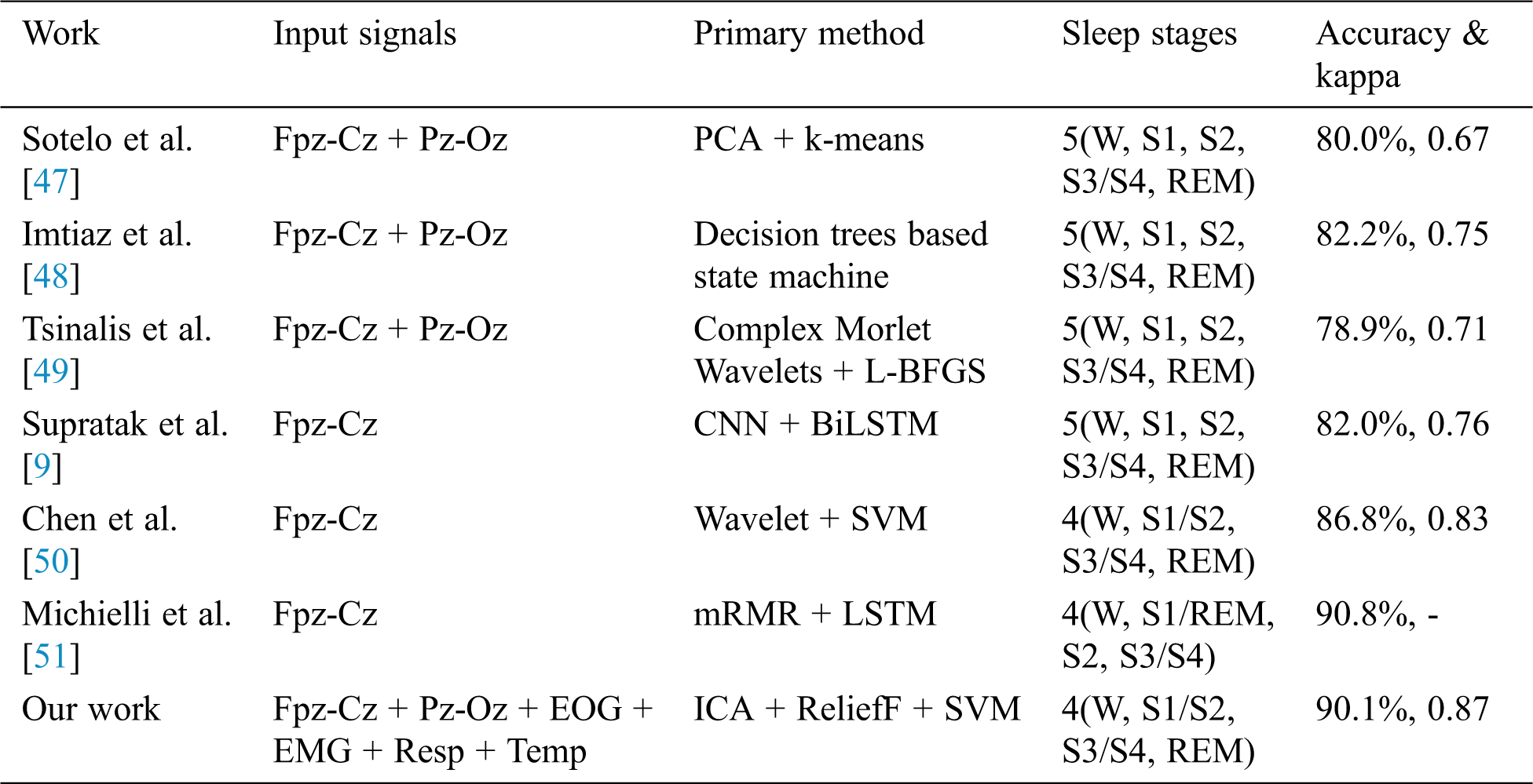
All of the methods listed in Tab. 7 utilized the Sleep-EDF dataset, and only the best accuracy is presented. As shown, the accuracy of the proposed method was 90.1%, and our proposed method achieved nearly the highest accuracy reported. There are a few factors that may contribute to the high performance of our result. First, the multimodal signals were used in this system and they could provide more information of sleep data. In other aspects, multimodal signals are suitable for ICA preprocessing to decrease noise in the signals. Second, the application of the ReliefF feature selection in sleep staging system is also an important factor. The ReliefF algorithm is used to evaluate the relevance of features to labels. Highly relevant features can commendably reflect the discrimination of samples from different classes and the similarity of samples from the same class. The trained classifier used ReliefF with the Chebyshev distance measure to capture more valid information from the new feature vector, thereby enlarging its ability to perform pattern recognition.
Table 7: Accuracy obtained in the proposed method and with previous methods based on Sleep-EDF
The accuracy variations for different patients may be because depressed patients’ sleep patterns are different from those of healthy subjects, as noted in many studies. The sleep efficiency of depressed individuals is obviously lower than that of healthy patients. Patients displayed abnormally small autocorrelations during the LS and SWS stages in comparison to healthy controls [46]. Sleep latency and REM latency are important variables that contribute to the distinction between healthy and depressed people [15,52]. Additionally, there is enough evidence provided by other parameters, such as sleep maintenance and REM activity, to indicate the differences between healthy and depressed individuals [53]. In other words, physiological systems in a healthy state generate activity fluctuations on many time scales, and disease states are associated with a breakdown of this traditional temporal structure. Although the numbers of healthy and depressed subjects studied were relatively small, an accuracy rate of up to 95.24% was achieved, indicating that the proposed method provides a viable way to automatically recognize depression with computers.
The limitations of this study are primarily related to data acquisition and the proposed methodology. The raw sleep data collected, especially for healthy subjects, may have too much noise to yield high-accuracy results in sleep staging analyses. In addition, the sleep stage labels used for depression detection were not manually divided by experts because the accuracy of the results of Experiment II was not high enough to support depression recognition.
Future work will consider artificial neural networks to enable us to efficiently improve the performance of automatic sleep staging [54]. Additionally, we will further explore the difference between the sleep patterns of patients with depression and healthy people and attempt to automatically detect them.
Conflicts of Interest: The authors declare that there are no conflicts of interest regarding the publication of this paper.
Funding Statement: This study was supported by the Key Realm R and D Program of Guangzhou under grant 202007030005, the National Natural Science Foundation of China under grants 62076103 and 61906019, the Guangdong Natural Science Foundation under grant 2019A1515011375, and the Natural Science Foundation of Hunan Province under grant 2019JJ50649.
1. K. A. I. Aboalayon, M. Faezipour, W. S. Almuhammadi and S. Moslehpour. (2016). “Sleep stage classification using EEG signal analysis: a comprehensive survey and new investigation,” Entropy, vol. 18, no. 9, pp. 272. [Google Scholar]
2. A. Rechtschaffen and A. Kales. (1968). “A manual of standardized terminology, techniques and scoring system of sleep stages in human subjects,” Los Angeles, CA, USA: Brain Information Service, pp. 1–58. [Google Scholar]
3. R. B. Berry, R. Brooks, C. E. Gamaldo, S. M. Harding, C. Marcus et al. (2012). , “The AASM manual for the scoring of sleep and associated events,” American Academy of Sleep Medicine, vol. 176, pp. 2012. [Google Scholar]
4. Z. He, Z. Li, F. Yang, L. Wang, J. Li et al. (2020). , “Advances in multimodal emotion recognition based on Brain-Computer Interfaces,” Brain Sciences, vol. 10, no. 10, pp. 687. [Google Scholar]
5. H. Jiang, Z. Wang, R. Jiao and S. Jiang. (2020). “Picture-induced EEG signal classification based on CVC emotion recognition system,” Computers, Materials & Continua, vol. 65, no. 2, pp. 1453–1465. [Google Scholar]
6. Y. Tan, L. Tan, X. Xiang, H. Tang, J. Qin et al. (2020). , “Automatic detection of aortic dissection based on morphology and deep learning,” Computers, Materials & Continua, vol. 62, no. 3, pp. 1201–1215. [Google Scholar]
7. Z. L. Yang, S. Y. Zhang, Y. T. Hu, Z. W. Hu and Y. F. Huang. (2020). “VAE-Stega: linguistic steganography based on variational auto-encoder,” IEEE Transactions on Information Forensics Security, vol. 16, pp. 880–895. [Google Scholar]
8. B. Şen, M. Peker, A. Çavuşoğlu and F. V. Çelebi. (2014). “A comparative study on classification of sleep stage based on EEG signals using feature selection and classification algorithms,” Journal of Medical Systems, vol. 38, no. 3, pp. 18. [Google Scholar]
9. A. Supratak, H. Dong, C. Wu and Y. Guo. (2017). “DeepSleepNet: a model for automatic sleep stage scoring based on raw single-channel EEG,” IEEE Transactions on Neural Systems and Rehabilitation Engineering, vol. 25, no. 11, pp. 1998–2008. [Google Scholar]
10. S. Mousavi, F. Afghah and U. R. Acharya. (2019). “SleepEEGNet: automated sleep stage scoring with sequence to sequence deep learning approach,” PloS One, vol. 14, no. 5, pp. e0216456. [Google Scholar]
11. H. Ghimatgar, K. Kazemi, M. S. Helfroush and A. Aarabi. (2019). “An automatic single-channel EEG-based sleep stage scoring method based on hidden Markov Model,” Journal of Neuroscience Methods, vol. 324, pp. 108320. [Google Scholar]
12. M. M. Rahman and M. I. H. Bhuiyan. (2019). “Sleep stage classification using EOG signals with reduced class imbalance effect,” in 2019 IEEE Int. Conf. on Biomedical Engineering, Computer and Information Technology for Health (BECITHCONDhaka, Bangladesh, pp. 81–84. [Google Scholar]
13. H. Phan, F. Andreotti, N. Cooray, O. Y. Chén and M. De Vos. (2019). “Joint classification and prediction CNN framework for automatic sleep stage classification,” IEEE Transactions on Biomedical Engineering, vol. 66, no. 5, pp. 1285–1296. [Google Scholar]
14. S. Kang and T. Park. (2019). “Detecting outlier behavior of game player players using multimodal physiology data,” Intelligent Automation & Soft Computing, vol. 2019, pp. 1–10. [Google Scholar]
15. J. C. Gillin, W. Duncan, K. D. Pettigrew, B. L. Frankel and F. Snyder. (1979). “Successful separation of depressed, normal, and insomniac subjects by EEG sleep data,” Archives of General Psychiatry, vol. 36, no. 1, pp. 85–90. [Google Scholar]
16. N. Tsuno, A. Besset and K. Ritchie. (2005). “Sleep and depression,” Journal of Clinical Psychiatry, vol. 66, no. 10, pp. 1254–1269. [Google Scholar]
17. N. Schaltenbrand, R. Lengelle, M. Toussaint, R. Luthringer, G. Carelli et al. (1996). , “Sleep stage scoring using the neural network model: comparison between visual and automatic analysis in normal subjects and patients,” Sleep, vol. 19, no. 1, pp. 26–35. [Google Scholar]
18. M. Hamilton. (1967). “Development of a rating scale for primary depressive illness,” British Journal of Social and Clinical Psychology, vol. 6, no. 4, pp. 278–296. [Google Scholar]
19. H. Cai, J. Han, Y. Chen, X. Sha, Z.Wang et al. (2018). , “A pervasive approach to EEG-based depression detection,” Complexity, vol. 2018, pp. 5238028. [Google Scholar]
20. V. Pillai, D. A. Kalmbach and J. A. Ciesla. (2011). “A meta-analysis of electroencephalographic sleep in depression: evidence for genetic biomarkers,” Biological Psychiatry, vol. 70, no. 10, pp. 912–919. [Google Scholar]
21. B. Kemp, A. H. Zwinderman, B. Tuk, H. A. Kamphuisen and J. J. Oberye. (2000). “Analysis of a sleep-dependent neuronal feedback loop: the slow-wave microcontinuity of the EEG,” IEEE Transactions on Biomedical Engineering, vol. 47, no. 9, pp. 1185–1194. [Google Scholar]
22. S. Makeig, A. J. Bell, T. P. Jung and T. J. Sejnowski. (1996). “Independent component analysis of electroencephalographic data,” in Advances in Neural Information Processing Systems. Denver, CO, USA, 145–151. [Google Scholar]
23. G. Peeters. (2004). “A large set of audio features for sound description (similarity and classification) in the CUIDADO project,” CUIDADO IST Project Report, vol. 54, no. 0, pp. 1–25. [Google Scholar]
24. A.-C. Conneau and S. Essid. (2014). “Assessment of new spectral features for eeg-based emotion recognition,” in 2014 IEEE Int. Conf. on Acoustics, Speech and Signal Processing (ICASSPFlorence, Italy, pp. 4698–4702. [Google Scholar]
25. S. A. Imtiaz and E. Rodriguez-Villegas. (2014). “A low computational cost algorithm for REM sleep detection using single channel EEG,” Annals of Biomedical Engineering, vol. 42, no. 11, pp. 2344–2359. [Google Scholar]
26. U. Ermis, K. Krakow and U. Voss. (2010). “Arousal thresholds during human tonic and phasic REM sleep,” Journal of Sleep Research, vol. 19, no. 3, pp. 400–406. [Google Scholar]
27. P. C. Petrantonakis and L. J. Hadjileontiadis. (2009). “Emotion recognition from EEG using higher order crossings,” IEEE Transactions on information Technology in Biomedicine, vol. 14, no. 2, pp. 186–197. [Google Scholar]
28. K. Takahashi. (2004). “Remarks on emotion recognition from bio-potential signals,” in 2nd Int. Conf. on Autonomous Robots and Agents, Palmerston North, New Zealand, pp. 186–191. [Google Scholar]
29. S. H. Oh, Y. R. Lee and H. N. Kim. (2014). “A novel EEG feature extraction method using Hjorth parameter,” International Journal of Electronics and Electrical Engineering, vol. 2, no. 2, pp. 106–110. [Google Scholar]
30. P. Memar and F. Faradji. (2018). “A novel multi-class EEG-based sleep stage classification system,” IEEE Transactions on Neural Systems Rehabilitation Engineering, vol. 26, no. 1, pp. 84–95. [Google Scholar]
31. D. Kupfer. (1976). “REM latency: a psychobiologic marker for primary depressive disease,” Biological Psychiatry, vol. 11, no. 2, pp. 159. [Google Scholar]
32. J. C. Gillin, T. L. Smith, M. Irwin, D. F. Kripke, S. Brown et al. (1990). , “Short REM latency in primary alcoholic patients with secondary depression,” American Journal of Psychiatry, vol. 147, no. 1, pp. 9. [Google Scholar]
33. D. J. Kupfer, F. G. Foster, L. Reich, K. S. Thompson and B. Weiss. (1976). “EEG sleep changes as predictors in depression,” American Journal of Psychiatry, vol. 133, no. 6, pp. 622. [Google Scholar]
34. P. A. Vanable, J. E. Aikens, L. Tadimeti, B. Caruana-Montaldo and W. B. Mendelson. (2000). “Sleep latency and duration estimates among sleep disorder patients: variability as a function of sleep disorder diagnosis, sleep history, and psychological characteristics,” Sleep: Journal of Sleep Research & Sleep Medicine, vol. 23, no. 1, pp. 71–79. [Google Scholar]
35. C. F. Reynolds III, D. J. Kupfer, L. S. Taska, C. C. Hoch, D. G. Spiker et al. (1985). , “EEG sleep in elderly depressed, demented, and healthy subjects,” Biological Psychiatry, vol. 20, no. 4, pp. 431–442. [Google Scholar]
36. E. M. Park, S. Meltzer-Brody and R. Stickgold. (2013). “Poor sleep maintenance and subjective sleep quality are associated with postpartum maternal depression symptom severity,” Archives of Women’s Mental Health, vol. 16, no. 6, pp. 539–547. [Google Scholar]
37. J. Staedt, H. Hünerjäger, E. Rüther and G. Stoppe. (1998). “Sleep cluster arousal analysis and treatment response to heterocyclic antidepressants in patients with major depression,” Journal of Affective Disorders, vol. 49, no. 3, pp. 221–227. [Google Scholar]
38. I. Kononenko. (1994). “Estimating attributes: analysis and extensions of RELIEF,” in European Conf. on Machine Learning, Berlin, Heidelberg, pp. 171–182. [Google Scholar]
39. B. Chen, G. Zhu, M. Ji, Y. T. Yu, J. Zhao et al. (2020). , “Air quality prediction based on Kohonen clustering and ReliefF feature selection,” Computers, Materials & Continua, vol. 64, no. 2, pp. 1039–1049. [Google Scholar]
40. A. A. M. Jamel and B. Akay. (2019). “A survey and systematic categorization of parallel K-means and Fuzzy-c-means algorithms,” Computer Systems Science and Engineering, vol. 34, no. 5, pp. 259–281. [Google Scholar]
41. P. Tang, Y. Wang and N. Shen. (2020). “Prediction of college students’ physical fitness based on K-means clustering and SVR,” Computer Systems Science and Engineering, vol. 35, no. 4, pp. 237–246. [Google Scholar]
42. J. Pan, Y. Li and J. Wang. (2016). “An EEG-based brain-computer interface for emotion recognition,” in 2016 Int. Joint Conf. on Neural Networks (IJCNNVancouver, BC, Canada, pp. 2063–2067. [Google Scholar]
43. Xiang L., Yang S., Liu Y., Li Q. and Zhu C. (2020). “Novel linguistic steganography based on character-level text generation,” Mathematics, vol. 8, no. 9, pp. 1558. [Google Scholar]
44. C.-C. Chang and C.-J. Lin. (2011). “LIBSVM: a library for support vector machines,” ACM Transactions on Intelligent Systems and Technology, vol. 2, no. 3, pp. 1–27. [Google Scholar]
45. Z. Li, L. Qiu, R. Li, Z. He, J. Xiao et al. (2020). , “Enhancing BCI-based emotion recognition using an improved Particle Swarm Optimization for feature selection,” Sensors, vol. 20, no. 11, pp. 3028. [Google Scholar]
46. S. Leistedt, M. Dumont, J. P. Lanquart, F. Jurysta and P. Linkowski. (2007). “Characterization of the sleep EEG in acutely depressed men using detrended fluctuation analysis,” Clinical Neurophysiology, vol. 118, no. 4, pp. 940–950. [Google Scholar]
47. J. Rodríguez-Sotelo, A. Osorio-Forero, A. Jiménez-Rodríguez, D. Cuesta-Frau, E. Cirugeda-Roldán et al. (2014). , “Automatic sleep stages classification using EEG entropy features and unsupervised pattern analysis techniques,” Entropy, vol. 16, no. 12, pp. 6573–6589. [Google Scholar]
48. S. A. Imtiaz and E. Rodriguez-Villegas. (2015). “Automatic sleep staging using state machine-controlled decision trees,” in 2015 37th Annual Int. Conf. of the IEEE Engineering in Medicine and Biology Society (EMBCMilan, Italy, pp. 378–381. [Google Scholar]
49. O. Tsinalis, P. M. Matthews and Y. Guo. (2016). “Automatic sleep stage scoring using time-frequency analysis and stacked sparse autoencoders,” Annals of Biomedical Engineering, vol. 44, no. 5, pp. 1587–1597. [Google Scholar]
50. T. Chen, H. Huang, J. Pan and Y. Li. (2018). “An EEG-based brain-computer interface for automatic sleep stage classification,” in 2018 13th IEEE Conf. on Industrial Electronics and Applications (ICIEAWuhan, Hubei, China, pp. 1988–1991. [Google Scholar]
51. N. Michielli, U. R. Acharya and F. Molinari. (2019). “Cascaded LSTM recurrent neural network for automated sleep stage classification using single-channel EEG signals,” Computers in Biology and Medicine, vol. 106, pp. 71–81. [Google Scholar]
52. P. Coble, F. G. Foster and D. J. Kupfer. (1976). “Electroencephalographic sleep diagnosis of primary depression,” Archives of General Psychiatry, vol. 33, no. 9, pp. 1124–1127. [Google Scholar]
53. D. J. Kupfer, R. F. Ulrich, P. A. Coble, D. B. Jarrett, V. Grochocinski et al. (1984). , “Application of automated REM and slow wave sleep analysis: I. Normal and depressed subjects,” Psychiatry Research, vol. 13, no. 4, pp. 325–334. [Google Scholar]
54. J. Zhu, Z. Wang, T. Gong, S. Zeng, X. Li et al. (2020). , “An improved classification model for depression detection using EEG and eye tracking data,” IEEE Transactions on NanoBioscience, vol. 19, no. 3, pp. 527–537. [Google Scholar]
 | This work is licensed under a Creative Commons Attribution 4.0 International License, which permits unrestricted use, distribution, and reproduction in any medium, provided the original work is properly cited. |