DOI:10.32604/iasc.2021.016246
| Intelligent Automation & Soft Computing DOI:10.32604/iasc.2021.016246 | |
| Article |
Hybrid Deep Learning Modeling for Water Level Prediction in Yangtze River
1School of Energy and Power Engineering, Wuhan University of Technology, Wuhan, 430070, China
2School of Automation, Wuhan University of Technology, Wuhan, 430070, China
3University of New South Wales, Sydney, NSW, 2052, Australia
*Corresponding Author: Zhaoqing Xie. Email: youzicha2012@163.com
Received: 28 December 2020; Accepted: 06 February 2021
Abstract: Accurate prediction of water level in inland waterway has been an important issue for helping flood control and vessel navigation in a proactive manner. In this research, a deep learning approach called long short-term memory network combined with discrete wavelet transform (WA-LSTM) is proposed for daily water level prediction. The wavelet transform is applied to decompose time series into details and approximation components for a better understanding of temporal properties, and a novel LSTM network is used to learn generic water level features through layer-by-layer feature granulation with a greedy layer wise unsupervised learning algorithm. Six representative reaches in Yangtze River, namely, the Jianli, Wuhan, Jiujiang, Anqing, Wuhu, and Nanjing are investigated, and water level data from 2010 to 2019 are processed through temporal and spatial correlation analysis, and combination-optimized to develop and evaluate the proposed model. In general, the test average performances on RMSE and MAE are less than 0.045 m and 0.035 m respectively, which outperforms the state-of-the-art models, such as WA-ANN, WA-ARIMA and LSTM models. The results indicate that the WA-LSTM model is stable, reliable and widely applicable.
Keywords: LSTM; wavelet; water level prediction; Yangtze River
The Yangtze River, being the longest river in China and the third longest river in the world, runs across China from west to east, plays a vital role in the economic development. Water level prediction is not only helpful for flood control in flood season and vessel navigation in dry season, but also conducive for waterway regulation, port management, etc. Thus, accurately and timely prediction is particularly necessary.
In recent decades, a wide variety of approaches have been investigated for water level prediction, mainly divided into model-driven and data-driven methods. The model-driven methods include experience formulas between water level and water flow [1], generalized extreme value distributions [2], Muskingum model parameters optimal estimation [3], mathematical expression between water level and tide [4], etc. Generally, these models are parameter-based, frequently make a number of hypotheses ideal circumstances, depend on hand-crafted features that are expensive to create and require expert knowledge of the field, in addition, they mainly focus on univariate data excluding the complex joint distributions, resulting in sensitive to disturb. However, water level system in Yangtze River is complicated and uncertain, from the long-term variation trends. Zhang [5] analyzed the annual maximum water level and stream flow during the 1877–2000 year in the Yangtze river basin, and concluded that the periods of water level changes were decreasing over time. Liu [6] explored the annual proportion of flood and dry seasons, and suggested that the water level will emerge an irregular change. As for the factors influencing water level as concerned, such as rainfall-runoff [7], tidal [4], three gorges reservoir [8], natural and anthropogenic changes [9] can dramatically affect the performance of prediction. Thus, the use of model-driven models would be disadvantageous in operational use.
The data-driven models, in the early periods, representative of shallow neural networks, including support vector regression [10,11], artificial neural network [12–16] and hybrid models [17], these models are non-parameter-based, which have the ability to approximate the distribution probability of water level system regardless of its degree of non-linearity and prior knowledge, and have been demonstrated to be effective solutions for hydrological prediction. Based on these models, some algorithms are investigated to improve prediction capabilities, such as Levenberg-Marquard [18], feed-forward back-propagation [19], generalized regression and radial basis function [20], differential evolution, artificial bee colony and ant colony optimization [21], etc.
Neural networks can be specified an arbitrary number of input features, providing support for multivariate prediction, many studies have concentrated on input features selection and extraction, such as stochastic continuum temporal combinations of water level in previous time steps [22], the objective basis on which historical water level have temporal impact on the future. Spatial combinations of different locations according to the travel time that water flows to the downstream [23], the incentive origin is that water level in different locations are spatially dependent, knowledge sharing is practical. Wavelet transform to decompose time series into wavelet components [24–27], which is useful to obtain the periodic components of the measured data, stationarity transform by difference operation that could help explore any other systematic signals for better prediction.
Despite the huge improvements in water level prediction achieved by the above methods, the shallow neural networks that do not have memory, which fail to capture the long-term evolution and can only learn a mapping between input and output patterns, thus incapability to extract the overall temporal interaction of multiple inputs. Recently, deep neural networks called deep learning, has dramatically brought about breakthroughs to the shallow neural networks [28,29], including deep belief network (DBN), convolutional neural network (CNN), stack auto-encoder (SAE) and recurrent neural network (RNN), etc., these models are composed of multiple processing layers to learn representation of features with multiple levels of abstraction, have get great achievements in processing images, video, speech and text, etc. Unlike use the echo state in RNN as a supplier of interesting dynamics from which the desired output is combined, the long short-term memory network (LSTM) [30], a typical RNN, use memory block to store information for an arbitrary duration, effective at capturing long-term temporal correlations in a sequence without suffering from the optimization hurdles that plague simple recurrent networks, which may greatly improve prediction accuracy [31].
In this paper, we propose a deep-learning-based prediction model. Herein, a novel LSTM network is used to learn generic water level features through layer-by-layer feature granulation with a greedy layer wise unsupervised learning algorithm, and the discrete wavelet transform is applied to help to extract the features preliminarily for performance improvement. The remainder of this paper is organized as follows. Section 2 introduces the prediction methodology. Section 3 introduces the study area. Section 4 proposes the prediction model. Section 5 shows the experimental results and some discussions. The conclusions are drawn in Section 6.
LSTM is a special kind of RNN, unlike the repeating module in hidden layer has a very simple structure, such as a single tanh layer in standard RNN, it is known as memory blocks in LSTM, each memory block contains one or more self-connected memory cells and three multiplicative units: input gate, output gate and forget gate. The input gate can allow incoming signal to alter the state of the memory cell or block it, the output gate allows the state of the memory cell to have an effect on other neurons or prevent it, the forget gate decides when to forget the output results and thus selects the optimal time lag for the input sequence, this special structure has the ability of bridging very long time lags.
The discrete wavelet transform (DWT) has recently become a very popular when it comes to analysis and denoising time series [32,33], which is used to decompose time series into a series of wavelet components including both spectral and temporal information, and is beneficial to the detailed analysis in contrast to the Fourier transform that only elucidates frequency information. The corresponding family of the base wavelet is expressed as:
where
The coefficients
The reference decomposition level
where
In this study, the discrete wavelet transform is combined with the LSTM network for water level prediction in one day ahead, the combination model WA-LSTM is shown in Fig. 1, mainly includes four processes in the following order:
1. The feature selection to determine
2. The feature decomposition using wavelet function to transform each input feature
3. The decomposed feature learning and prediction using LSTM network separately, the predicted values are
4. The feature reconstruction using wavelet function to get the predicted water level
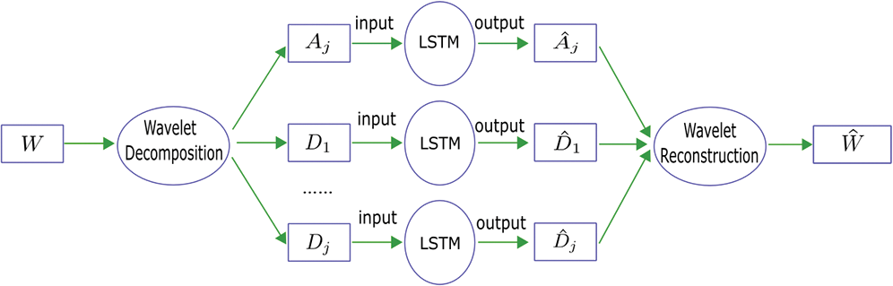
Figure 1: The prediction structure of the WA-LSTM model
In shallow neural networks, the most widely used training algorithm is error back-propagation, while it has been proven too difficult to train deep neural networks, empirically no better and often worse, a reasonable explanation is that gradient-based optimization starting from random initialization may get stuck near poor solutions. Recently, Hinton [28] has developed a greedy layer-wise unsupervised learning algorithm that can train deep networks successfully. The training strategy mainly includes three aspects, which can be stated as follows:
1. Design the architecture of the networks, and initialize parameters including weight matrices and bias vectors randomly.
2. Pre-training the first layer at a time in a greedy way, using unsupervised learning from bottom layer to top layer in order to preserve feature information from the input;
3. Fine-tuning the whole network by using back propagation method with gradient-based optimization from top layer to bottom layer in a supervised way, for searching optimal parameters by minimizing the cost function defined as:
where
In this study, six routine surveillance reaches in the middle and lower of Yangtze River, including Jianli, Wuhan, Jiujiang, Anqing, Wuhu and Nanjing are considered as the case study areas (Fig. 2). Water level is measured daily according to the ‘Wusong zero’ baseline, datasets are obtained from the Changjiang Maritime Safety Administration, and collected from January 1, 2010 to December 12, 2019.
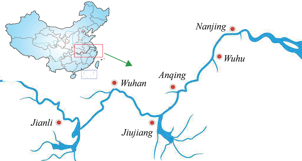
Figure 2: Study reaches in the middle and lower of Yangtze River
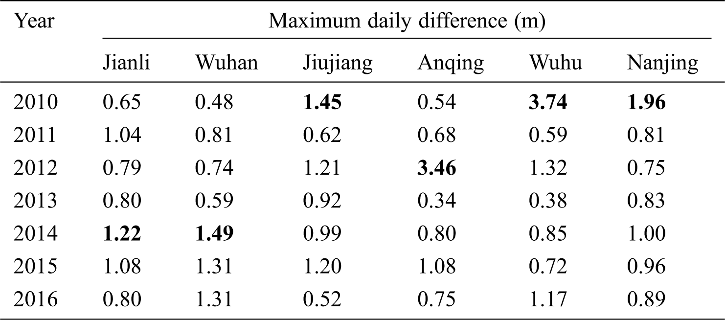
Water level in Yangtze River changes daily and shows periodically trends. For instance, the Jianli reaches, in Fig. 3, during 2010–2016, water level experienced three well defined periods: months of 1, 2, 3, 12 were in dry water period; months of 4, 5, 10, 11 were in moderate water period; months of 6, 7, 8, 9 were in flood period. In addition, it would seem obviously that water levels were different and highly irregular at the same time in the past, also, from Tab. 1, it shows clearly that the maximum daily water level difference of different year were quite different, which will bring great challenges to accurate prediction.
Table 1: The maximum daily water level differences in 2010–2016 at each reaches
Water level differ from the upstream to the downstream. Fig. 4 shows the changes of the proposed reaches in 2010, it appeared that water level presented synchronous trends at Jianli, Wuhan, Jiujiang and Anqing reaches over time, and gradually descended from the upstream to the downstream except Jianli reaches, the same phenomenon can be also found in Wuhu and Nanjing reaches.
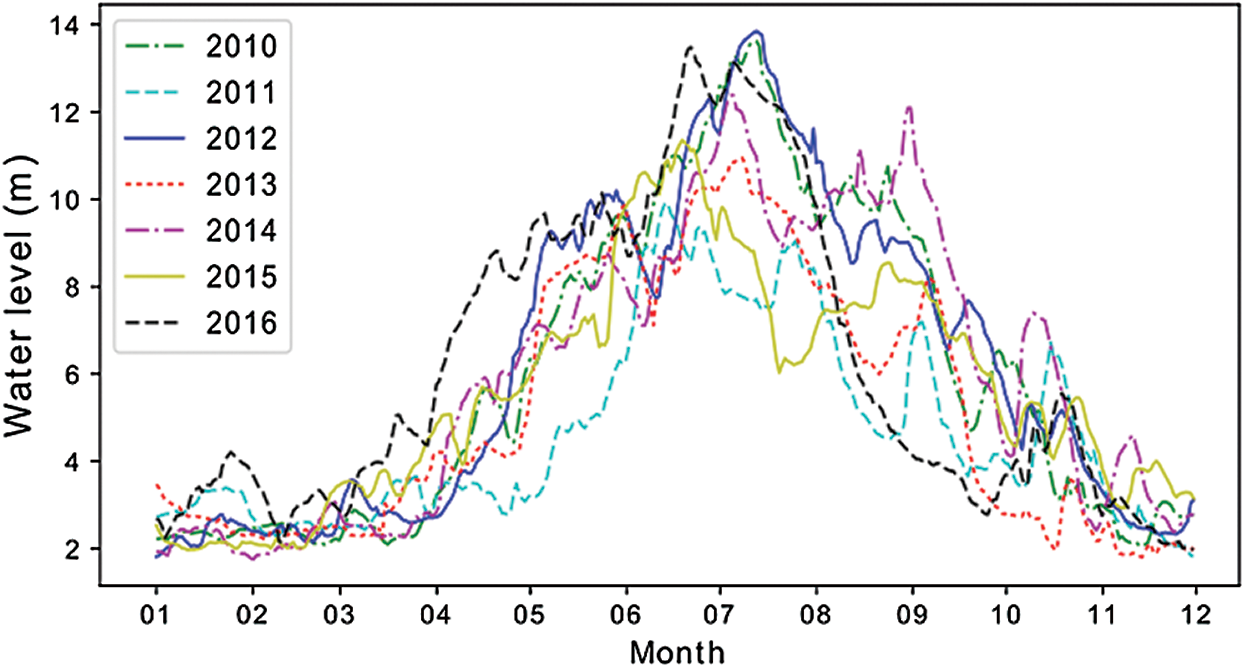
Figure 3: Water level trends of years in Jianli reaches

Figure 4: Water level trends of reaches in 2010
4 WA-LSTM Model for Water Level Prediction
In neural network models, one of the most important issues for model training is to determine the input features, in order to provide the best available input pattern for LSTM network, the correlation coefficients are calculated based on the coefficient of determination
where
Table 2: The temporal correlation coefficients between observed water level
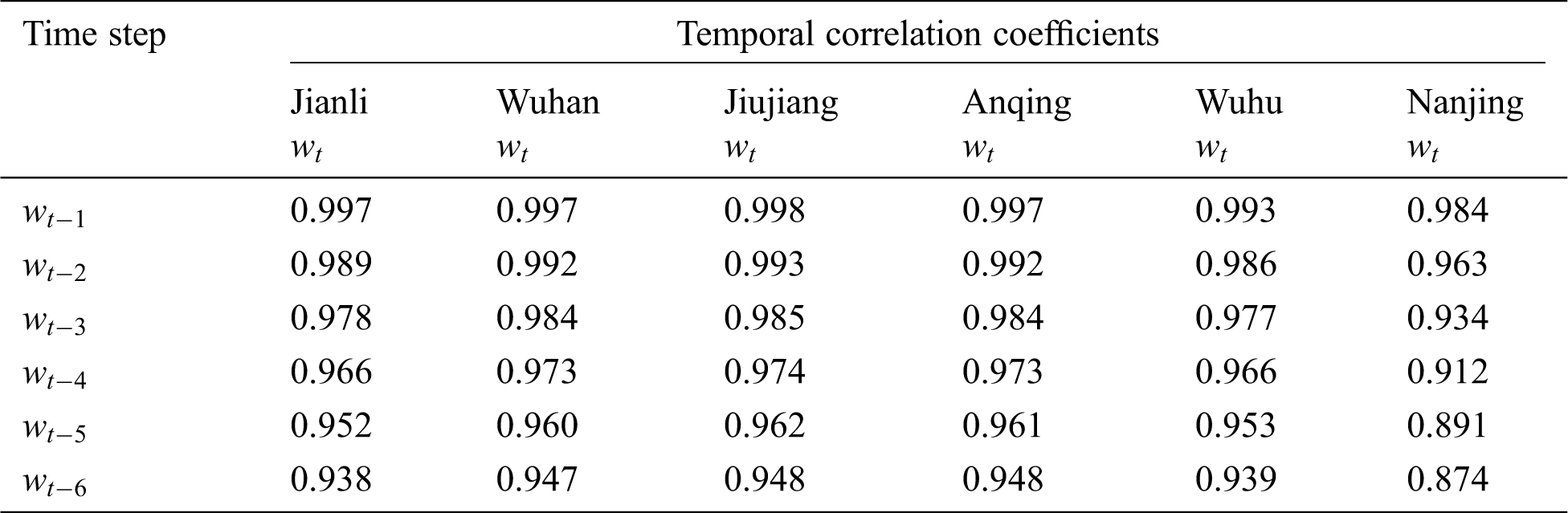
Table 3: The spatial correlation coefficients of observed water level

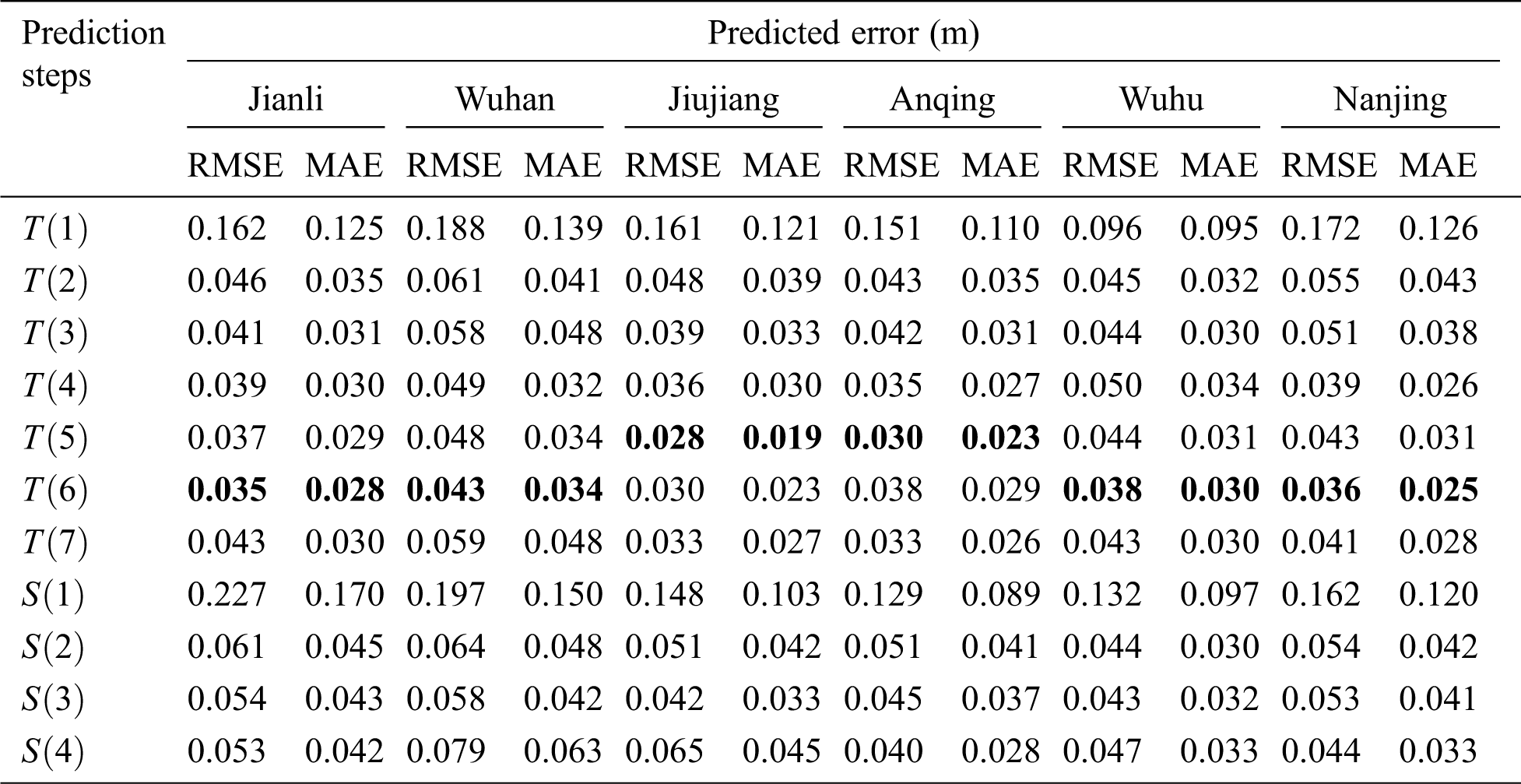
Considering the correlation analysis in Tabs. 2 and 3, the following prediction functions are defined in Tab. 4, in which, the temporal correlation is investigated to explore the temporal dependence of each reaches depend on the multi-step lag observations of historical data, while the spatial-temporal correlation extends to research the spatial and temporal correlation between different reaches.
Table 4: The Prediction functions studied in this paper

4.2 Input Features Wavelet Transform
LSTM network is sensitive to the scale of input data, specifically when the tanh and relu activation functions are used. In addition, from Fig. 3, we can see that water level show large scale irregular variations and local abrupt changes, which are not propitious for prediction and necessary to be preprocessed. In the WA-LSTM model, the discrete wavelet transform is employed to discompose water level into a series of local features, which is useful for detecting transient or singular points, and would help to overcome the difficulties.
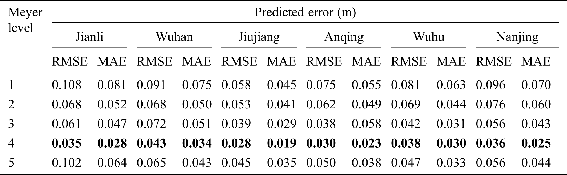
The discrete wavelet transform process mainly contains two aspects, one is to select an appropriate wavelet function as mother wavelet, the widely used are haar, db2, meyer, sym1, bior1.1, rboi1.1 and coif1 wavelets. The other critical point is to determine the decomposition level, according to the Eq. (5), the reference decomposition level is approximately 3 (N = 2556). In this study, not only the sensitivity of the wavelet type but also the decomposition level are investigated to make a comprehensive comparative study, in that case, the selected input features will be decomposed to 1, 2, 3, 4, and 5 levels by the seven different kinds of wavelet transforms.
In order to evaluate the performances of the proposed model for water level prediction, two widely used criteria are applied to measure the error of the predicted data, they are the Root Mean Squared Error (RMSE), Mean Absolute Error (MAE). The mathematical equations are defined as:
where
In order to train the WA-LSTM model parameters and prove its predictive ability, the dataset is split into two parts, the first 70% dataset is used as the training sample, while the remaining 30% is employed as testing sample for measuring prediction performance of the proposed networks.
5.1 Optimum Parameters Analysis
The effectiveness of deep learning highly depends on the LSTM network topology, before applying WA-LSTM to the dataset, some appropriate hyper-parameters must be fitted. As shown in Tab. 5, the value of hidden layer determines the depth of the LSTM, the hidden layer neurons reflect the width, the batch size is an optimization in the training of the network, defining how many patterns to read at a time and keep in memory, and the epochs represents the number of times the network is optimally trained. Since the WA-LSTM model has many parameters needed to be set, parameter optimization is notoriously difficult to implement. In this paper, an effective method is worked out by grid search technology to address the issue. By experiments, we find that the most suitable wavelet transform is the Meyer wavelet with decomposition level 4, and for all the decomposed components, the optimum parameters of WA-LSTM are shown in Tab. 5, which suggests that different frequency component should use different model parameters.
Table 5: Optimum model parameters of WA-LSTM model

5.2 Temporal and Spatial Correlation Analysis
According to Tab. 6, the best prediction steps for different reaches are similar, which means 5 or 6 days lag observations as an input features best predict daily water level. The temporal dependence is much longer when compared with other approaches usually with only 2 or 3 [34], this can be explained from two aspects: one is that the temporal correlation keeps at a comparatively high level according to Tab. 2, and the other is the memory blocks in LSTM network are designed to remember the previous state of features, and have ability to overcome the error back flow problems. Meanwhile, when the lag observation exceeds 7, the accuracy is no longer improved instead of decreasing, that is because the redundant irrelevant information has increased, which will not only increase the complexity of data processing, but also lower the quality of internal regularity. It’s also remarkable that the scenarios integrated other reaches’s knowledge do not outperform the scenarios which only takes use of information of the reaches itself, the results are consistent with the spatial correlation analysis in Tab. 3. Obviously, for each reaches, the spatial correlations are much lower than the temporal correlations.
In terms of the prediction precision, the lowest RMSE and MAE of the Jianli, Wuhan, Jiujiang, Anqing, Wuhu, Nanjing reaches are 0.035 and 0.028, 0.043 and 0.034, 0.028 and 0.019, 0.030 and 0.023, 0.038 and 0.030, 0.036 and 0.025, respectively. Such results are pretty impressive when looking into Tab. 1, the maximum daily water level difference in 2016 were 0.80, 1.31, 0.52, 0.75, 1.17 and 0.89, respectively, which indicates that the proposed model has robustness for uncertainty, and has good prediction accuracy.
Table 6: Comparisons of the prediction steps at each reaches using Meyer wavelet at level 4
5.3 Sensitivity Analysis of Wavelet Transform
According to Tabs. 7 and 8, the LSTM network with wavelet transforms has bring about a vast improvement compared with LSTM model only, relatively speaking, it is the Meyer wavelet combined with decomposition level 4 to improve the best performance that the model accepts. The decomposition level should be moderate and comfortable, that is because high decomposition levels make the local characteristics more specialized, but generate much more redundant information, and hardly have any benefit on further promotion of accuracy. In addition, high decomposition levels lead to a large number of parameters with complex nonlinear relationships in the model, for instance, the level 5 has five components including A5, D5, D4, D3, D2 and D1 to be predicted separately, each prediction process creates an error in predicting data, consequently errors cascade and decrease model performance.
Table 7: Comparisons of different wavelets at level 4 in optimal prediction steps
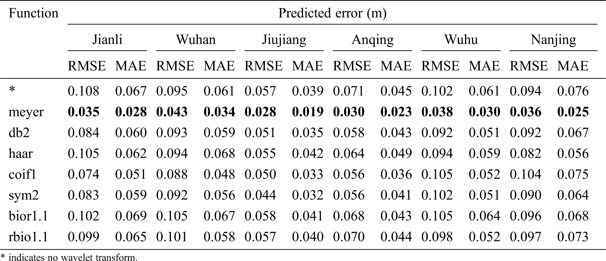
Table 8: Comparisons of the Meyer wavelet decomposition levels in optimal prediction steps
5.4 Comparison with Prediction Models
In order to confirm the effectiveness and generalization of the WA-LSTM model, comparison experiments are carried out using the state-of-the-art prediction models, such as ANN, LSTM and ARIMA, these models are also combined with Meyer wavelet transform at level 4, their prediction structures are the same in Fig. 1. Without loss of generality, each experiment repeats thirty times. According to Tab. 9, the WA-LSTM model always has the minimum RMSE and MAE compared with other models, which is 46%, 51%, 39%, 50%, 74%, 72% better than the LSTM on RMSE at Jianli, Wuhan, Jiujiang, Anqing, Wuhu, Nanjing, respectively, and 31%, 37%, 19%, 30%, 53%, 50% better than the WA-ANN, as well as 86%, 74%, 61%, 63%, 79%, 92% better than the WA-ARIMA. The box and whisker plots of the results in Fig. 5 are also help graphically compare the distributions. Apparently, the proposed WA-LSTM model is demonstrated to be more effective and promising for water level prediction in practice than other models.
Table 9: Comparisons of the state-of-the-art models
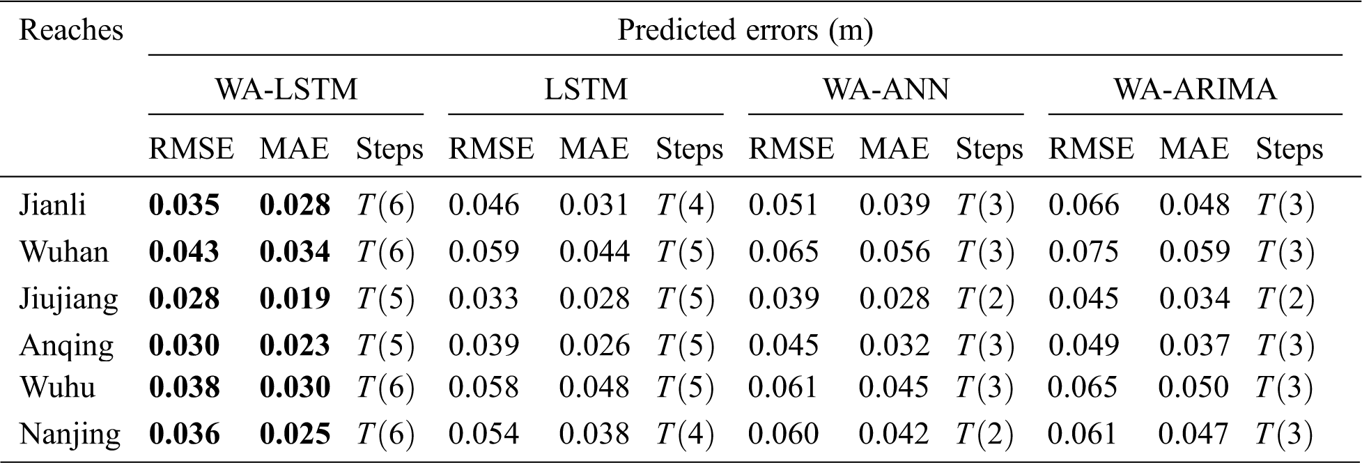

Figure 5: The box and whisker plots performances of the state-of-the-art models on RMSE. (a) Jianli, (b) Wuhan, (c) Jiujiang, (d) Anqing, (e) Wuhu, (f) Nanjing
In this research, a new WA-LSTM model based on discrete wavelet transform and long short-term memory network for water level prediction in Yangtze River is proposed to help flood control and vessel navigation. In the provided model, water level time series are firstly decomposed into high frequency and low frequency components using wavelet transforms with different scales for a better understanding of temporal properties, then each component is put into the LSTM network for independent prediction, finally, the predicted values are reconstructed to get the predicted water level in one day ahead.
In order to confirm the effectiveness and generalization of the model, six representative reaches including Jianli, Wuhan, Jiujiang, Anqing, Wuhu and Nanjing are applied to study, and several comparisons are developed, including the practicable of temporal and spatial combination, the sensitivity of mother wavelet types and decomposition levels, the efficiency of the state-of-the-art models contained LSTM, WA-ANN and WA-ARIMA. Comprehensive research finds out that 5 or 6 days lag observations as input features using Meyer wavelet transform with decomposition level 4 provides the best performance, which less than 0.045 m on RMSE and less than 0.035 m on MAE in general, extraordinary has only 0.028 m on RMSE and 0.019 m on MAE at Jiujiang reaches. The results are superior to those of competing models, and demonstrates that the WA-LSTM model has strong applicability and generalization, provides references to further research on water level prediction in Yangtze River.
Future research would look into more comprehensive prediction that incorporates with the temporal characteristics like dry season and flood season, or the weather forecasting such as rainstorm, or the waterway tributary characteristics. Furthermore, it would be interesting to investigate other deep learning models for water level prediction.
Acknowledgement: The authors are very thankful to the Changjiang Maritime Safety Administration for the availability of the data resources.
Funding Statement: The authors received no specific funding for this study.
Conflicts of Interest: The authors declare that they have no conflicts of interest to report regarding the present study.
1. H. Q. Hou, X. L. Liu, W. X. Xu and H. H. Liu. (2015). “Short-term water level prediction in middle stream of Yangtze River,” Advanced Materials Research, vol. 1065, no. 1, pp. 2983–2988. [Google Scholar]
2. S. D. Xu and W. Huang. (2011). “Estimating extreme water levels with long-term data by GEV distribution at Wusong station near Shanghai city in Yangtze Estuary,” Ocean Engineering, vol. 38, no. 2, pp. 468–478. [Google Scholar]
3. Y. H. Cao, X. F. Ye and G. H. Lv. (2012). “Study on water level prediction in the Ganjiang Valley,” Applied Mechanics & Materials, vol. 212, no. 10, pp. 417–422. [Google Scholar]
4. G. F. Li, X. Y. Xiang, J. Wu and Y. Tan. (2013). “Long-term water-level forecasting and real-time correction models in the tidal reach of the Yangtze River,” Journal of Hydrologic Engineering, vol. 18, no. 11, pp. 1437–1442. [Google Scholar]
5. Q. Zhang, C. L. Liu, C. Y. Xu, Y. P. Xu and T. Jiang. (2006). “Observed trends of annual maximum water level and streamflow during past 130 years in the Yangtze River basin, China,” Journal of Hydrology, vol. 324, no. 1, pp. 255–265. [Google Scholar]
6. T. Liu, P. L. Zhang and Y. Xu. (2014). “Research on water level trends of the middle Yangtze River based on Mann-Kendall and ARIMA model,” Applied Mechanics & Materials, vol. 513, no. 2, pp. 3016–3019. [Google Scholar]
7. C. W. Dawso, R. L. Wilby, C. Harpham and Y. Chen. (2002). “Evaluation of artificial neural network techniques for flow forecasting in the river Yangtze,” China Hydrology and Earth System Sciences, vol. 6, no. 4, pp. 619–626. [Google Scholar]
8. J. Zheng. (2014). “Analysis of the Three Gorges Reservoir operation on the water level of Yangtze River during the non-flood season,” Advanced Materials Research, vol. 864, no. 3, pp. 2207–2212. [Google Scholar]
9. J. X. Liu, J. Y. Deng, Y. F. Chai, Y. P. Yang and S. X. Li. (2019). “Variation of the water level in the Yangtze River in response to natural and anthropogenic changes,” Water, vol. 11, no. 12, pp. 2594. [Google Scholar]
10. C. Mattia, M. Paolo, D. G. Ludovica, N. Claudia, P. Luca et al. (2015). , “Seasonal river discharge forecasting using support vector regression: A case study in the Italian Alps,” Water, vol. 7, no. 5, pp. 2494–2515. [Google Scholar]
11. A. Mirarabi, H. R. Nassery, M. Nakhaei, J. Adamowski and A. H. Akbarzadeh. (2019). “Evaluation of data-driven models (SVR and ANN) for groundwater level prediction in confined and unconfined systems,” Environmental Geology, vol. 78, no. 15, pp. 489.1–489.15. [Google Scholar]
12. B. Bunchingiv, G. Hildebrandt and K. P. Holz. (2003). “Short-term water level prediction using neural networks and neuro-fuzzy approach,” Neurocomputing, vol. 55, no. 3, pp. 439–450. [Google Scholar]
13. R. Adnan, F. A. Ruslan, A. M. Samad and Z. M. Zain. (2012). “Artificial neural network modelling and flood water level prediction using extended Kalman filter,” in IEEE Int. Conf. on Control System, Computing and Engineering, ICCSCE, Penang, Malaysia, pp. 535–538. [Google Scholar]
14. M. Y. A. Khan, F. Hasan, S. Panwar and G. J. Chakrapani. (2016). “Neural network model for discharge and water-level prediction for Ramganga River catchment of Ganga Basin,” India Hydrological Sciences Journal, vol. 61, no. 11, pp. 2084–2095. [Google Scholar]
15. M. Rezaeianzadeh, L. Kalin and C. J. Anderson. (2017). “Wetland water-level prediction using ANN in conjunction with base-flow recession analysis,” Journal of Hydrologic Engineering, vol. 22, no. 1, pp. 1–11. [Google Scholar]
16. D. N. Fabio and G. Francesco. (2020). “Groundwater level prediction in Apulia region (Southern Italy) using NARX neural network,” Environmental Research, vol. 190, no. 8, pp. 110062. [Google Scholar]
17. C. Choi, J. Kim, H. Han, D. Han and H. S. Kim. (2019). “Development of water level prediction models using machine learning in Wetlands: A case study of Upo Wetland in South Korea,” Water, vol. 12, no. 1, pp. 93. [Google Scholar]
18. M. R. Zadeh, H. Tabari and H. Abghari. (2013). “Prediction of monthly discharge volume by different artificial neural network algorithms in semi-arid regions,” Arabian Journal of Geosciences, vol. 7, no. 6, pp. 2529–2537. [Google Scholar]
19. T. Partal. (2009). “River flow forecasting using different artificial neural network algorithms and wavelet transform,” Revue Canadienne De Génie Civil, vol. 36, no. 1, pp. 26–38. [Google Scholar]
20. A. D. Mehr, E. Kahya, A. Ahin and M. J. Nazemosadat. (2015). “Successive-station monthly streamflow prediction using different artificial neural network algorithms,” International Journal of Environmental Science & Technology, vol. 12, no. 7, pp. 2191–2200. [Google Scholar]
21. X. Y. Chen, K. W. Chau and A. O. Busari. (2015). “A comparative study of population-based optimization algorithms for downstream river flow forecasting by a hybrid neural network model,” Engineering Applications of Artificial Intelligence, vol. 46, no. 10, pp. 258–268. [Google Scholar]
22. M. Das, S. K. Ghosh, V. M. Chowdary, A. Saikrishnaveni and R. K. Sharma. (2016). “A probabilistic nonlinear model for forecasting daily water level in reservoir,” Water Resources Management, vol. 30, no. 9, pp. 3107–3122. [Google Scholar]
23. F. J. Chang and Y. T. Chang. (2006). “Adaptive neuro-fuzzy inference system for prediction of water level in reservoir, Advances in Water Resources,” Advances in Water Resources, vol. 29, no. 1, pp. 1–10. [Google Scholar]
24. A. Altunkaynak and E. Kartal. (2019). “Performance comparison of continuous wavelet-fuzzy and discrete wavelet-fuzzy models for water level predictions at northern and southern boundary of Bosphorus,” Ocean Engineering, vol. 186, no. 10, pp. 258–268. [Google Scholar]
25. B. Wang, B. Wang, W. Z. Wu, C. B. Xi and J. C. Wang. (2020). “Sea-water-level prediction via combined wavelet decomposition, neuro-fuzzy and neural networks using SLA and wind information,” Acta Oceanologica Sinica, vol. 39, no. 5, pp. 161–171. [Google Scholar]
26. M. Jayalakshmi and S. N. Rao. (2020). “Discrete wavelet transmission and modified PSO with ACO based feed forward neural network model for brain tumour detection,” Computers Materials & Continua, vol. 65, no. 2, pp. 1081–1096. [Google Scholar]
27. N. Jayashree and R. S. Bhuvaneswaran. (2019). “A robust image watermarking scheme using z-transform, discrete wavelet transform and bidiagonal singular value decomposition,” Computers Materials & Continua, vol. 58, no. 1, pp. 263–285. [Google Scholar]
28. G. Hinton, S. Osindero and Y. W. Teh. (2006). “A fast learning algorithm for deep belief nets,” Neural Computation, vol. 18, no. 8, pp. 1527–1554. [Google Scholar]
29. B. D. Oh, H. J. Song, J. D. Kim, C. Y. Park and Y. S. Kim. (2019). “Predicting concentration of PM10 using optimal parameters of deep neural network,” Intelligent Automation & Soft Computing, vol. 25, no. 2, pp. 343–350. [Google Scholar]
30. S. Hochreiter and J. Schmidhuber. (1997). “Long short-term memory,” Neural Computation, vol. 9, no. 8, pp. 1735–1780. [Google Scholar]
31. C. H. Yang, C. H. Wu and C. M. Hsieh. (2020). “Long short-term memory recurrent neural network for tidal level forecasting,” IEEE Access, vol. 8, pp. 159389–159401. [Google Scholar]
32. N. Pan, Y. Liu, D. Pan, J. Qian and G. Li. (2019). “Line trace effective comparison algorithm based on wavelet domain DTW,” Intelligent Automation & Soft Computing, vol. 25, no. 2, pp. 359–366. [Google Scholar]
33. Z. Guo, L. Zhang, X. Hu and H. Chen. (2020). “Wind speed prediction modeling based on the wavelet neural network,” Intelligent Automation & Soft Computing, vol. 26, no. 3, pp. 625–630. [Google Scholar]
34. V. Moosavi, M. Vafakhah, B. Shirmohammadi and N. Behnia. (2013). “A wavelet-ANFIS hybrid model for groundwater level forecasting for different prediction periods,” Water Resources Management, vol. 27, no. 5, pp. 1301–1321. [Google Scholar]
 | This work is licensed under a Creative Commons Attribution 4.0 International License, which permits unrestricted use, distribution, and reproduction in any medium, provided the original work is properly cited. |