DOI:10.32604/iasc.2021.016415
| Intelligent Automation & Soft Computing DOI:10.32604/iasc.2021.016415 | |
| Article |
Tomato Leaf Disease Identification and Detection Based on Deep Convolutional Neural Network
1Department of Electronics and Information Engineering, Tongji University, Shanghai, 201804, China
2BEACON Center for the study of Evolution in Action, Michigan State University, East Lansing, MI 48824, USA
*Corresponding Author: Lihong Xu. Email: wu_tim@tongji.edu.cn
Received: 01 January 2021; Accepted: 26 February 2021
Abstract: Deep convolutional neural network (DCNN) requires a lot of data for training, but there has always been data vacuum in agriculture, making it difficult to label all existing data accurately. Therefore, a lightweight tomato leaf disease identification network supported by Variational auto-Encoder (VAE) is proposed to improve the accuracy of crop leaf disease identification. In the lightweight network, multi-scale convolution can expand the network width, enrich the extracted features, and reduce model parameters such as deep separable convolution. VAE makes full use of a large amount of unlabeled data to achieve unsupervised learning, and then uses labeled data for supervised disease identification. However, in the actual model deployment and production environment, VAE doesn’t require additional calculation and storage consumption, because it is not used in the calculation of the application phase. Compared with the classification network that only uses labeled data, the generalization effect and identification accuracy of this proposed method are enhanced. Especially in the case of fewer labeled samples, the identification accuracy has increased from 56.13% to 78.03%, and in the case of many labeled samples, the identification accuracy also shows a rise. We have fully confirmed the effectiveness of the lightweight network and VAE enhancement strategy: the correct detection rate of disease category by this method is 94.17%, and only 0.42% of the diseased leaves are misidentified as healthy leaves; the correct detection rate of healthy leaves is 98.27%, and only 1.73% of healthy leaves are misidentified as diseased leaves.
Keywords: CNN; VAE; leaf diseases; identification; detection
According to Food and Agriculture Organization of the United Nations (FAO), pests and diseases can cause $70 to $90 billion annual losses worldwide. China is no exception. In 2018, crop diseases affected an area of about 100 million mu (13.34 hectares), causing nearly 8% loss in China's agricultural output. Timely and accurate identification of diseases is the key to right treatment [1], and an important prerequisite for reducing crop loss and pesticide use.
Precision agriculture is an effective way to achieve sustainable development of agriculture with high quality, high yield, low consumption and environmental protection. Disease diagnosis is an important part of precision agriculture. In recent years, neural network technology has been widely used in classification and identification [2–6]. Unlike plant classification and identification, disease identification is more difficult. Plants can generally be identified by the shape of leaves and flowers [7]. However, the occurrence, development and spread of diseases can cause huge difference in leaf phenotypic characteristics, which can make disease identification difficult. Since 1950s, scholars have carried out research on crop disease identification based on image processing technology [8,9]. Brahimi et al. [10] fine-tuned the network parameters of AlexNet, and classified and identified plant diseased leaves [11]. Such fine-tuning methods enjoy higher accuracy than support vector machine (SVM), and can avoid the influence of disease spot segmentation on recognition. Wu et al. [12] used weak supervision to segment tomato leaves, and then applied neural network to classify leaf diseases. Khamparia et al. [13] applied convolutional neural network (CNN) and auto-encoder to detect crop diseases by using crop leaf images with the help of convolutional encoder network. Sun et al. [14] used CNN to improve the identification efficiency of tea diseases through image segmentation and data enhancement.
In view of the above problems, we propose a method to improve the accuracy of tomato leaf disease identification by applying the lightweight network and VAE to the detection network. Multi-scale convolution is used to expand the network width, which makes the extracted features more abundant; deep separable convolution is used to reduce model parameters to meet the needs of low-cost terminals. In the identification network, VAE makes full use of a large amount of unlabeled data to realize unsupervised learning, and then uses labeled data to perform supervised disease identification. In the detection network, the training results of feature extraction of the identification network are used as initial parameters of the “backbone” network for detection and segmentation training. In the detection and identification of tomato leaf diseases, both labeled and unlabeled data are fully utilized to improve identification accuracy. In this paper, tomato leaf disease identification is used as an example, and we hope the technology can be used in identifying similar crop leaf diseases.
PlantVillage is an internet image library of plant leaf diseases initiated and established by epidemiologist David [15] to diagnose plant disease using machine learning technology. The dataset collected more than 50,000 images of visible light leaves from 38 types of 14 plants, including 12 healthy leaves and 26 diseased leaves. Among them, 18,160 tomato leaves, including healthy leaves and 9 diseased leaves, are used as the crop disease classification dataset for this experiment. Fig. 1 shows an example of 10 tomato leaf images in the dataset. No.1-No.10 are healthy, tomato bacterial spot, early blight, late blight, leaf mold, mosaic virus, septoria leaf spot, target spot, two-spotted spider mite and yellow leaf curl virus leaves, respectively.
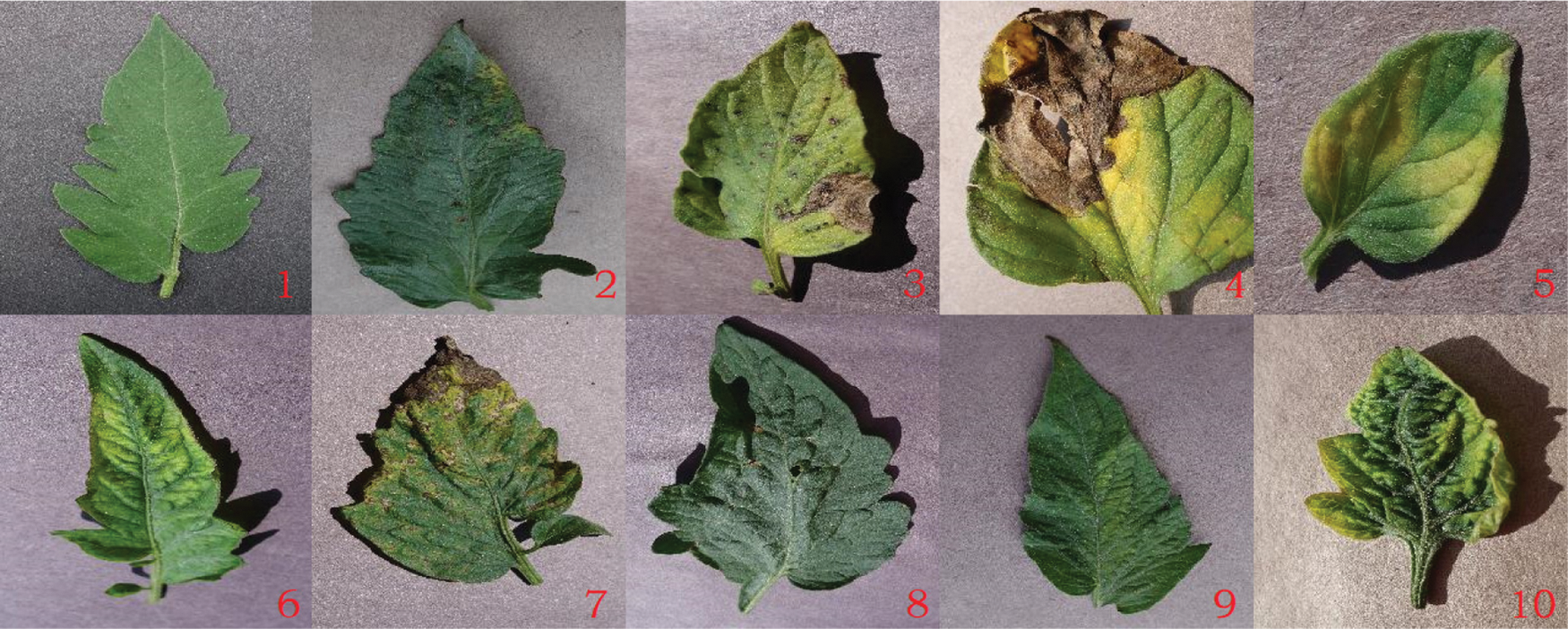
Figure 1: Image of 10 kinds of tomato leaves
We collected images of real tomato leaves for training and testing to verify the effectiveness of the method. The images include 186 diseased leaves and 463 healthy leaves. There are 5 diseases in the leaf images. As shown in the first row of Figs. 2a–2g are healthy, tomato bacterial spot, early blight, early blight, late blight, leaf mold, septoria leaf spot leaves, respectively. The above images are original, and the bottom images are the annotation after pre-processed. The photos of these healthy tomato leaves are taken in a glass greenhouse in the Chongming base of the China National Center for Facilities and Agricultural Engineering and Technology Research.
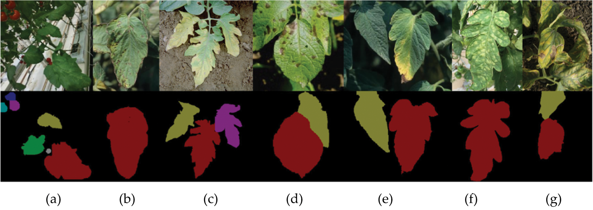
Figure 2: Images of tomato leaves in real scene
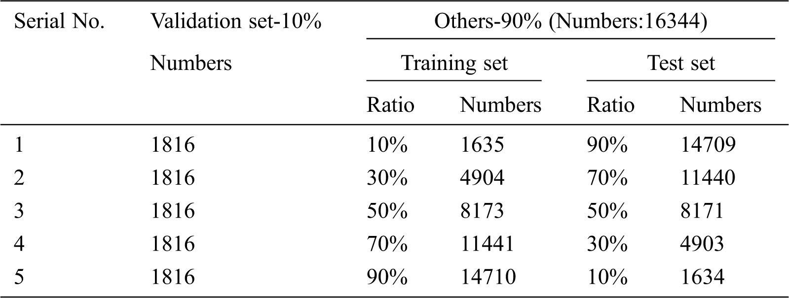
In order to reduce computation, the size of the 10 tomato images in the PlantVillage dataset is normalized to 128*128 pixels. Then 10% of the images are randomly divided into verification sets, and the remaining samples of each category are divided into five groups according to the proportion respectively, to train the model in different situations and evaluate the performance of the model. The proportions of the training set-validation set are 10%–90%, 30%–70%, 50%–50%, 70%–30% and 90%–10% respectively, there are five cases of simulated training set with little, less, half, more and many to verify the effectiveness of the method under different conditions. The sample amount of each set is shown in Tab. 1.
Table 1: Different partitioning of dataset
2.2 Tomato Leaf Disease Identification Model
Convolutional neural network (CNN), a feedforward neural network with deep structure, has become the first solution of image classification. Common CNNs include AlexNet [11], VggNet [16], ResNet [17] and Inception [18]. CNN can extract features of different semantic levels of images. As the number of network layers increases, the extracted features become more and more abundant. However, when the network reaches a certain depth, it is difficult to find the optimal weight parameters during the training process, resulting in a “degradation” with large errors. To this end, He et al. [17] proposed residual neural network to achieve higher accuracy. For crop disease identification, the support of high-performance workstation may be lacking in general practical applications, and too deep network will increase the difficulty of model training. Moreover, the trained model has a greater demand for memory, and it is difficult to meet the requirements of low-cost terminals. Accelerate network model design that is mainly to explore the optimal network structure, can achieve a similar effect while reducing calculation, usually by group convolution, decomposition convolution [19], Bottleneck structure [17], SqueezeNet structure [20], etc.
Fig. 3a shows an example of using deep neural network to identify tomato leaf diseases. The input is an image of a tomato leaves, and the output is the corresponding disease category. Deep neural network is a machine learning model with deep supervised learning based on data. The Class Network in the figure is composed of CNN, and can be divided into two parts, as shown in Fig. 3b. The former is used to extract features, and the latter is used to classify features through fully connection.
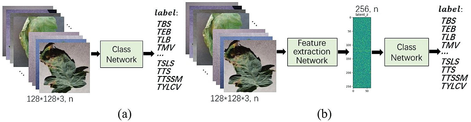
Figure 3: (a) leaf disease identification model, (b) identification model shown separately
2.2.1 Leaf Disease Identification Networks
The lightweight neural network is mainly composed of 5 stages and 4 reduction layers, include Stage1-5, Reduction1-4, Max-pooling, FC, Dropout, FC-10 and Softmax. Stage1 consists of three 3*3 convolution stages, and the stride of the first convolution is 2. Stage2 and Stage3 are composed of two module1 connected in series respectively. Stage4 and Stage5 include two module2 connected in series. Reduction1-4 are reduction modules, which are used to reduce the image size and expand channels in place of common pooling operations. Reduction module uses group convolution and channel shuffle instead of standard convolution operations. Finally, through the fully connected layer (FC), the Dropout [21] layer and Softmax, 10 kinds of recognition results can be obtained. The overall framework of the improved network is shown in Fig. 4.
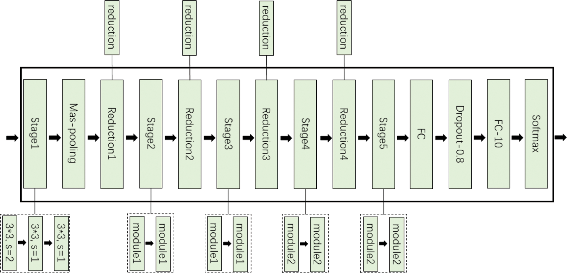
Figure 4: Tomato leaf disease diagnosis network framework
2.2.2 Component Module of Disease Diagnosis Networks
Group convolution is an effective sparse connection method, which can divide the input feature map into different groups along the channel dimension, and then perform convolution operations on different groups respectively. MobileNet [22] uses depth separable convolution to build a lightweight depth neural network. The standard convolution is decomposed into depthwise convolution and pointwise convolution. Depthwise convolution, as an extreme of group convolution, can be regarded as group convolution with only one channel in each group. Pointwise convolution uses 1*1 convolution with low overhead to combine the information of each channel for channel fusion, which can greatly reduce the number of parameters and computation. At the lower level of the network, the standard convolution of 3*3 in multi-scale residual module is replaced by the depth separable convolution to obtain the lightweight multi-scale residual learning module, as shown in Fig. 5a, which is module1 in Fig. 4. Where, conv/dw and conv/pw respectively represent depthwise convolution and pointwise convolution, which constitute the depth separable convolution.
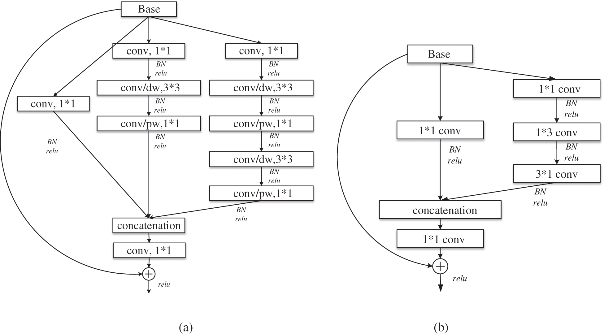
Figure 5: Lightweight residual module: (a) module1; (b) module2
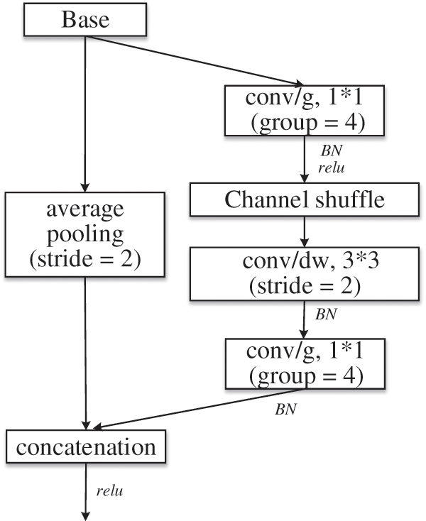
Figure 6: Reduction module: reduction
As the number of network layers increases, the receptive field becomes larger, the features become abstract, the number of channels increases, and the number of convolution kernels increases. Therefore, the use of large convolution kernel will inevitably bring more parameters. So, in the deeper layer of the network, large convolution kernel is removed to reduce parameters. In addition, factorizing convolution [19] decomposes the convolution of k*k into 1*k and k*1 to reduce the complexity of the calculation, as shown in Fig. 5b, which is module2 in Fig. 4.
Group convolution is troubled by “poor information flow”, and thus ShuffleNet [23] adopts channel shuffle to solve this problem. A novel feature map is constructed by shuffling the channels of the convolutional feature map. That is, each conv/g is part of the output channel. When the group convolution is shuffled and recombined, information is exchanged between channels. Therefore, the reduction module shown in Fig. 6 is adopted to replace the pooling operation that is commonly used to reduce image size and expand channels. Where, conv/g represents group convolution, divided into 4 groups, and the size of convolution kernel is 1*1.
2.3 Improve the Identification Accuracy by Variational auto-Encoder
2.3.1 Variational Auto-Encoder
Variational auto-Encoder (VAE) [24] is a generative model based on variational bayes proposed by Diederik P. Kingma and Max Welling. VAE encodes the mode into the multivariate normal distribution of the latent space through encoder, and then reconstructs the image from the latent space through decoder. VAE can map images from pixel space to normal distribution space, and all images will be encoded into two vectors of size n, where n is the specified hyperparameter of the latent space. In practice, we can use CNN to implement VAE.
2.3.2 VAE Enhance Identification of Tomato Leaf Diseases
Compared with other commonly used classifications, crop disease identification is more professional that requires more experience. In actual research, some disease images are accurately labeled whereas most disease images are not. For this reason, VAE is used to improve the classification accuracy of tomato leaf disease identification model based on deep neural network. VAE includes two steps. The first step is to train the VAE Network to obtain the Encoder Network parameters, and the second step is to train the Classification Network to realize the classification function. The network structure is shown in Fig. 7 in blue box and red box respectively. The Classification Network is composed of two parts as shown in Fig. 3b. The first part is used to extract features, and the second part is to combine features to determine the category. It should be noted that our goal is to strengthen the learning of Classification Network and improve the identification accuracy. The introduced VAE Network does not participate in test and application, but only participates in the training. Therefore, no additional calculation and storage consumption will be introduced in the actual model deployment and production environment. In addition, Gaussian sampling is used in VAE Network and Classification Network, which not only generates codes, but also adds noise. Thus, it can enhance the generalization effect of the model and reduce overfitting.
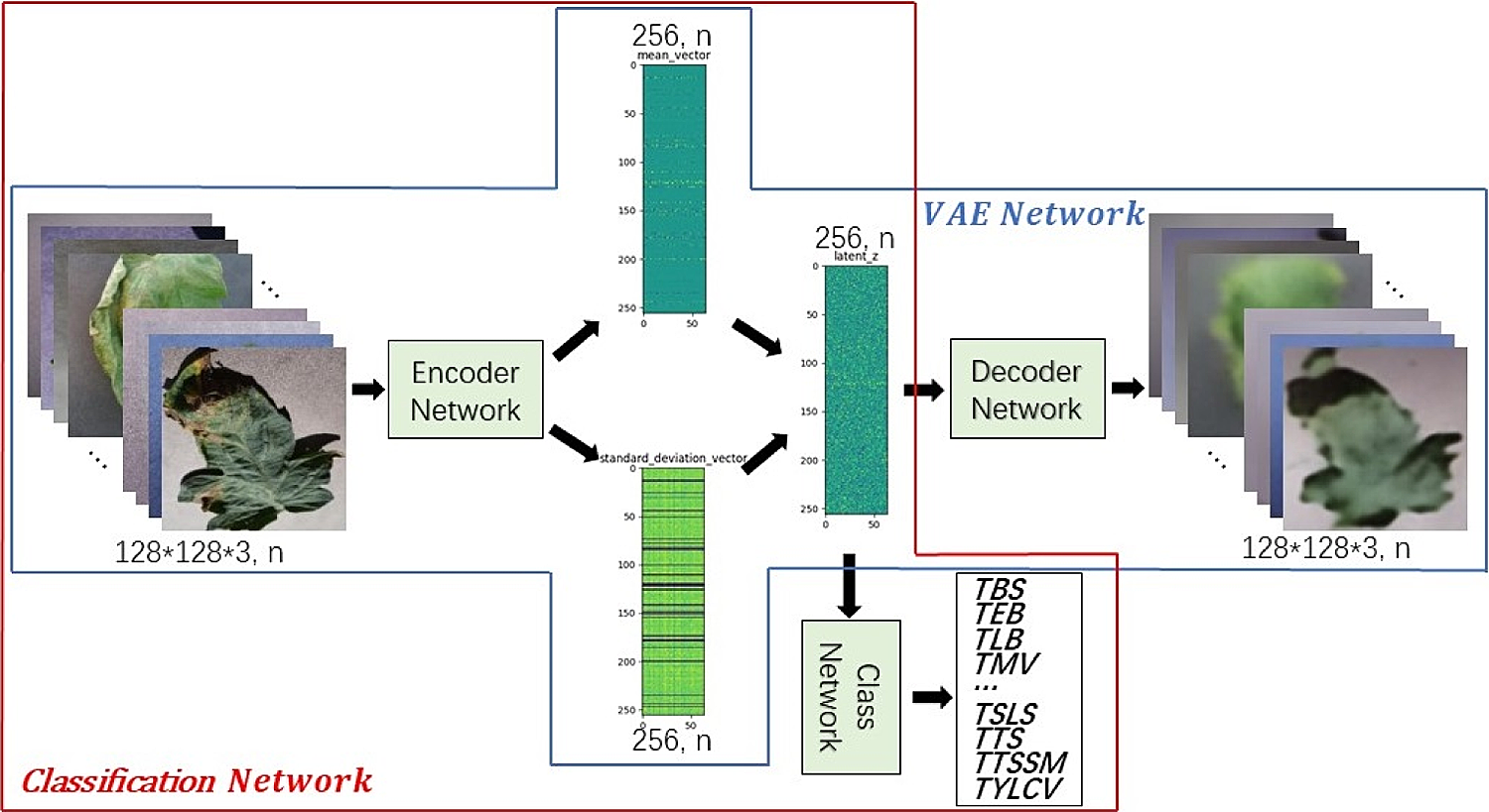
Figure 7: VAE enhance identification of tomato leaf diseases
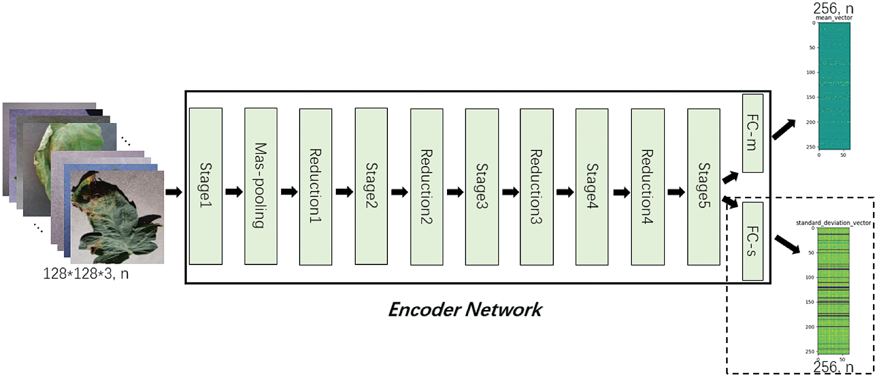
Figure 8: Encoder Network
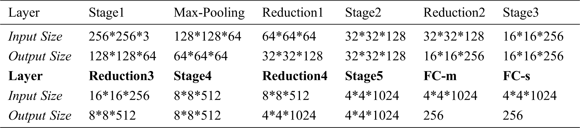
Lightweight tomato leaf disease identification network shown in Fig. 3 is divided into two parts of “Encoder Network” and “Class Network, with the addition of ”Decoder Network”, form similar to Fig. 7, specific as follows, “Encoder Network” contains StageX(X=1,2,…,5), ReductionX(X=1,2,…,4), Max-pooling, FC-m, FC-s structure, the input is a tomato leaf images, the output is a two-dimensional vector with length of 256, as shown in Fig. 8. Tab. 2 shows the output sizes of each layer in Encoder Network.
Table 2: Input and output dimensions of each layer of the Encoder Network
Decoder Network includes FC-4096, UpsampleX(X=1,2,…,6), ScaleX(X=1,2,…,6) and Conv3-3 structures, the input is a latent vector of length 256, and the output is the reconstructed image with size of 128*128*3, as shown in Fig. 9. Tab. 3 shows the output size of each layer in Decoder Network.
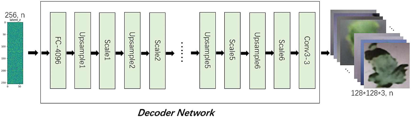
Figure 9: Decoder network
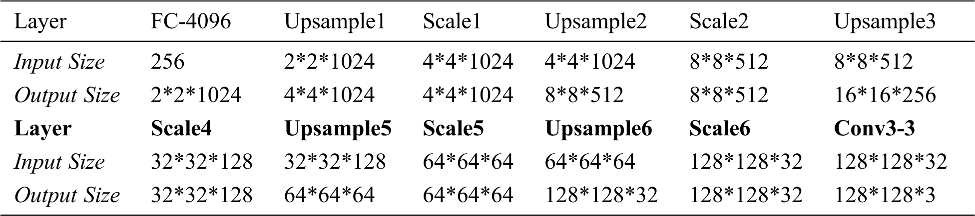
In Decoder Network, FC-4096 changes the length of latent vector from 256 to 4096 through the fully connected layer, and then changes the shape to 2*2*1024. UpsampleX uses a 3*3 convolution kernel to perform the expansion convolution, so as to realize the expansion of the input size and the transformation of channel number. ScaleX is a “building block” in Resnet structure consisting of two 3*3 convolution and shortcut, with the same input and output dimensions. Conv3-3 uses a 3*3 convolution kernel to extract the features, reducing the channel from 32 to 3.
Table 3: Input and output dimensions of each layer of the Decoder Network
Classification Network is divided into Encoder Network and Class Network. Encoder network is part of the VAE network. Class Network mainly maps the features learned by Encoder Network to class labels, which are composed of Dropout, FC-10 and Softmax. During the training, Dropout randomly eliminates some neurons with a certain probability, so that the corresponding parameters are not updated in the process of back propagation. The FC-10 layer changes the size of the output feature vector to 10 through fully connection, which corresponds to the category of tomato leaf disease identification task. The Softmax layer maps the output of multiple neurons to the (0,1) interval which can be understood as a probability for multiple classification.
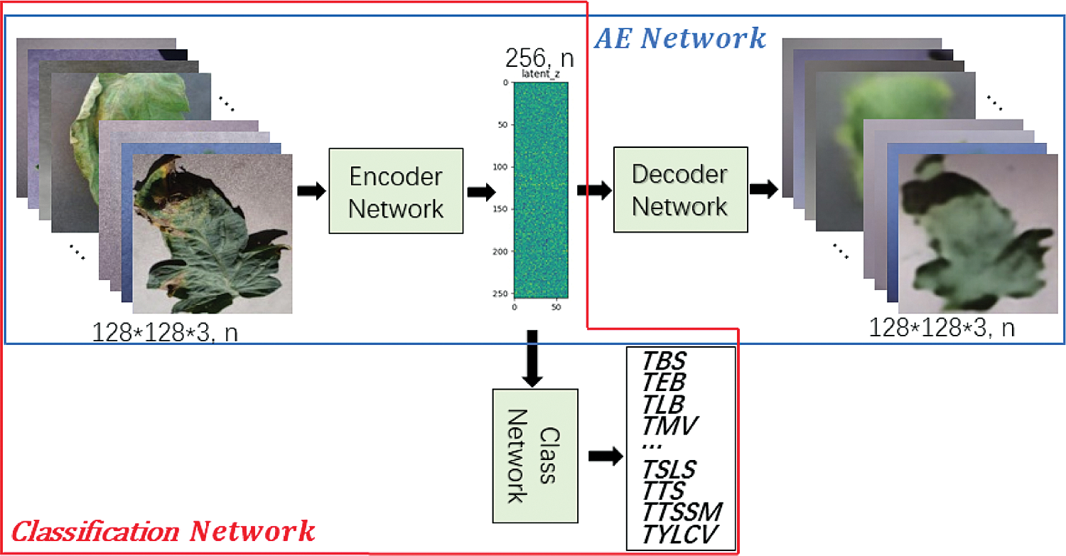
Figure 10: AE enhanced identification of tomato leaf diseases
In this paper, we propose four methods for comparison, namely “Class”, “AE-Class”, “Class-z” and “VAE-Class-z”. “Class” represents “Classification Network” in red box shown in Fig. 10. In the implementation, the lightweight tomato leaf disease identification network is shown in Fig. 3. “AE-Class” includes the structure of “AE Network” in blue box and “Classification Network” in red box shown in Fig. 10. That is, the Decoder network shown in Fig. 9 is added to the classification network shown in Fig. 3. The reconstruction model auto-encoder (AE) network [24] is first trained with all data (including labeled data and unlabeled data), and then Classification Network is trained with labeled data only. “Class-z” only includes the “Classification Network” shown in Fig. 7. Compared with “Class”, the latent vector z of “Class-z”, being sampled from Gaussian distribution, can increase uncertainty, rather than directly classify the features extracted from the input data. “VAE-Class-z” stands for the structure shown in Fig. 7, including the VAE Network and Classification Network. It first trains the model VAE Network with all data, and then the Classification Network with labeled samples. Compared with “VAE-Class-z”, “AE-Class” uses directly generated features instead of sampled features for training and classification.
2.4 Tomato Leaf Disease Detection Model
There are two common solutions for target detection tasks. One is two-stage target detection, and the other is one-stage target detection. In two-stage target detection, the target is recognized through a neural network before classification, whereas in one-stage target detection, the network is used directly to detect the target. Two-stage target detection is easy to implement, but the downstream classification depends on the performance of the upstream identification and positioning. However, although one-stage target detection does not need to identify the target first, it makes end-to-end target detection more difficult to achieve. In summary, the two-stage method has higher accuracy but lower speed compared to the one-stage method. When detecting tomato diseases, the speed of the two-stage method can meet the requirements of higher precision, such as Faster R-CNN [25]. We propose to use Mask R-CNN [26] to enhance the performance of Faster R-CNN on bounding box recognition by adding object mask branch in parallel to existing branches, as shown in Fig. 11. Mask R-CNN is used for object instance segmentation. Instance segmentation algorithms usually require an accurate pixel-level segmentation mask to monitor labels to be assigned to all the training samples. However, collecting labels is difficult, and labeling a new category takes time and effort. Therefore, weakly supervised method [12] is adopted to mark the leaf pixels and disease types in the training stage.
The identification accuracy of the detection model is improved based on deep neural network. It is implemented by following two steps. Firstly, lightweight tomato leaf disease identification network based on VAE (VAE-Class-z) is trained and parameters of Encoder Network are obtained. Secondly, the trained Encoder Network is used as the “backbone” network of Mask R-CNN to train the model with the segmentation data of diseased leaves. In actual use, only the Mask R-CNN network is involved in the test phase. Therefore, no additional calculation and storage consumption is introduced in the actual model deployment and production environment.
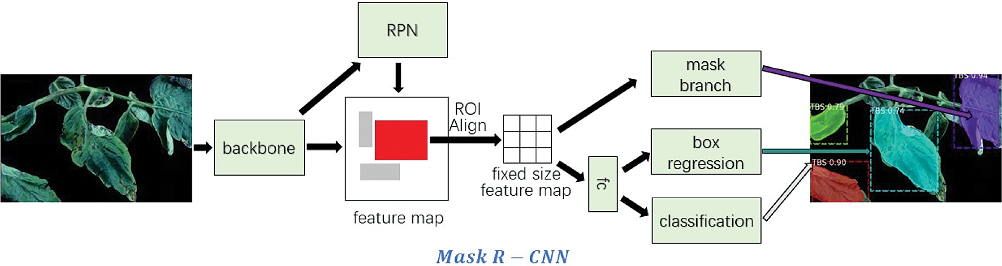
Figure 11: Mask R-CNN
The experimental configuration environment of this paper is as follows: Ubuntu16.04 LST 64-bit system, processor Intel Core i5-8400(2.80 GHz), memory is 8 GB, graphics card is GeForce GTX1060 (6G), using Tensorflow-GPU1.4 deep learning framework, using Python programming language. The same training parameters are used in the experiment. For example, the size of the generated latent vector is 256, the epoch is 20, and the Adam optimizer is used to solve the minimum loss.
3.2 Comparison of Different Depth Model Identification Indicators
Table 4: Comparison of different depth model recognition indexes
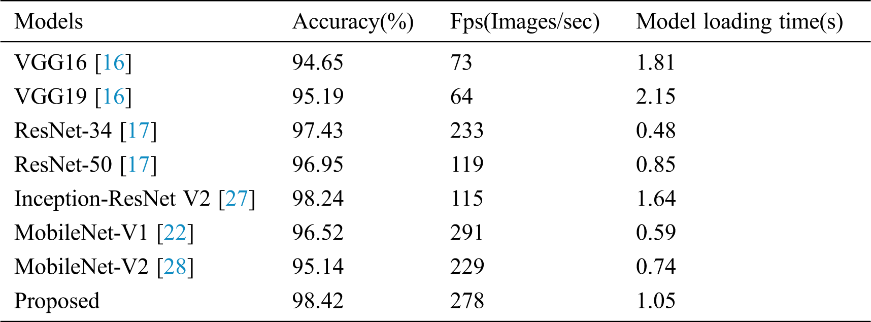
The improved convolutional neural network is compared with several advanced convolutional neural networks, including VGG16/19, ResNet-34/50, Inception-ResNet-V2, MobileNet-V1/V2 in diagnosing and identifying tomato diseased leaves. Tab. 4 lists the classification accuracy and the model size after training under different neural network models. In this part, Serial No.5 in Tab. 1 is used to test the improved model.
It can be seen from Tab. 4 that the improved neural network model can achieve 98.42% accuracy. Compared with the traditional convolutional network model, the proposed network model has higher accuracy, which shows the effectiveness of using multi-scale convolution in the residual module to improve network performance. In addition, the number of parameters in the model is also significantly reduced.
3.3 Analysis of Classification Results
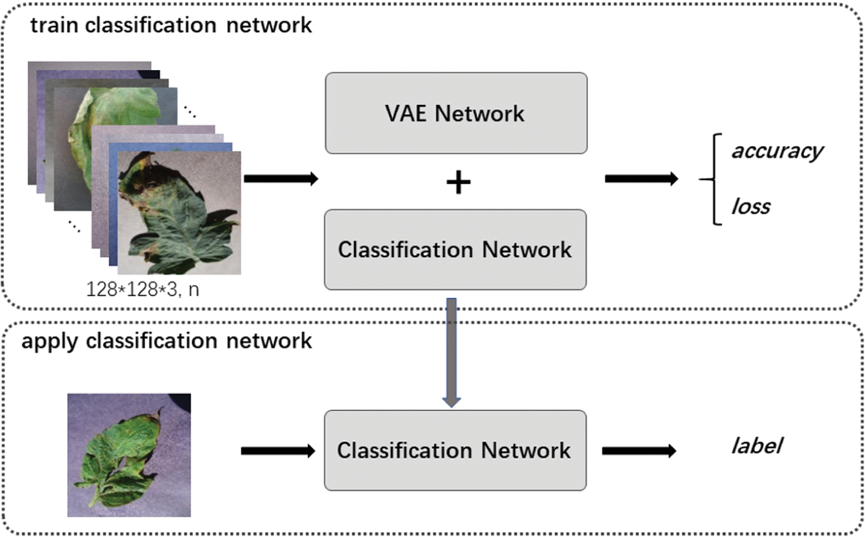
Figure 12: Framework of classification network by VAE enhancement strategy
Fig. 12 shows the framework of classification network. It includes two stages: train classification network and apply classification network. For training, firstly, we use labeled and unlabeled data to train “VAE Network”, and then only use labeled data to train “Classification Network”. In application, we only use the trained “Classification Network” to identify the labels of the input images.
In order to verify the usability of the identification model in different senarios, according to the proportion of training sets and validation sets, the dataset is divided into 5 groups. As shown in Tab. 1, the proportion of training set-verification set of Serial No.1-5 corresponding to 5 samples, respectively.
In Fig. 13a–13e correspond to the classification loss of four methods in 5 different samples, and (f) corresponds to the classification accuracy of four methods in 5 samples. As mentioned above, these four methods are Class, AE-Class, Class-z, VAE-Class-z respectively. It can be seen from Fig. 13, the loss of Class and Class-z is larger than the two enhancement methods, and the loss decreases slowly, indicating that the unlabeled data enhancement method makes the loss smaller and decreases rapidly.
As shown in Fig. 13f, the diagram of VAE-Class-z corresponding classification accuracy is the highest in the five sets of data. It shows that VAE enhancement method can significantly improve the classification accuracy of the network, especially in the case of fewer samples (such as Serial No.1), where the identification accuracy increased to 78.03% in VAE-Class-z from 56.13% in Class. And in the case of more labeled samples (such as Serial No. 5), the identification accuracy increased to 98.87% in VAE-Class-z from 98.42% in Class, showing an increase of 0.45%. By comparing Class and Class-z, when the amount of labeled samples is small (Serial No.1), the increase in model uncertainty can reduce the accuracy; when the number of labeled samples is large (Serial No.4-5), the increase of uncertainty in the model can slightly improve accuracy. Both AE-Class and VAE-Class-z can significantly increase the classification accuracy, and the VAE-Class-z method is better. This is because although Gaussian sampling increases the uncertainty, the model can learn this uncertainty with VAE-Class-z enhancement, thus enhancing the generalization effect of the model.
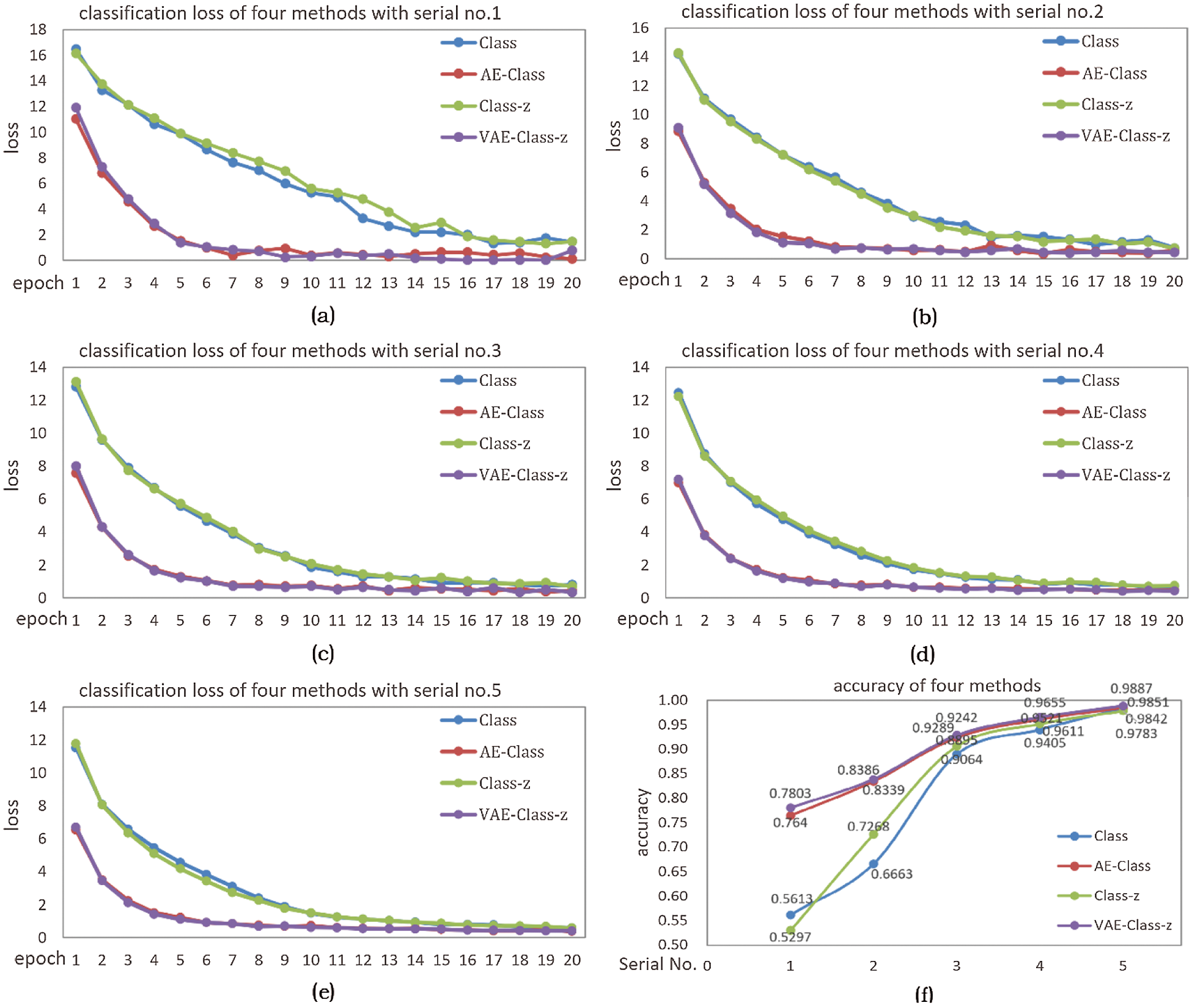
Figure 13: (a)-(e) classification loss corresponding to 5 samples, (f) classification accuracy of the four methods in 5 samples
3.4 Analysis of Detection Results
After expansion, 558 disease images and 463 healthy images are obtained and divided into training set and test set according to the proportion of 7:3. 167 diseased leaf images and 139 healthy leaf images are detected using the Mask R-CNN framework. A total of 818 tomato leaves are detected in 306 images totally, including 240 diseased leaves and 578 healthy leaves. There are 14 identification errors in 240 diseased leaves, and the error identification rate is 5.83%. Only one leaf is identified as healthy leaf, and another 13 diseased leaves are identified as other diseases. Only 0.42% of the diseases are misidentified as healthy leaves, 5.42% of the diseases are mistakenly identified as other diseases. Among 578 healthy leaves, 10 are identified as diseased leaves with an error rate of 1.73%. In conclusion, the correct identification rate of diseased leaves is 94.17%, and only 0.42% of diseased leaves are incorrectly identified as healthy leaves. The correct identification rate of healthy leaves is 98.27%, and only 1.73% of healthy leaves are misidentified as diseased leaves.
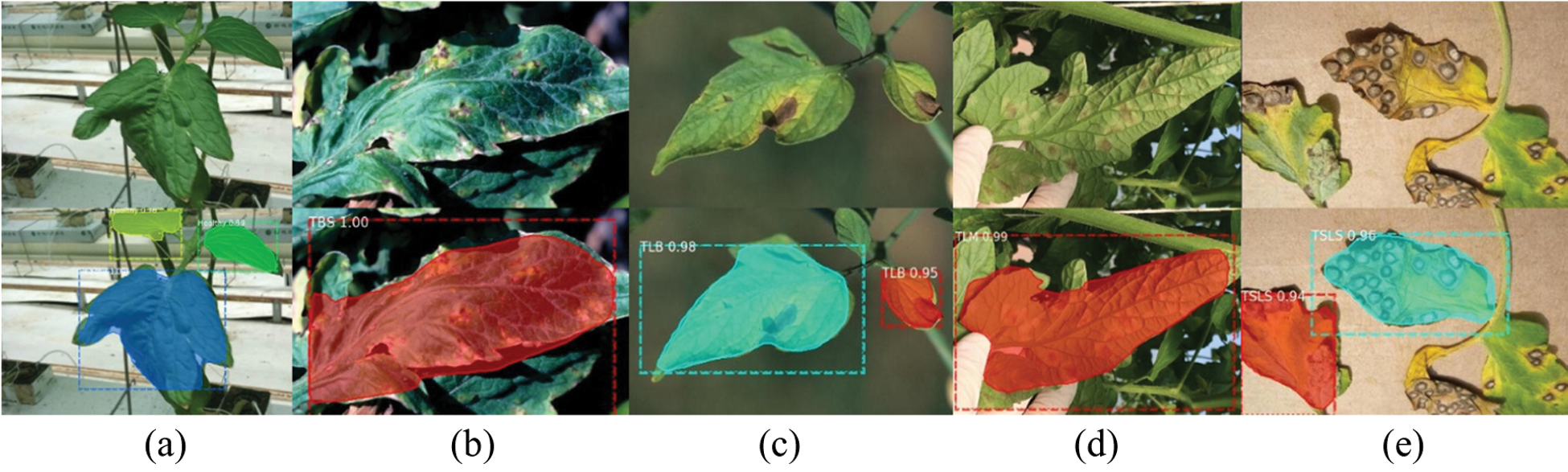
Figure 14: Example of correct detection and identification
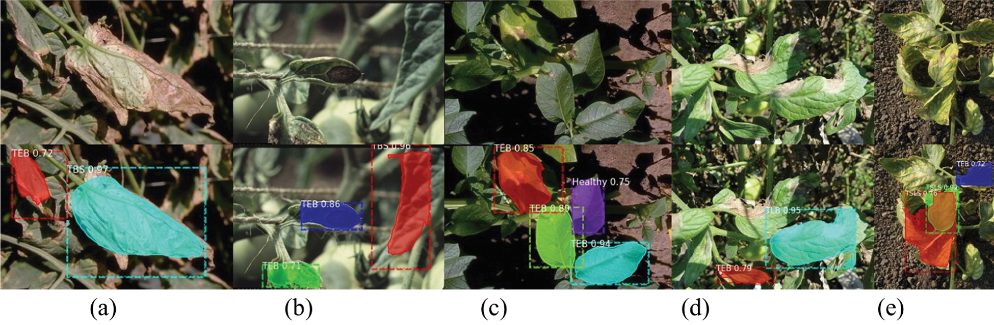
Figure 15: Example of incorrect detection and identification
Figs. 14 and 15 show the correct and incorrect results of detection. The first line in the figure is the original image, and the second line is the detection result. The diseases in the figures are indicated by abbreviations. The actual categories of (a)-(e) in Fig. 15 are TBS, TEB, TEB, TLB, TSLS leaves, respectively. But the identification results are TEB, TBS, healthy, TEB, TEB leaves respectively. The number after the disease category is the confidence of the detection category. For example, “TEB 0.72” means that the confidence of TEB is 0.72.
We find that the dataset is large, but the amount of annotation is relatively small, and thus how to use these unlabeled disease data is a question worth of research. To this end, we propose a lightweight tomato leaf disease identification network supported by VAE enhancement method to improve the identification and detection accuracy of crop leaf diseases. Multi-scale convolution is used to expand the width of the network to make the extracted features more abundant, and deep separable convolution is used to reduce the model parameters, and the lightweight model is applied to the identification network and detection network. We hope our study can be extended to similar application scenarios for crop disease identification.
In the case of fewer labeled samples, the identification accuracy is improved from 56.13% to 78.03%, in the case of more labeled, the identification accuracy has also been improved. The detection results show that the correct identification rate of the disease species is 94.17%, and only 0.42% of the diseased leaves are misidentified as healthy leaves. The correct identification rate of healthy leaves is 98.27%, and only 1.73% of healthy leaves are misidentified as diseased leaves. According to the analysis, the subsequent detection errors can be screened through the confidence threshold and the proportion of the error leaves, thereby further increasing the accuracy of disease identification. The results also show that VAE can enhance the identification and detection of tomato leaf diseases based on proposed lightweight network by making full use of the unlabeled data to overcome the difficulty of labeling. In the future, we will continue to collect more sample images of crop diseases, and use deep convolutional neural network to develop a complete crop disease identification system for agricultural.
Funding Statement: This research was funded by National Natural Science Foundation of China (No. 61973337), Shanghai Municipal Science and Technology Commission Innovation Action Plan of China (No. 17391900900), US National Science Foundation’s BEACON Center for the Study of Evolution in Action (DBI-0939454).
Conflicts of Interest: The authors declare that they have no conflicts of interest to report regarding the present study.
1. H. A. Hiary, S. B. Ahmad, M. Reyalat, M. Braik and Z. Alrahamneh. (2011). “Fast and accurate detection and classification of plant diseases,” International Journal of Computer Applications, vol. 17, no. 1, pp. 31–38. [Google Scholar]
2. C. Song, X. Cheng, Y. Gu, B. Chen and Z. Fu. (2020). “A review of object detectors in deep learning,” Journal on Artificial Intelligence, vol. 2, no. 2, pp. 59–77. [Google Scholar]
3. H. Wu, Q. Liu and X. Liu. (2019). “A review on deep learning approaches to image classification and object segmentation,” Computers, Materials & Continua, vol. 60, no. 2, pp. 575–597. [Google Scholar]
4. B. Hu and J. Wang. (2020). “Deep learning for distinguishing computer generated images and natural images: A survey,” Journal of Information Hiding and Privacy Protection, vol. 2, no. 2, pp. 95–105. [Google Scholar]
5. K. Chen, H. Zhu, L. Yan and J. Wang. (2020). “A survey on adversarial examples in deep learning,” Journal on Big Data, vol. 2, no. 2, pp. 71–84. [Google Scholar]
6. T. Xia, Y. Sun, X. Zhao, W. Song and Y. Guo. (2019). “Generating questions based on semi-automated and end-to-end neural network,” Computers, Materials & Continua, vol. 61, no. 2, pp. 617–628. [Google Scholar]
7. T. Palanisamy, G. Sadayan and N. Pathinetampadiyan. (2019). “Neural network-based leaf classification using machine learning, Concurrency and Computation,” Practice and Experience, vol. 15, pp. e5366. [Google Scholar]
8. P. Zhang and L. Xu. (2018). “Unsupervised segmentation of greenhouse plant images based on statistical method,” Scientific Reports, vol. 8, no. 1, pp. 27. [Google Scholar]
9. Q. Cao and L. Xu. (2019). “Unsupervised greenhouse tomato plant segmentation based on self-adaptive iterative latent dirichlet allocation from surveillance camera,” Agronomy, vol. 9, no. 2, pp. 91. [Google Scholar]
10. M. Brahimi, K. Boukhalfa and A. Moussaoui. (2017). “Deep learning for tomato diseases: Classification and symptoms visualization,” Applied Artificial Intelligence, vol. 31, no. 4, pp. 299–315. [Google Scholar]
11. A. Krizhevsky, I. Sutskever and G. E. Hinton. (2012). “Imagenet classification with deep convolutional neural networks,” in Proc. NIPS. Curran Associates Inc, pp. 1097–1105, . https://dl.acm.org/doi/10.5555/2999134.2999257. [Google Scholar]
12. Y. Wu and L. Xu. (2019). “Crop organ segmentation and disease identification based on weakly supervised deep neural network,” Agronomy, vol. 9, no. 11, pp. 737. [Google Scholar]
13. A. Khamparia, G. Saini, D. Gupta, A. Khanna, S. Tiwari et al. (2020). , “Seasonal crops disease prediction and classification using deep convolutional encoder network,” Circuits, Systems, and Signal Processing, vol. 39, no. 2, pp. 818–836. [Google Scholar]
14. X. Sun, S. Mu, Y. Xu, Z. Cao and T. Su. (2019). “Image recognition of tea leaf diseases based on convolutional neural network. arXiv:1901.02694. [Google Scholar]
15. D. Hughes and M. Salathé. (2015). “An open access repository of images on plant health to enable the development of mobile disease diagnostics,” arXiv:1511.08060. [Google Scholar]
16. K. Simonyan and A. Zisserman. (2014). “Very deep convolutional networks for large-scale image recognition,” arXiv:1409.1556. [Google Scholar]
17. K. He, X. Zhang, S. Ren and J. Sun. (2016). “Deep residual learning for image recognition,” in Proc. CVPR, Las Vegas, NV, USA: IEEE, pp. 770–778. [Google Scholar]
18. C. Szegedy, W. Liu, Y. Jia, P. Sermanet, S. Reed et al. (2015). , “Going deeper with convolutions,” in Proc. CVPR, Boston, MA, USA: IEEE, pp. 1–9. [Google Scholar]
19. C. Szegedy, V. Vanhoucke, S. Ioffe, J. Shlens and Z. Wojna. (2016). “Rethinking the inception architecture for computer vision,” in Proc. CVPR, pp. 2818–2826, . https://ieeexplore.ieee.org/document/7780677. [Google Scholar]
20. T. Michael, A. Jose, U. Thomas, D. Rupesh and H. Sepp. (2016). “Speeding up semantic segmentation for autonomous driving,” in Proc. MLITS, NIPS Workshop, Barcelona, pp. 1–5. [Google Scholar]
21. G. E. Hinton, N. Srivastava, A. Krizhevsky, I. Sutskever and R. Salakhutdinov. (2012). “Improving neural networks by preventing co-adaptation of feature detectors,” Computer Science, vol. 3, no. 4, pp. 212–223. [Google Scholar]
22. A. G. Howard, M. Zhu, B. Chen, D. Kalenichenko and W. Wang. (2017). “Mobilenets: Efficient convolutional neural networks for mobile vision applications,” arXiv:1704.04861. [Google Scholar]
23. X. Zhang, X. Zhou, M. Li and J. Sun. (2018). “Shufflenet: An extremely efficient convolutional neural network for mobile devices,” in Proc. CVPR, pp. 6848–6856, . https://ieeexplore.ieee.org/document/8578814. [Google Scholar]
24. D. P. Kingma and M. Welling. (2013). “Auto-encoding variational bayes,” arXiv:1312.6114. [Google Scholar]
25. S. Ren, K. He, R. Girshick and J. Sun. (2017). “Faster R-CNN: Towards real-time object detection with region proposal networks,” IEEE Transactions on Pattern Analysis and Machine Intelligence, vol. 39, no. 6, pp. 1137–1149. [Google Scholar]
26. K. He, G. Gkioxari, P. Dollar and R. Girshick. (2020). “Mask R-CNN,” IEEE Transactions on Pattern Analysis and Machine Intelligence, vol. 42, no. 2, pp. 386–397. [Google Scholar]
27. S. Christian, I. Sergey, V. Vincent and A. Alex. (2017). “Inception-v4, inception-resnet and the impact of residual connections on learning,” in Proc. AAAI, . https://dl.acm.org/doi/10.5555/3298023.3298188. [Google Scholar]
28. M. Sandler, A. Howard, M. Zhu, A. Zhmoginov and L. Chen. (2018). “Mobilenetv2: Inverted residuals and linear bottlenecks,” in Proc. CVPR, pp. 4510–4520, . https://ieeexplore.ieee.org/document/8578572. [Google Scholar]
 | This work is licensed under a Creative Commons Attribution 4.0 International License, which permits unrestricted use, distribution, and reproduction in any medium, provided the original work is properly cited. |