DOI:10.32604/iasc.2021.016802
| Intelligent Automation & Soft Computing DOI:10.32604/iasc.2021.016802 | |
| Article |
A Fog Covered Object Recognition Algorithm Based On Space And Frequency Network
1College of Equipment Management and Support, Engineering University of PAP, Xi’an, 710086, China
2Key Laboratory of Spectral Imaging Technology CAS, Xi’an Institute of Optics and Precision Mechanics, Chinese Academy of Sciences, Xi’an, 710119, China
3University of California, Los Angeles, California, 90095, USA
*Corresponding Author: Shi Qiu. Email: qiushi215@163.com
Received: 12 January 2021; Accepted: 19 February 2021
Abstract: It is difficult to recognize a target object from foggy images. Aiming at solving this problem, a new algorithm is thereby proposed. Fog concentration estimation is the prerequisite for image defogging. Due to the uncertainty of fog distribution, a fog concentration estimation model is accordingly proposed. Establish the brightness and gradient model in the spatial domain, and establish the FFT model in the frequency domain. Also, a multiple branch network framework is established to realize the qualitative estimation of the fog concentration in images based on comprehensive analysis from spatial and frequency domain levels. In the aspect of foggy image target recognition, a residual network is introduced based on Fast RCNN network structure. The fog concentration information is added into the target recognition function to realize accurate recognition of target from foggy images. Experimental results show that the accuracy of AOM is higher than 81 under different fog concentration indoors and outdoors.
Keywords: Foggy image; fog concentration; estimation; target object recognition; fog removal; deep learning
Fog is an aerosol system composed of a large number of tiny water droplets or ice crystals suspended in the air near the ground, which can cause blurred vision and low visibility [1–3]. Therefore, fog removal in images is a focus and hot issue of current research. He et al. [1] proposes an image defogging algorithm based on dark channel, and it yields good results. Matlin et al. [4] establishes a model to remove fog and noise from a single image. Ullah et al. [5] improves the dark channel operator to realize fast defogging. Zhang et al. [6] establishes a model for night fog distribution. Li et al. [7] removes fog according to boundary features. Yang et al. [8] uses a method of super-pixel to realize defogging. Ju et al. [9] improves an atmospheric scattering model to remove fog. Xie et al. [10] establishes a model for adaptive defogging according to the characteristics of remote sensing images. Shafina et al. [11] improves the airtight estimation by gradient threshold to remove fog in a single image. Mittal et al. [12] uses multiple thresholds to remove fog. Liu et al. [13] uses gray histogram to detect fog area. Fog concentration estimation is the prerequisite for image defogging.
In recent years, scholars have studied fog weather phenomenon recognition from different perspectives and achieved some results. Heinle et al. [14] automatically distinguishes sunny days from other weather in sky images. Yu et al. [15] establishes an SVM model to determine whether the image contains fog. Kong et al. [16] distinguishes fog area from spectral reflection and absorption. Liu et al. [17] uses the gray histogram to detect fog area. Pavlic et al. [18] obtains images from driving perspective to distinguish foggy and non-foggy areas. Zhang et al. [19] extracts image features and classifies fog images. Makarau et al. [20] establishes an empirical and automatic method to realize fog detection. Zhang et al. [21] extracts multiple weather features and takes proper processing. Thakur et al. [22] judges the concentration of fog from the perspective of image blur. Zhang et al. [23] establishes multiple learning systems to check the classification of multiple weather. Wan et al. [24] establishes a GMM model and divides images into 3 model: no fog, mist and thick fog. Wang et al. [25] integrates real-time weather information into the image. Chen et al. [26] combines multiple features to judge weather conditions comprehensively.
2 Fog Concentration Estimation Algorithm
According to the characteristics of fog imaging, we establish a brightness and gradient model in the spatial domain and an energy model in the frequency domain to comprehensively estimate the fog density, build a deep learning framework, and achieve target recognition. Then fog concentration can be comprehensively estimated. Finally, a deep learning framework is constructed to realize target object recognition, as shown in Fig. 1.

Figure 1: Flow chart of the proposed algorithm
2.1 Space and Frequency Fusion Model
Fog will cause the image to be blurred, the mist image is displayed as a hazy and light-toned image, and the thick fog image is displayed as the image is white and attached to the surface of the scene. Therefore, the image brightness information is an effective information for estimating the fog density. The image texture reflects the gray level repetition or changes between image pixels. As the fog density increases, the image texture information will gradually become blurred. Therefore, the image texture information is an effective information for estimating the fog density.
The denser the fog in the area, the more serious the reflection of the object will be affected by the suspended particles, and the greater the proportion of full light in imaging, resulting in the area with high brightness and blurred texture. The fog density is proportional to the brightness characteristics and the texture characteristics. Inversely. Thus, a model is constructed:
where L is the brightness feature distribution, P is the texture feature distribution, and α is the weight factor.
where Ω(bi) refers to the neighborhood centered on bi, and B represents the number of pixels in the neighborhood, I and ▽I are the normalized brightness map and gradient map, respectively.
Due to the unavoidable texture noise interference, the discontinuity of D in the approximate depth area is caused, and the fog density is basically constant when the scene depth is the same, so D cannot directly reflect the real fog density distribution. Therefore, it is necessary to remove the texture details as much as possible on the premise of retaining its original depth information. Due to the edge and noise rejection of the guided filter, the filter is constructed:
where
Since the spatial image is intertwined with targets, background, noise, and fog, the analysis of the spatial image cannot fully display the fog information. For this reason, this section builds a model from the energy point of view to realize fog density estimation. When the image contains more detailed information, the greater the energy, and vice versa. That is, the larger the value of the atmospheric light transfer function, the lower the fog density and the higher the spectrum energy.
where the image resolution is M×N, F(u,v) is the Fourier transform of I(x,y).
The frequency domain model represents the energy distribution in the area, and the pixel value of a single point cannot reflect the distribution of fog. Therefore, the image is divided into blocks with the resolution of m×m, and the image energy distribution map is obtained.
2.2 Fog Concentration Estimation Network
After extracting the features, it is necessary to make full use of the features to classify the foggy images. With the rise of neural networks, deep learning is increasingly applied to classification problems. Deep learning is to superimpose nonlinear layers, so that deep neural networks can fit complex nonlinear mapping. Due to the gradual superposition of the number of network layers, the problems of network convergence and optimization difficulties arise. To this end, ResNet [27,28] is introduced, and its main idea is to add cross-layer connections in different convolutional layers and change the mapping relationship between layers. The network structure is shown in Fig. 2.

Figure 2: Network structure of fog concentration estimation
With ResNet structure, the nonlinear mapping actually learned by the network is F(X) = H(X)-X. Overlaying the number of layers of convolutional neural networks will make the model more complex. The deeper neural networks theoretically show better generalization performance, but the results show that when the network depth reaches a certain number of layers, the error on the training set began to increase gradually. Increasing cross-layer connections and reducing network optimization make it easier for deep networks to achieve convergence. ResNet compromises complex networks and simple networks to adapt to classification modes of varying complexity.
Three residual blocks with the same number of feature images are used as a scale, and three scales with the number of feature maps are used to form the feature extraction part in the residual network, and the maximum pooling between each scale is used to reduce the number of feature map pixels. When the number of F(X) and X feature maps is inconsistent, a 1×1 convolution kernel is used for transformation. This paper constructs a three-branch network, and each branch network shares the shallow feature extraction in scale1 and scale 2. ResNet1, 2, 3 use independent cross entropy loss functions, and different scales are set in scale 3.
In the convolution kernel, the gradient between scale1 and scale 2 is a regular relationship, and the weight of a convolution layer in scale 2 is Wc, and the corresponding gradient is as follows:
where Rn represents the loss function of ResNet n. Different sizes of convolution kernels have different receptive fields. The interface between scale and scale 3 input part convolution layer, the partial derivative of the loss function to the activation value of its characteristic graph is:
where H and W are the height and width of the output convolution feature graph. ahw is the activation value of the output convolution feature graph. dZhwc is a loss function with respect to the pixel value of the feature image before the output convolution layer (h, w, c) is activated. The weight update gradients in scale 1 and scale 2 are returned by dA. Finally, the network generates mixed adjustment of multiple gradients in the shared weight part, in order to improve the generalization performance of single branch network.
Network training can be regarded as the fusion of sub networks according to specific rules, in which the regularization method can randomly train the network after a certain proportion of inactivated neurons. This paper uses regularization to further improve the generalization performance of the model, and obtain the probability q1 that the pixel is foggy, The probability of no fog q2, (q1 + q2 = 1) We further enhance the data: fill the edges of the original image, randomly crop the image with a size of 32 × 32 × 3, and randomly change the brightness, contrast, and flip to enhance Model training data.
2.3 Target Object Recognition Model
Fast RCNN is a mainstream method for target object recognition [29]. The whole object candidate area, depth feature and object recognition are integrated into a depth network, and the loss function is as follows:
where pi is the probability that the i-th candidate box is a positive sample; ti and
Since the target is contained in the fog, and the fog is not evenly distributed in the image, the strength of the fog density will directly affect the effect of target recognition. Through the research in the previous section, we have obtained the estimated probability of the fog concentration, we introduce it into the above formula, and the revised objective function is:
In order to improve the algorithm recognition effect, the method of increasing the number of network layers is often used. However, the ever-increasing network depth will make the back propagation gradient unstable, leading to increased training errors. The residual network superimposes the input and output to improve the model recognition effect. The output of the two-layer residual module can be expressed as:
where σ is the activation function, W1 and W2 are the network weights; Ws is the input weight, so as to achieve accurate target object recognition. The network structure is shown in Fig. 3.

Figure 3: RESNET cross layer connection diagram
3 Experiment and Result Analysis
In the experiment, images of different fog density taken by a fixed camera were used to form a data group, a total of 5000 frames of images, and the fog density was manually sorted as the gold standard.
Sensitivity (SEN): Reflects the detection performance of the algorithm on real targets. Specificity (SPE): Reflects the detection performance of the algorithm on false targets. Accuracy (ACC): Reflects the ratio of correct test results to all samples in test results. False Positive Fraction (FPF): Reflects the ratio of false positives that are diagnosed as true targets [30,31].
where TP is True Positive, TN is True Negative, FP is False Positive, FN is False Negative.
Area overlap measure (AOM) is defined as the evaluation index of segmentation effect.
where, AOM is the area overlap degree, A is the marked image, and B is the recognition result map, which indicates the number of pixels in the corresponding area. The larger the AOM value, the better the segmentation effect.
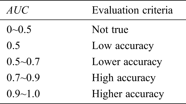
The ROC curve is an objective criterion for evaluating the performance of two or more image classification algorithms. The area under the ROC curve (AUC) can be used as a reference standard for measuring the accuracy of diagnosis and classification [32]. The evaluation results are as Tab. 1.
Table 1: AUC evaluation criteria
DATA1: Mark the foggy and non-fog images of the fixed camera, and group the foggy and non-fog images of the same target at the same time period into 1 group (total 1000 groups), and then compare the classification effects of different algorithms.
From Tab. 2 and Fig. 4, in this paper, it can be seen that the spatial and frequency domain algorithms proposed in this paper achieve the classification of foggy and non-fog images to a certain extent, but they are not as effective as the Ambiguity model [22] and the GMM model [24]. The Ambiguity model [22] establishes a model to achieve classification according to the degree of blurring of the spatial image. The GMM model [24] algorithm predicts the distribution of image fog from the perspective of probability analysis to achieve image classification. In this paper, the spatial and frequency domain models are established from the perspective of boundary and energy, and the above two models are merged to realize the classification of foggy and non-fog images, and good results have been achieved.
Table 2: The effect of fog image classification

DATA2: Mark the foggy and non-fog images of the fixed camera. DATA2 is more difficult than DATA1. It can be seen from Tab. 3 and Fig. 5 that the performance of all algorithms has decreased, but the algorithm proposed in this paper constructs models from two levels: space domain and frequency domain. Analyze the fog distribution from a macro perspective to realize image classification. The algorithm performance is still the best compared with other algorithms.
Table 3: The effect of fog image classification

Mark the foggy and non-fog images of the fixed camera, form a group of images with different fog density taken on the same target at the same time period, input 2 frames of pictures into the system, perform a 2-classification algorithm to select the foggy image, and then iterate get the fog density ranking image. And artificially sort the fog density by size from a visual angle. When the graph group 6 is input as Fig. 6, the algorithm sorting result is 123, which is consistent with the manually labeled one. When the graph group 6 is input as Fig. 7, the sorting result of the algorithm is 12435, which is inconsistent with the manual sorting. The reason is that the fog distribution in Fig. 7-4 is more even than that in Fig. 7-3, and the calculation value of the algorithm is higher locally, leading to analysis errors. But overall the sorting accuracy rate reached 98%, which greatly improved work efficiency.
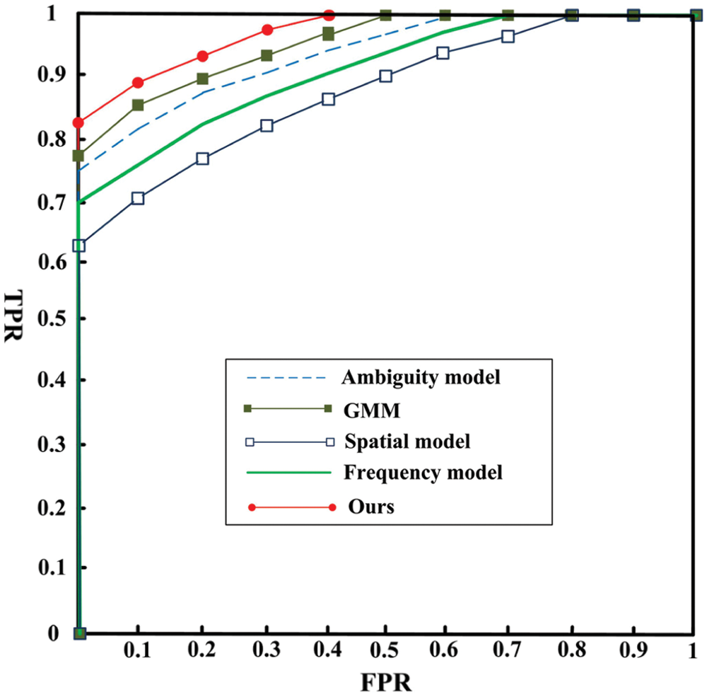
Figure 4: ROC curves of DATA1 fog classification algorithms

Figure 5: ROC curves of DATA2 fog classification algorithms

Figure 6: Fog concentration order images

Figure 7: Fog concentration order images
All images are taken by same camera both indoors and outdoors to carry out the experiment. The results marked by professionals are the gold standard. Target object recognition effect shown as in Tab. 4. It can be seen that the algorithm proposed in this paper has achieved good results in indoor and outdoor images with different fog concentrations, and the AOM is above 0.81. Theeffect images of target object recognition in foggy images shown as in Fig. 8.
Table 4: Object recognition effect


Figure 8: The effect images of object recognition in fog images
The effect comparison of target object recognition under mist and thick fog condition: The target recognition effect of mist is better than that of thick fog. This is because the haze has less influence on the target, and the characteristics of the target are more obvious. It can better distinguish the difference between the target and the background. With the increase of fog density, the characteristics of the target are gradually submerged into the fog. Through the fog density estimation model and target recognition network proposed in this paper, part of the target characteristics can be restored. However, when the fog density is too thick, the algorithm has limited recovery characteristics, resulting in a decrease in the effect.
The effect comparison of indoors and outdoors: The indoor target recognition effect is better than the outdoor target recognition effect. This is because the indoor scene light is relatively soft, and mostly close-up images, the camera obtains the target information more accurately. Outdoor scenes have weaker light and more complex backgrounds, and are mostly distant images. The camera’s acquisition of target information is blurry. The effect of the algorithm has decreased.
Aiming at the problem of difficult identification of foggy image targets, this article proposes a model based on the spatial and frequency domain feature fusion, and builds a deep learning network to estimate the fog density. Then the fog density information is fused to the target recognition network, the residual network is introduced, and the target function is modified to achieve accurate target recognition. However, there are still some problems with the problem of excessive fog density and blurred target characteristics caused by blurred distant images, therefore further research is needed.
Acknowledgement: This work is supported by Postdoctoral Science Foundation of China under Grant No. 2020M682144. Basic research project of engineering university of PAP under Grant No. WJY202145. The Open Project Program of the State Key Lab of CAD&CG under Grant No. A2026, Zhejiang University.
Funding Statement: The author received no specific funding for this study.
Conflicts of Interest: The authors declare that they have no conflicts of interest to report regarding the present study.
1. K. He, J. Sun and X. Tang. (2011). “Single image haze removal using dark channel prior,” IEEE Transactions on Pattern Analysis and Machine Intelligence, vol. 33, no. 12, pp. 2341–2353. [Google Scholar]
2. M. B. Nejad and M. E. Shir. (2019). “A new enhanced learning approach to automatic image classification based on SALP swarm algorithm,” Computer Systems Science and Engineering, vol. 34, no. 2, pp. 91–100. [Google Scholar]
3. N. Mohanapriya and B. Kalaavathi. (2019). “Adaptive image enhancement using hybrid particle swarm optimization and watershed segmentation,” Intelligent Automation and Soft Computing, vol. 25, no. 4, pp. 663–672. [Google Scholar]
4. E. Matlin and P. Milanfar. (2012). “Removal of haze and noise from a single image, Computational Imaging X,” International Society for Optics and Photonics, vol. 8296, pp. 82960T. [Google Scholar]
5. E. Ullah, R. Nawaz and J. Iqbal. (2013). “Single image haze removal using improved dark channel prior,” in 2013 5th Int. Conf. on Modelling Identification and Control (ICMICCairo, Egypt: IEEE, pp. 245–248. [Google Scholar]
6. J. Zhang, Y. Cao and Z. Wang. (2014). “Nighttime haze removal based on a new imaging model,” in IEEE Int. Conf. on Image Processing (ICIPParis, France: IEEE, pp. 4557–4561. [Google Scholar]
7. Z. Li and J. Zheng. (2015). “Edge-preserving decomposition-based single image haze removal,” IEEE Transactions on Image Processing, vol. 24, no. 12, pp. 5432–5441. [Google Scholar]
8. M. Yang, Z. Li and J. Liu. (2016). “Super-pixel based single image haze removal,” in 2016 Chinese Control and Decision Conf. (CCDCYinchuan, China: IEEE, pp. 1965–1969. [Google Scholar]
9. M. Ju, Z. Gu and D. Zhang. (2017). “Single image haze removal based on the improved atmospheric scattering model,” Neurocomputing, vol. 260, no. 6, pp. 180–191. [Google Scholar]
10. F. Xie, J. Chen, X. Pan and Z. Jiang. (2018). “Adaptive haze removal for single remote sensing image,” IEEE Access, vol. 6, pp. 67982–67991. [Google Scholar]
11. M. Shafina and S. Aji. (2019). “A single image haze removal method with improved airlight estimation using gradient thresholding,” Integrated Intelligent Computing, Communication and Security. Singapore: Springer, pp. 651–659. [Google Scholar]
12. M. Mittal, M. Kumar, A. Verma, I. Kaur, B. Kaur et al. (2021). , “FEMT: A computational approach for fog elimination using multiple thresholds,” Multimedia Tools and Applications, vol. 80, no. 1, pp. 227–241. [Google Scholar]
13. W. Liu, X. Hou, J. Duan and G. Qiu. (2020). “End-to-end single image fog removal using enhanced cycle consistent adversarial networks,” IEEE Transactions on Image Processing, vol. 29, pp. 7819–7833. [Google Scholar]
14. A. Heinle, A. Macke and A. Srivastav. (2010). “Automatic cloud classification of whole sky images,” Atmospheric Measurement Techniques, vol. 3, no. 3, pp. 557–567. [Google Scholar]
15. X. Yu, C. Xiao, M. Deng and L. Peng. (2011). “A classification algorithm to distinguish image as haze or non-haze,” in Sixth Int. Conf. on Image and Graphics, Hefei, China: IEEE, pp. 286–289. [Google Scholar]
16. X. Kong, Y. Qian and A. Zhang. (2011). “Haze and cloud cover recognition and removal for serial Landsat images, MIPPR 2011: Remote Sensing Image Processing, Geographic Information Systems, and Other Applications,” International Society for Optics and Photonics, vol. 8006, pp. 80061K. [Google Scholar]
17. Y. Liu and X. Lu. (2012). “Fog detection and classification using gray histograms,” Advanced Materials Research. Trans Tech Publications, vol. 403, pp. 570–576. [Google Scholar]
18. M. Pavlic, G. Rigoll and S. Ilic. (2013). “Classification of images in fog and fog-free scenes for use in vehicles,” in 2013 IEEE Intelligent Vehicles Sym. (IVGold Coast, QLD, Australia: IEEE, pp. 481–486. [Google Scholar]
19. Y. Zhang, G. Sun, Q. Ren and D. Zhao. (2013). “Foggy images classification based on features extraction and SVM,” in 2013 Int. Conf. on Software Engineering and Computer Science, Atlantis Press. [Google Scholar]
20. A. Makarau, R. Richter, R. Müller and P. Reinartz. (2014). “Haze detection and removal in remotely sensed multispectral imagery,” IEEE Transactions on Geoscience and Remote Sensing, vol. 52, no. 9, pp. 5895–5905. [Google Scholar]
21. Z. Zhang and H. Ma. (2015). “Multi-class weather classification on single images,” in 2015 IEEE Int. Conf. on Image Processing (ICIPQuebec City, QC, Canada: IEEE, pp. 4396–4400. [Google Scholar]
22. R. Thakur and C. Saravanan. (2016). “Classification of color hazy images,” in Int. Conf. on Electrical, Electronics, and Optimization Techniques (ICEEOTChennai, India: IEEE, pp. 2159–2163. [Google Scholar]
23. Z. Zhang, H. Ma, H. Fu and C. Zhang. (2016). “Scene-free multi-class weather classification on single images,” Neurocomputing, vol. 207, pp. 36. [Google Scholar]
24. J. Wan, Z. Qiu, H. Gao, F. Jie and Q. Peng. (2017). “Classification of fog situations based on Gaussian mixture model,” 36th Chinese Control Conf. (CCC), Dalian: IEEE, pp. 10902–10906. [Google Scholar]
25. S. Wang, Y. Li and W. Liu. (2018). “Multi-class weather classification fusing weather dataset and image features,” CCF Conf. on Big Data, Singapore: Springer, pp. 149–159. [Google Scholar]
26. Y. Chen, J. Wang, S. Li and W. Wang. (2019). “Multi-feature based foggy image classification,” IOP Conference Series: Earth and Environmental Science. IOP Publishing, vol. 234, no. 1, pp. 012089. [Google Scholar]
27. Z. Wu, C. Shen and D. Van. (2019). “Wider or deeper: Revisiting the resnet model for visual recognition,” Pattern Recognition, vol. 90, no. 3, pp. 119–133. [Google Scholar]
28. S. Niu, X. Li, M. Wang and Y. Li. (2020). “A modified method for scene text detection by resnet,” Computers, Materials & Continua, vol. 65, no. 3, pp. 2233–2245. [Google Scholar]
29. X. Hong, X. Zheng, J. Xia and W. Xue. (2019). “Cross-lingual non-ferrous metals related news recognition method based on cnn with a limited bi-lingual dictionary,” Computers, Materials & Continua, vol. 58, no. 2, pp. 379–389. [Google Scholar]
30. S. Qiu, J. Luo, S. Yang, M. Zhang and W. Zhang. (2019). “A moving target extraction algorithm based on the fusion of infrared and visible images,” Infrared Physics & Technology, vol. 98, no. 1, pp. 285–291. [Google Scholar]
31. Z. Huang, Y. Fu and F. Dai. (2017). “Study for Multi-resources spatial data fusion methods in big data environment,” Intelligent Automation & Soft Computing, vol. 24, no. 1, pp. 1–6. [Google Scholar]
32. Partial-Duplicate. (2020). “Image search,” ACM Transactions on Multimedia Computing, Communications, and Applications, vol. 16, no. 2, pp. 1–25. [Google Scholar]
 | This work is licensed under a Creative Commons Attribution 4.0 International License, which permits unrestricted use, distribution, and reproduction in any medium, provided the original work is properly cited. |