DOI:10.32604/iasc.2021.016272
| Intelligent Automation & Soft Computing DOI:10.32604/iasc.2021.016272 | |
| Article |
Driving Pattern Profiling and Classification Using Deep Learning
1Department of Computer Science and Engineering, U.I.E.T, Maharshi Dayanand University, Rohtak, 124001, India
2Department of Computer Science and Engineering, SRM University, Delhi-NCR, Sonipat, 131029, India
3Department of Computer Science and Engineering, Graphic Era Hill University, Uttarakhand, 248171, India
4Institute of Research and Development, Duy Tan University, Danang, 550000, Vietnam
5Faculty of Information Technology, Duy Tan University, Danang, 550000, Vietnam
*Corresponding Author: Dac-Nhuong Le. Email: ledacnhuong@duytan.edu.vn
Received: 29 December 2020; Accepted: 05 March 2021
Abstract: The last several decades have witnessed an exponential growth in the means of transport globally, shrinking geographical distances and connecting the world. The automotive industry has grown by leaps and bounds, with millions of new vehicles being sold annually, be it for personal commuting or for public or commodity transport. However, millions of motor vehicles on the roads also mean an equal number of drivers with varying levels of skill and adherence to safety regulations. Very little has been done in the way of exploring and profiling driving patterns and vehicular usage using real world data. This paper focuses on extracting and classifying distinct driving patterns using actual, dynamic vehicular data collected from the “On Board Diagnostics” port present (by default) in most vehicles. “Machine learning” and “Deep Learning” techniques were thereafter employed to extract and derive insights from observed patterns in the data. Various algorithms like hierarchical clustering, k-means clustering, multinomial naive bays, artificial neural networks and multi-layer perceptron were used to construct models to extract driving patterns and classify the data and ultimately generate insights about driver behavior across various parameters. The Inter-Class-ReLU was used to generate activation functions for the production of logical neurons and to develop and present a model that can classify incoming data into various groups and precisely identify distinct driving patterns. The developed model can be utilized in public as well as personal vehicles for monitoring driving behavior and driver preferences so that irregular behavior of a certain driver of a particular vehicle for a specified period can be scrutinized with ease.
Keywords: On board diagnostics; hierarchical clustering; k-means clustering; multinomial Naive Bayes; artificial neural networks; multilayer perceptron
With the number of vehicles in our cities multiplying at an alarming rate and a marked increase in road accidents, pollution levels and traffic related woes, the human component (the driver) involved in the process of driving can hardly be ignored. A comprehensive understanding of driving patterns and the impact thereof, can aid in identifying distinct driving behaviors which are likely to undermine the safety of not only the vehicle and its passengers, but also pedestrians and other vehicles on the road. Such an analysis can be instrumental in promoting safety on the roads as well as in identifying fuel-efficient driving and drivers who might benefit from specific training or restraining.
Such a data driven approach can ensure that all transport vehicles, regardless of their type, are utilized up to their regulatory thresholds, especially private vehicles which tend to be used to their maximum potential [1]. Consequently, monitoring of driving behaviors can be made obligatory, in order to promote good behavior and proficient fuel consumption, in keeping with the current green environment norms and initiatives [2,3]. Furthermore, with the advent of driver-less vehicles in the near future, analysis of stored data in automobiles can become a significant factor in continuous monitoring as well as in upcoming audits. Such data can be especially advantageous for establishments that are accountable for transportation substructure planning, discipline and care, for insurance specialists and agencies, as well as for law enforcement agencies [4].
In this research, a model has been developed using data collected from the On-Board Diagnostics (OBD) device which is fitted inside most contemporary vehicles. This device collects instantaneous data from various vehicular components and is used to monitor their operational health. This data was first collected from the OBD device and then cleaned and pre-processed before being fed into the model. The data was then grouped into different clusters using clustering algorithms in order to discover discernible patterns. A thorough analysis of these patterns was then undertaken in order to understand their real-life applications and significance. Subsequently, multiple ML and DL techniques and algorithms were utilized in order to develop a classifier for classifying testing data into different groups. In this paper artificial neural networks were used and a weighted mean precision of about 98.68% was achieved.
Several works of literature have been identified that have sought to analyze driving behavior using various approaches like multi-sensor fusion, image processing, computer vision, etc. In Kishimoto et al. [5] the authors have proposed a model using HMM (Hidden Markov Model) on historic driving data in order to calculate the probability of a driver applying brakes. In Osgouei et al. [6] the writers presented a driving behavior analysis model for multiple drivers that was based on objective principles that were finalized by the HMM model arbitrarily. The authors in Vaitkus et al. [7] proposed a model for the automatic classification of driving styles using pattern recognition which uses data from a 3- axis accelerometer installed in the test vehicle. In Fazeen et al. [8] the authors used a 3-dimensional accelerometer along with an android phone’s GPS or “Global Positioning System”. The phone was used to capture and analyze driver behavior as well as road conditions. In Dai et al. [9] the authors used mobile phones secured in the vehicles for detecting drunken driving patterns. This was undertaken using accelerometers in the mobile phones and by measuring the vehicle’s longitudinal and lateral acceleration and then comparing and correlating these patterns with driving test data. In Othman et al. [10] and Murphey et al. [11] the authors used the first derivative of acceleration (rate of change in acceleration -jerks) to analyze and classify driving styles. In Lotan et al. [12] an In-Vehicle Data Recorder was used by the author to understand the driving moves and to arrange them into various categories, viz., dangerous, unsafe and safe. The paper did not offer any information on the methodology of resolution of the driving patterns; the creators contrasted new age drivers and guardians. In particular, the correlation uncovered contrasts, if any, present in the number of hazardous and unsafe moves on a day-to-day basis. Accident coverage organizations are especially concerned about the safety of drivers, crash potential, crash rates and driving profiles. A few insurance agencies in fact, have recommended that their clients deliberately utilize IVDRs to record their day to day driving [13]. In Zhang et al. [14] the authors proposed an end-to-end deep learning framework using CNN and RNN neural networks by utilizing data captured with an in-vehicle Controller Area Network-BUS (CAN-BUS). In Bernardi et al. [15] the authors projected a bunch of behavioral features mined using a car monitoring system which could culminate in a driver identification system to appraise the driver’s knowledge and know-how regarding a particular vehicle. The proposed feature model was used with a time-series classification approach based on a MLP “multilayer preceptor” on technique. In Choi et al. [16] the authors used HMMs “Hidden Markov Models” to obtain a pattern of driving characteristics gathered from the vehicle’s CAN-Bus (Controller Area Network) information. The paper describes and models driver behavior using the data from parameters like brake status, steering wheel angle, vehicle speed and acceleration status. These models served three different tasks such as action classification, distraction detection, and driver identification. In Miyajima et al. [17] the authors modeled driving behaviors. An on linear function with statistical method of a Gaussian mixture model was utilized to model the connection between vehicle velocity and the subsequent distance which was mapped into a two-dimensional space. GMMs were also used to model pedal operation patterns.
This paper [18] undertook a study with dissimilar sensors of Android smartphone, and classification algorithms so as to evaluate which sensor assembly or technique could allow for classifications with advanced performance. The outcomes demonstrated that smart approaches and exact arrangements of sensors led to enhanced classification performances. Further wide-ranging approaches related to connected and smart communities were perceived and realized in an endeavor by Sun and colleagues [19]. The work by Engel Brecht and colleagues [20] also yielded excellent results during a detailed evaluation of smartphone-based sensing in vehicles.
An OBD-II reader is intended to measure air flow mass and speed from which fuel consumption and distance are also calculated. Afterwards this data is transmitted to a remote server through Wi-Fi. GPS tracking is also tooled by this system so as to determine the location of vehicle. A DMS “database management system” is applied at the remote server for the management and storage of transmitted data and a GUI “Graphical User Interface” is established for transmitted data evaluation. The authors adopted a relaxed method for car data stimulation and also demonstrated the availability of current platforms along with guidance for utilizing the same. The fundamental target of this system was behavior monitoring of the driver during the driving time. Using this the owner can not only monitor the fuel consumption but also the driving pattern and driver behavior. Probability of accidents utilizing ANN “Artificial Neural Network” approaches has also been endeavored. Traffic accident data has been used in this system with the OBD “On Board Diagnostic” as mode testing and training samples. [21–24]. MiJin Kim proposed a system which obeyed standards of OBD II and could observe and administer multiple kinds of vehicle faults and flaws [25]. Participation of large organizations such as owners of transportation fleet, insurance corporations of government, authorities of transport, etc. were made possible by a web interface for the calculation of results of an anticipated set of vehicles or people through an extensive use of big data, block chain technology and analytics [26,27]. Driver monitoring and vehicle diagnostics experiments at the headquarters of Android CarLab were undertaken. OBD-II connectors were implemented and integrated with Wi-Fi, Bluetooth and WCDMA modules for data extraction. An intelligent RDD management technique was utilized so that capability and efficiency of the spark could be increased. CNN “Convolution neural network” based techniques studied the traffic as digital images and forecast large-scale, network-wide traffic speed with great accuracy, with an accuracy of 42.91% within a satisfactory performance time limit [28–31].
In this research, unsupervised machine learning algorithms were used to extract driving patterns from the data which was collected using the On-Board Diagnostics (OBD) device of a car. The OBD or On-Board Diagnostics was originally developed and designed to continuously monitor the major components of the engine of a vehicle. It is a self-diagnostic device of the vehicle. It adopts a uniform technique for diagnostic trouble codes, accessing data and a lot of additional information from different types of vehicles including cars as well as medium and heavy-duty vehicles. The original purpose of using OBD was to obtain live data in addition to standardized diagnostic trouble codes which could assist repair technicians in identifying and fixing glitches within the vehicle. It was initially introduced for the purposes of monitoring the function of emission control components of a vehicle. The OBD II, which is the next generation of the original OBD, comes with an even wider range of diagnostics. In this research, an external hardware compatible with the OBD-II port was used for data collection. The data was collected and stored on an SD card attached to the external board. Fig. 1 shows the methodology used in this research in a flowchart pattern.

Figure 1: The methodology
Data pre-processing is a vital step in the development of a machine learning model, where data is encoded and transformed to a machine-level language, enabling a machine to easily parse it. The data which is obtained from the OBD of the vehicle consists of multiple parameters. The values of these parameters are used to interpret the instantaneous performance of the different components of the engine. The emphasis of the paper is to derive and uncover dissimilar driving patterns through data of underlying features that are directly prejudiced by the driving style of the driver. These include parameters like engine power, engine rpm, load on engine, vehicle speed, position of throttle and coolant temperature.
Fig. 2 shows the OBD port in the car which was used to collect the data and Fig. 3 illustrates the different pins and their positions in the OBD port. Figs. 4 to 7 demonstrate the distribution of data points in the dataset chosen for this study, with speed on the y-axis and features like engine RPM, engine load, throttle position, and coolant temperature on the x-axis. Fig. 8 demonstrates how the engine load varies with the throttle position in the dataset.
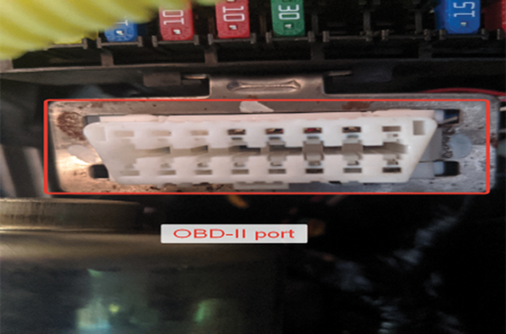
Figure 2: OBD-II port in car

Figure 3: Pins in OBD-II port

Figure 4: Instantaneous speed vs. instantaneous engine RPM
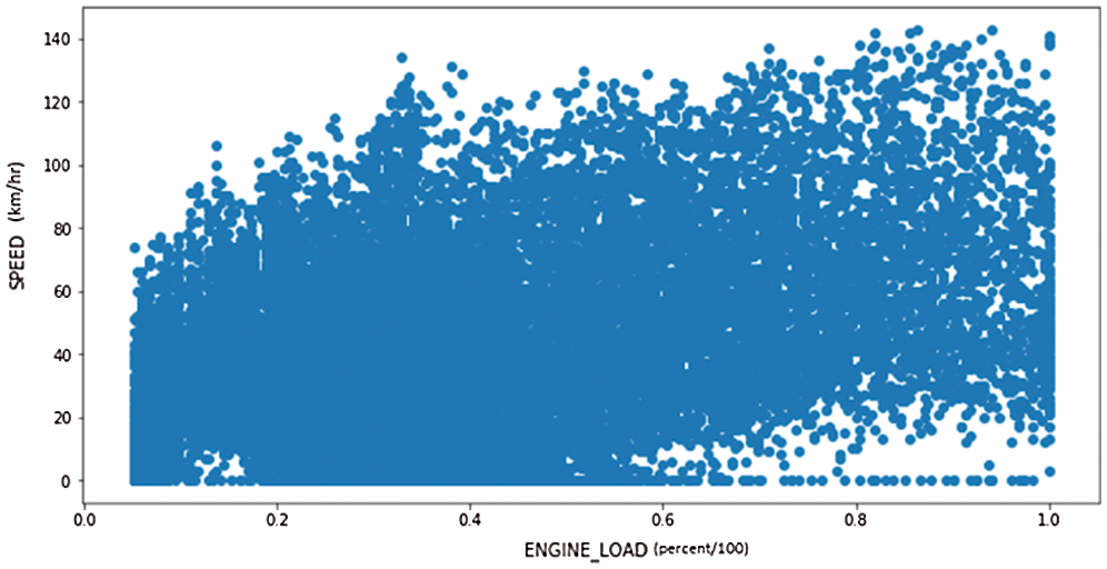
Figure 5: Instantaneous speed vs. instantaneous engine load
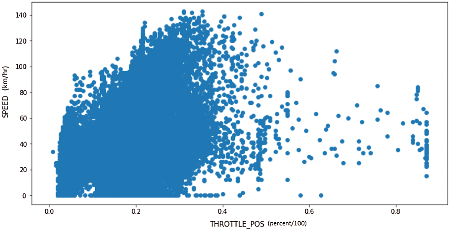
Figure 6: Instantaneous speed vs. instantaneous throttle position
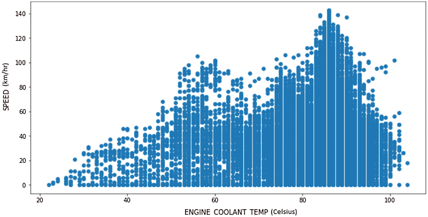
Figure 7: Instantaneous speed vs. instantaneous coolant temperature
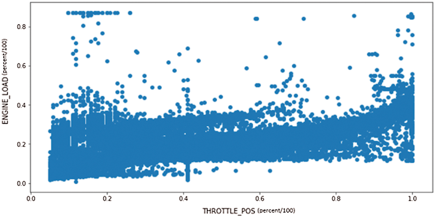
Figure 8: Instantaneous engine load vs. instantaneous throttle position
Fig. 4 illustrates a scatter plot of instantaneous speed vs. instantaneous engine rpm and it is evident that the distribution of the data points is similar to that of a straight line indicating that the two features have significant correlation between them. The other scatter plots illustrated in Figs. 5 to 8 demonstrate that different features do not show any apparent pattern or correlation between them. Fig. 9 shows a correlation map constituting of different features used in the dataset. As can be observed in the map, engine rpm and speed have a significant positive correlation. Other features do not point to any significant correlation amongst each other. A correlation plot between the features in Fig. 9 further emphasizes it by demonstrating that a correlation of 0.83 exists between these two features.
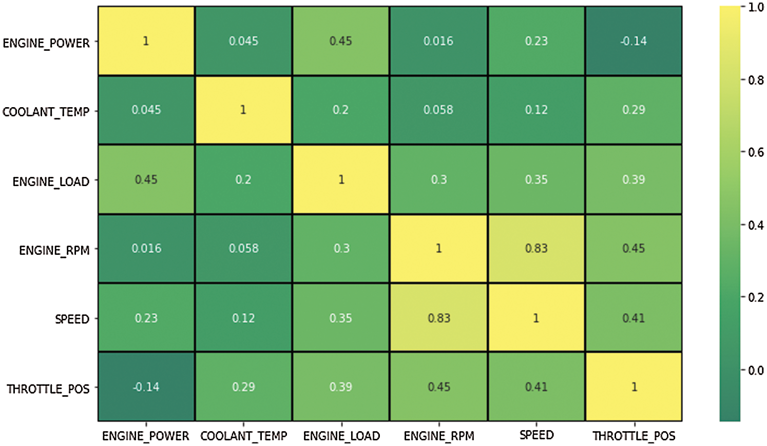
Figure 9: Correlation map of different features
After data pre-processing and cleaning, un-supervised machine learning techniques were used (further explained in the subsequent sections) in order to cluster the data points of the dataset into different groups. During unsupervised learning, the system is provided with data which is not labeled or categorized. The system is provided no prior training, therefore allowing the system to act on the data by itself. Thus, the algorithms used in this technique:
• Act on the data without any external guidance
• Attempt to understand the data and find patterns in it
• Act as a sponge on the data
Prevalent unsupervised segmentation techniques comprise of clustering (e.g., k-means, density based or hierarchical clustering), hidden Markov models [32] and feature extraction techniques like principal component analysis. Out of these techniques, the one most frequently utilized for segmentation is clustering [33]. Clustering methods are commonly used to identify groups of similar objects from a multivariate dataset. This is the most widely used technique in pattern recognition. Cluster analysis traces its roots back to the early 1960’s and was the topic of numerous studies and courses. The target of clustering is to expose subgroups within heterogeneous data such that each individual cluster has greater homogeneity than the whole [34–36].
In this research, hierarchical clustering and a centroid-based clustering technique commonly known as Lloyd’s algorithm or k-means algorithm have been used.
In data mining and statistics, hierarchical cluster [37] analysis is a clustering method used to build and analyze clusters based on hierarchy. This clustering technique involves creating groups that have a pre-determined order from top to bottom. There are two kinds of hierarchical clustering [38], Divisive and Agglomerative. The divisive clustering [39] technique involves assigning all of the observations to a single group and then dividing the group into two least similar groups. In some conditions, divisive algorithms are conceptually more complex but evidently produce hierarchies that are usually more accurate than agglomerative algorithms.
In an agglomerative clustering technique [40], each observation is assigned to its own group. Thereafter, the similarity between each of the groups is computed and similar groups are coalesced together to form a single group. This step is repeated recursively until a single group can be arrived at. Fig. 10 illustrates a dendrogram obtained as a result of running the hierarchical clustering algorithm on our dataset. The dendrogram shows that by using hierarchical clustering, the data in question can be optimally divided into two groups or clusters (green and red).

Figure 10: Dendrogram plot for hierarchical clustering
Classification of the data into sets of categories or clusters is the most significant operation with respect to the data [41]. One of several clustering methods is the technique of K-means algorithm that is run repeatedly for optimum results. The K-means technique is a modest and fundamental clustering technique which has the capability of clustering great quantities of data with rapid and effective calculation time compared to other techniques [42]. However, K-means has a drawback in that it is reliant upon the preliminary cluster center determination. K-Means cluster tests result in outcomes that are locally optimum for a given data set [43].
The K-means algorithm is an iterative algorithm that partitions the data into K predefined, distinct and non-overlapping groups. Each data point in the dataset belongs to only one of these groups. The algorithm is designed to works on making the data points within a group as similar as possible while keeping the groups as different as possible. It uses Euclidean distance to prepare clusters and group data points together. K-means follows the approach of Expectation Maximization to solve this problem. The K-means algorithm aims to minimize the square of the error function [44,45].
k signifies K cluster centers, uk signifies the kth center, and xi denotes the ith point in the data set.
In cluster analysis, in order to determine the optimal number of groups into which the data should be divided, different heuristics are used. One of the commonly deployed heuristics is the Elbow method. In this case, Within Cluster Sum of Squares (WCSS) approach is used. WCSS is a measure of the average distance of all the points within a cluster to the cluster centroid. It is a measure of how closely related the data points in a particular cluster are to the other points in the same cluster.
Fig. 11 illustrates the elbow plot, with the WCSS value on the y-axis and the number of clusters on the x-axis. As is evident from the graph, as the number of clusters created by the k-means technique increases, the WCSS value decreases exponentially. The reduction is noteworthy up until a point is touched where five clusters have been created by the algorithm. Beyond this point, the decrease in WCSS is quite negligible. This is the elbow of the curve and hence, the condition where the dataset is divided into five clusters is considered as the optimal output of the k-means algorithm.
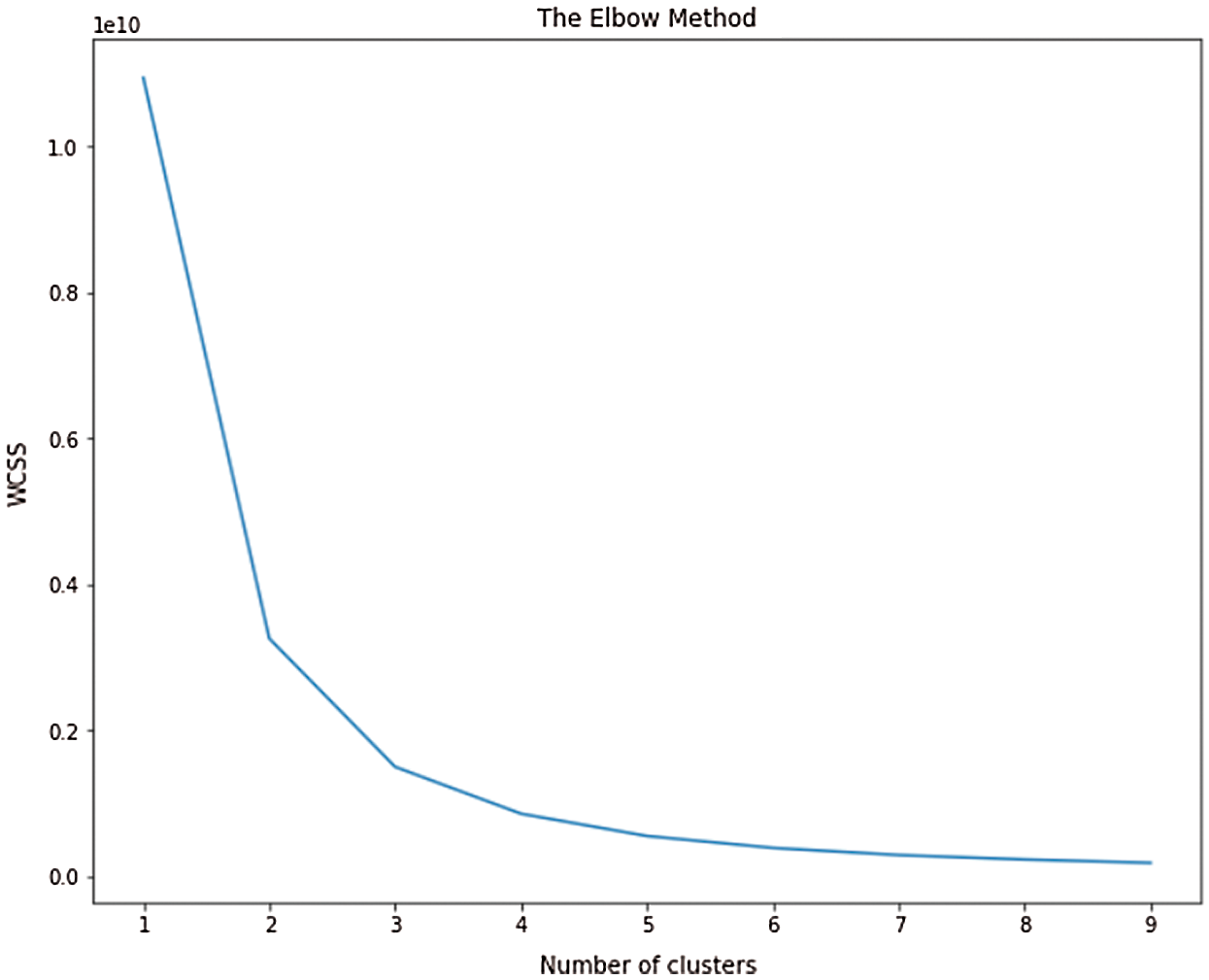
Figure 11: The Elbow plot
In order to compare the above two clustering algorithms and their respective outputs, the Davies-Bouldin Index is used. This index is an evaluation scheme which reflects and validates how well the clustering has been done and how the clusters have been formed using attributes and quantities with respect to the data. The Davies-Bouldin score is explained as the degree of similarity of each group with its most similar group. Similarity, in this case, is the ratio of within-group distances between data points to between-group distances. Thus, the farther the groups and the less dispersed they are, the better the score. On this index, lower values indicate better clustering. The lowest possible score on this index is zero.
In this research, by using the Davies-Bouldin Index, a score of 0.57 was obtained using the hierarchical clustering technique and a score of 0.52 was obtained with the k-means algorithm. Hence, the clusters created using the k-means technique were considered for further analysis. In this model, as is evident from the elbow plot, the instance is considered when the data is divided into five clusters. Subsequently, further analysis of these clusters is performed in order to understand their practical significance.
Figs. 12a to 12f represent box plots of different features and a ratio of relative rpm and relative throttle position with respect to the clusters that were created using the k-means technique. The figures show the variation of the values of the different features that were used, within the five clusters. Ignoring the outliers, it is clear that the data points in cluster 2 have a lower average and median speed while the data points that fall within cluster 3 have the highest median speed among all the clusters. Clusters 0, 1 and 4 falls between these two extremes, having median speeds that are close to each other. A similar trend is noticed across most of the features, as illustrated in Figs. 12b–12e. Fig. 12b demonstrates the distribution of engine rpm values within different clusters. As is evident from the figure, each of the clusters have distinct values for engine rpm with cluster 3 having the data points with the highest engine rpm values and cluster 2 with data points with the least engine rpm values. A ratio of relative rpm to relative throttle position is a feature that is usually used to distinguish between different driving styles and it shows a similar trend as observed in Fig. 12e.
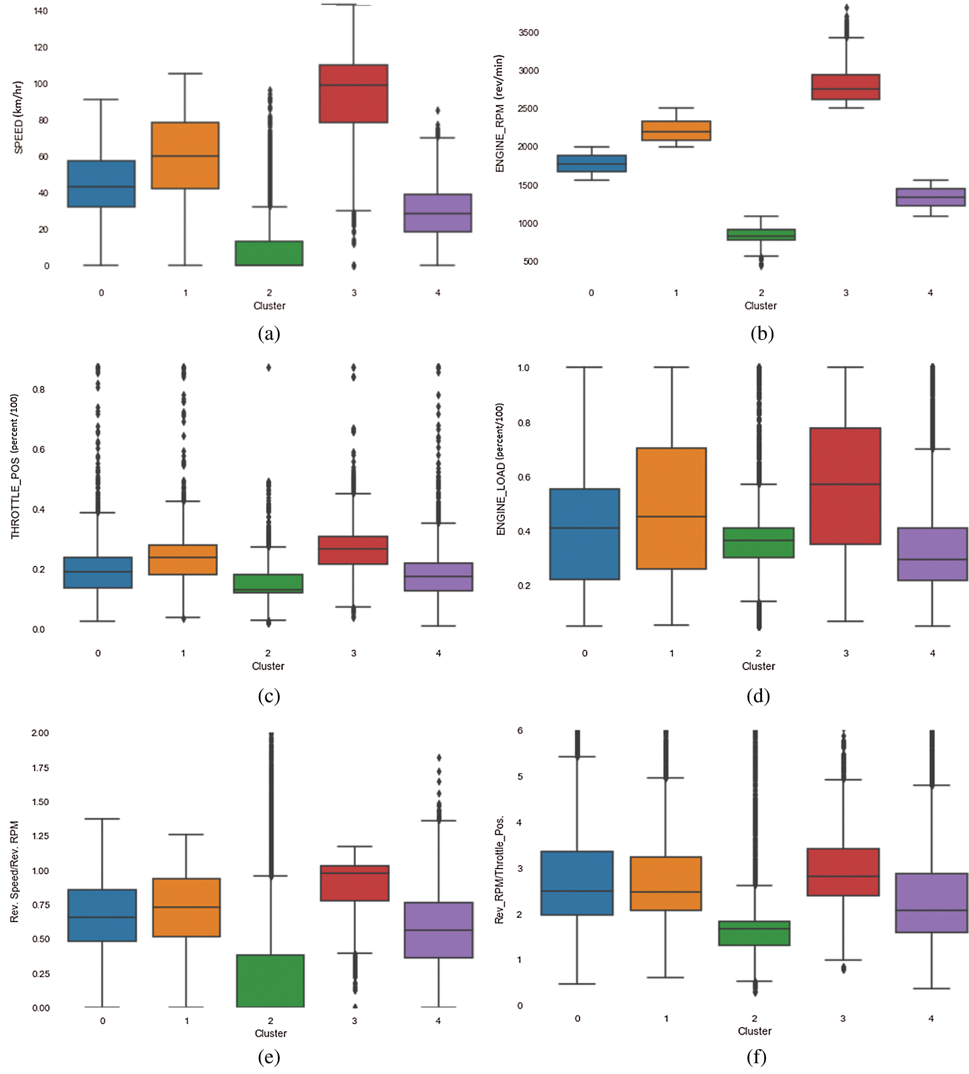
Figure 12: (a) Variation of vehicle speed within different clusters (b) Variation of engine RPM within different clusters (c) Variation of throttle position within different clusters (d) Variation of engine load within different clusters (e) Variation of the ratio of relative speed and relative RPM within different clusters (f) Variation of the ratio of relative RPM and throttle position within different clusters
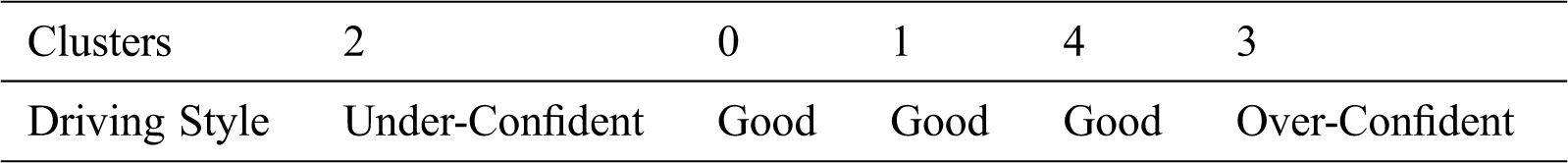
A detailed analysis of these clusters reveal that they represent different driving styles, where cluster 2 contains the data points with the lowest speed, engine RPM and throttle and represents under-confident or timid driving as it consists of data points where the vehicle speed, throttle position value etc. are much lower than the average values. Cluster 3 contains the data points with the highest average speed, engine RPM and throttle, and represents dangerous or rash driving as most of the data points in these clusters have values that are much higher than the average values of the parameters considered. Clusters 0, 1 and 4 represent driving styles that lie within these two extremes and can be considered as proper or good driving. Tab. 1 shows the driving styles represented by different clusters.
Table 1: The driving style represented by different clusters
4 Data Labeling and Supervised Techniques
The clustering technique helps in extracting driving styles and in grouping similar data points together. Upon performing a detailed analysis of the clustered data, it was concluded that that these clusters indeed represented different driving styles. These clusters were then considered as labels for the data points. Subsequently, different classification algorithms were used to train and develop a model in order to classify the data points using the cluster as the target variable.
Supervised learning techniques include a process of learning and developing a function which can map inputs to outputs on the basis of similar input/output pairs. The function is inferred using training data which is labeled or has an assigned target variable. In supervised machine learning, every data point is a pair consisting of an input value and a related output object. Supervised learning algorithms [46] produce an inferred function after analyzing training data points, and once the function has been trained, it can be used to predict the output vectors of different inputs.
4.2 Multinomial Naïve Bayes Classifier
Naïve Bayes classifiers are a type of probabilistic classifiers which are based on using the Bayes theorem, with an assumption that the features used to train the model have no correlation amongst themselves. Naïve Bayes classifiers are a generative model of supervised learning algorithms. These classifiers are fast in the way that the length of training time for these classifiers is much shorter as opposed to alternative techniques such as maximum entropy classifiers and SVMs [47,48]. Naïve Bayes classifiers fare much better in terms of consumption of computational power and memory, as demonstrated in Huang et al. [49]. Their performance is very similar to that of maximum entropy and SVM classifiers. They are typically appropriate for classifications with distinct features, as the multinomial distribution ordinarily requires integer feature counts. The Naïve Bayes algorithm forms the basis of the Multinomial Naive Bayes classifier.
A model was developed using multinomial Naïve Bayes. Fig. 13 illustrates the learning curves of the model with respect to training and test datasets. In this case, the model achieved a weighted average precision of 69% on the test dataset. This metric informs us of the overall accuracy of the trained classifier in classifying unseen data from the test dataset.
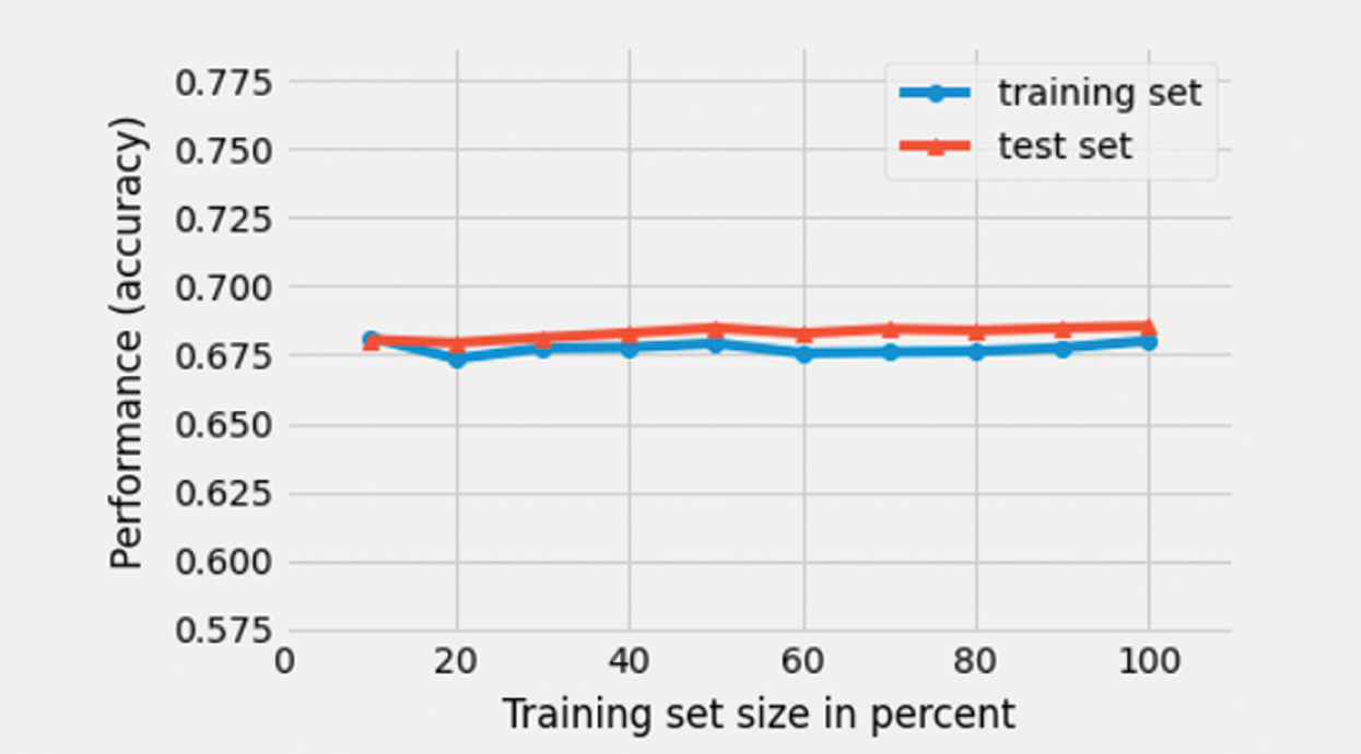
Figure 13: Learning curve of a multinomial Naïve Bayes classifier
4.3 Multinomial Logistic Regression Classifier
Logistic regression [50,51] is a statistical technique which uses a function with the same name. The logistic function lies at the core of this model. A logistic regression model is used to solve problems which can only have a finite and fixed number of outcomes. A logistic regression model assumes that there are no outliers in the data and that the features of the input data have no multi-co linearity amongst themselves. In the multinomial logistic regression technique, logistic regression in generalized to a multi-class problem, or in other words, a problem which can have more two or more distinct possible results or outcomes.
It is a statistical method for predicting a class variable and is used as a transformation technique to convert a continuous value to probabilities using a logit function (hence the name Logistic). For estimating this probability value, logistic regression uses a mathematical function known as the sigmoid function.
It has the derivative
and the indefinite integral
There may be instances where the predictions are wrong. These are errors. Just like in case of a line regression, where the least square method to get the coefficients is used such that the error is minimum, here a method called maximum likelihood is used. As in the case of linear regression, there is a cost function for logistic regression. The best separator line is the one that can generalize well on the unseen data for the purpose of label classification.
The model developed using multinomial logistic regression algorithm was trained using the training dataset and its performance was tested using the test dataset. Fig. 14 illustrates the learning curves of the mode on training and test datasets. The model was observed to achieve a weighted average precision of 85%.
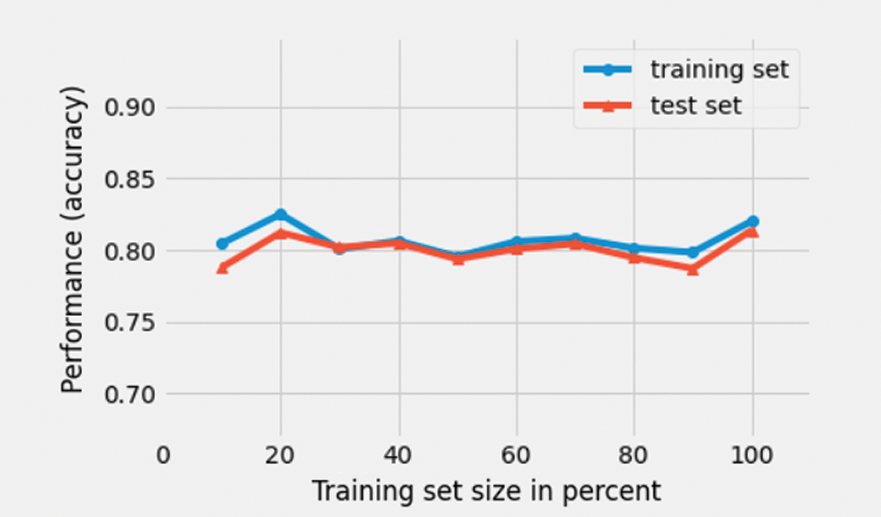
Figure 14: Learning curve of a MLR classifier
5 Neural Networks and Deep Learning
A neural network is a circuit or network of neurons or an artificial network of neurons, composed of nodes or artificial neurons. These artificial neural networks are primarily used to understand and solve complex problems that are usually tough to solve using traditional machine learning techniques. In neural network algorithms, the neural connections in an animal’s body are modeled as weights, where a weight with a positive value reflects an excitatory connection, while a weight with a negative value represents an inhibitory connection.
Deep learning (DL) [52], ML’s subdivision, has witnessed a historic resurrection in recent years, mostly compelled by an upsurge in the intensity of calculation and enormity of novel datasets. This area has recorded conspicuous improvements in the capabilities of machines in controlling and acknowledging information alongside consideration of speech [53], language [54], images [55], medication and social insurance all together, and has enormous advantage over DL due to the supreme volume of information being delivered (1018 bytes or 150 exabytes in US only, expanding 48% every year [56]). Furthermore, the growing propagation of computerized record frameworks and gadgets in clinical fields has accorded it even more currency.
Fig. 15 illustrates the mathematical representation of an artificial neuron. The values, x1, x2…xn represent the inputs coming into the neuron. The values w1, w2, ..wn represent the weights of the neuron that are multiplied with the incoming inputs. The value b represents the bias and the function g(x) is the activation function of the neuron. This activation function decides the final output of the neuron depending upon the inputs, weights and the bias. These artificial neural networks are usually utilized for predictive modeling, adaptive control and in applications where they can be trained using data.
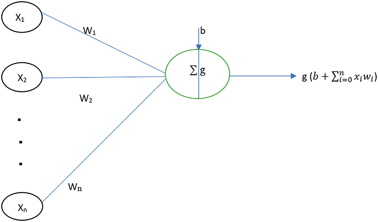
Figure 15: A neuron showing the input, corresponding weights, a bias and an activation function applied to the weighted sum of inputs
5.1 Multilayer Perceptron (Feed Forward Neural Network)
A multilayer perceptron network usually has two or more linear layers. In case of a three-layer network, the input layer is the first layer, the middle layer is the hidden layer and the final layer is what is called the output layer. Data from different features is passed to the input layer and the final output is received from the output layer. While addressing complex problems, usually more hidden layers are taken into consideration in order to get more accurate results.
In this research, MLP classifiers with hidden layer sizes 20, 40, 60 and 80 were used. The best performance was observed when the classifier had a hidden layer size of 60. Therefore, a hidden layer size of 60 was considered, first with a batch size of 16 and then with a batch size of 32. Figs. 17 and 18 represent the learning curve with accuracy, as the performance metric of two different multilayer perceptron (MLP) classifiers with batch sizes 32 and 16, respectively. As can be observed from the figure, the learning of the classifiers is seen to overall increase, as the size of the training set increases from 10% of data points in the training dataset to 100%. An accuracy of 94% and 92% was achieved on the test dataset using the MLP classifier with a batch size of 32 and 16 respectively.
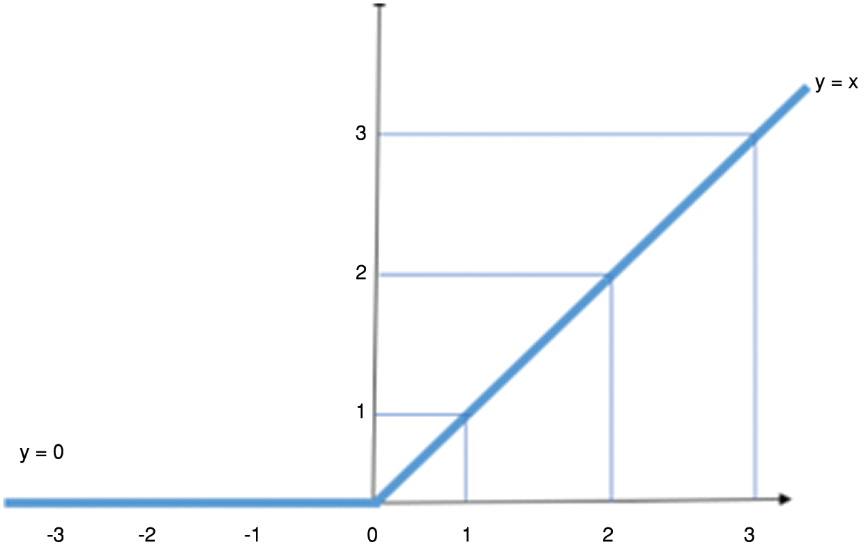
Figure 16: The ReLU activation function
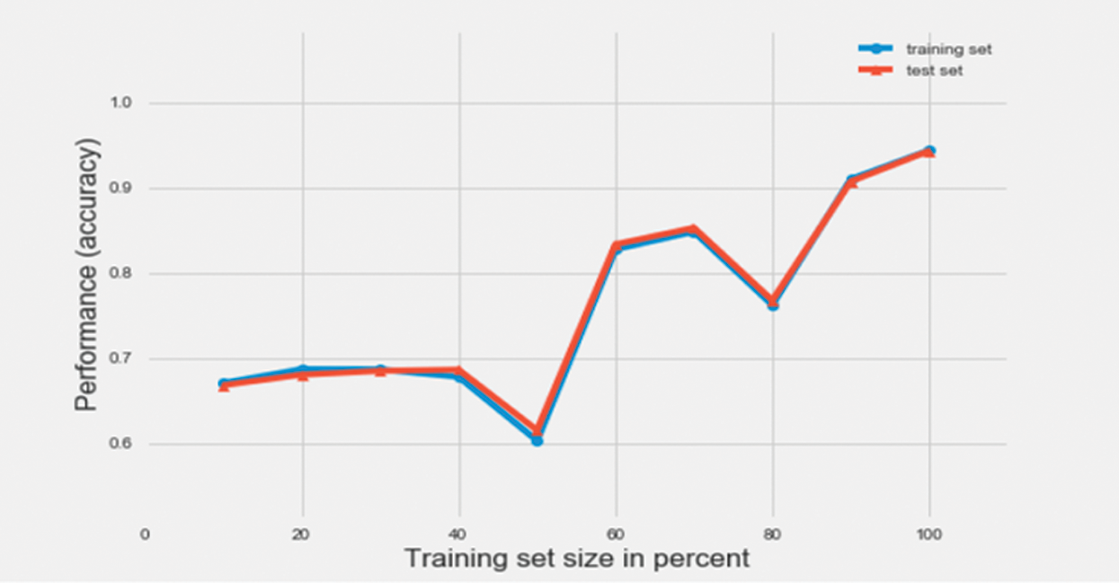
Figure 17: Learning curve of a MLP classifier with batch size 32
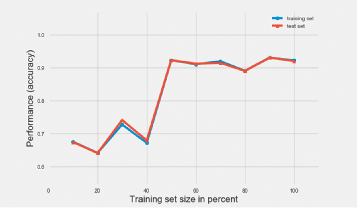
Figure 18: Learning curve of a MLP classifier with batch size 16
The output of a neural network is defined using mathematical equations which are known as activation functions. In this particular case, the Rectified Linear Unit activation function (commonly known as ReLU) has been used. Fig. 16 demonstrates a graphical representation of the ReLU function. ReLU is mathematically defined as y = max (0, x). This clearly indicates that the output value of the function is equal to the input for all values greater than zero and the output of the function is zero for all non-positive values of the input.
5.2 Artificial Neural Networks
ANN was first proposed in 1943 by a neurophysiologist, Warren McCulloch and a mathematician, Walter Pitts. Perceptrons and artificial neural networks are different and one major point of difference is that, in a common perceptron, the function that spits out the output, is usually a step function. Neural networks have evolved from MLPs which can use different kinds of activation functions. The activation function used in particular cases depends upon the kind of output expected from the network. Fig. 19 represents the change in the value of loss function with the increase in the number epochs. The loss function that was used in this study is the categorical cross entropy function. This function is used when the output is in categorical form and only one result can be correct. Categorical cross entropy function compares the distribution of the predictions with the true distribution, where the probability of the correct group or cluster is set to 1 and 0 for the other groups.
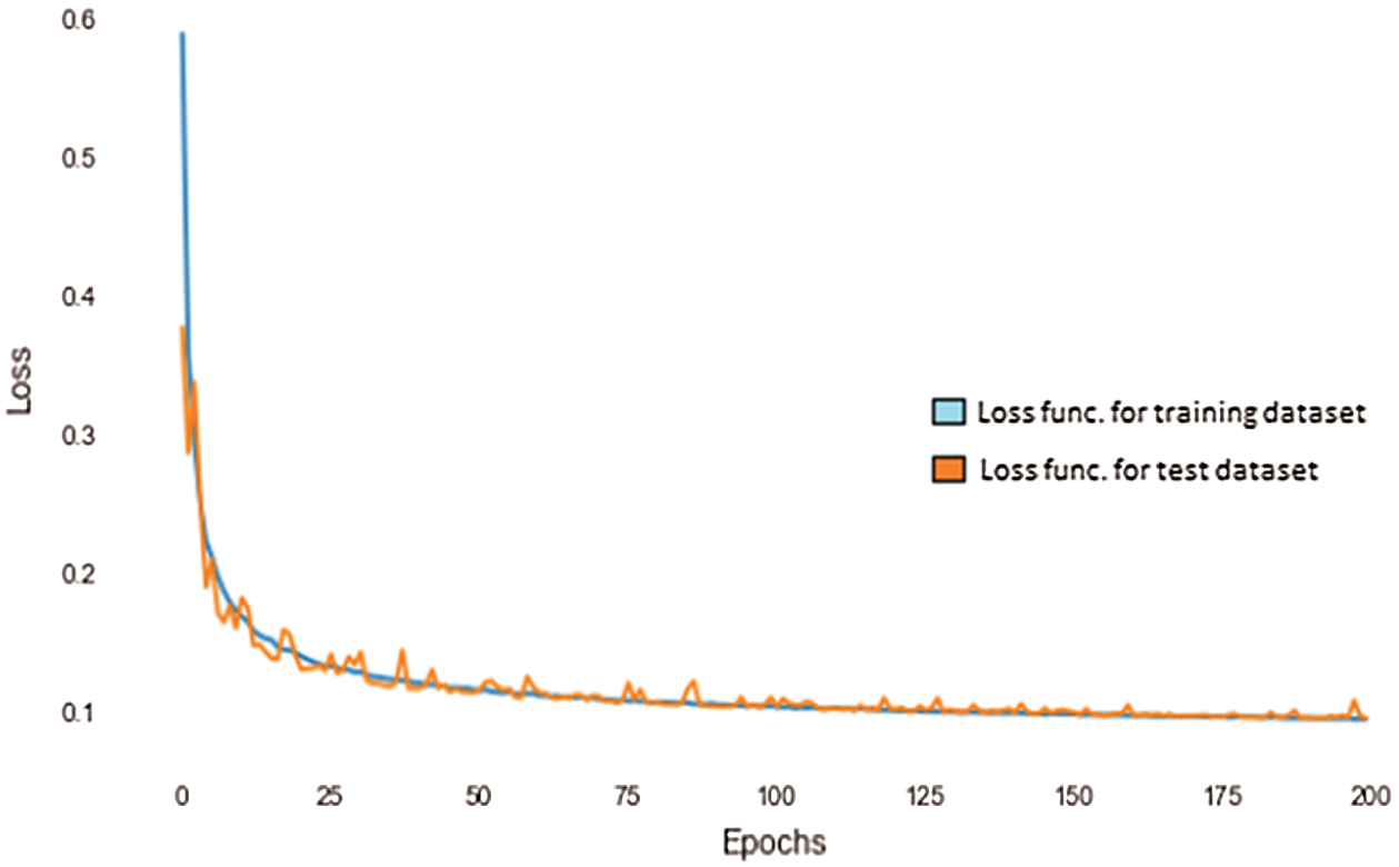
Figure 19: Loss vs. Epochs curve using ANN
The blue curve in the figure represents the change in the loss function for the training dataset against the number of epochs and the orange curve represents the change in the value of the loss function for the test dataset in question. As can be observed from the graph, the value of the loss function falls steeply as the number of epochs increases, both in the case of the training as well as the test datasets.
Fig. 20 demonstrates the accuracy of the ANN classifier against the number of epochs. The blue curve represents the accuracy for the training dataset and the orange curve represents the accuracy for the test dataset. As can be seen from the figure, the accuracy achieved by the classifier increases with the number of epochs and reaches almost 99% at about 200 epochs.
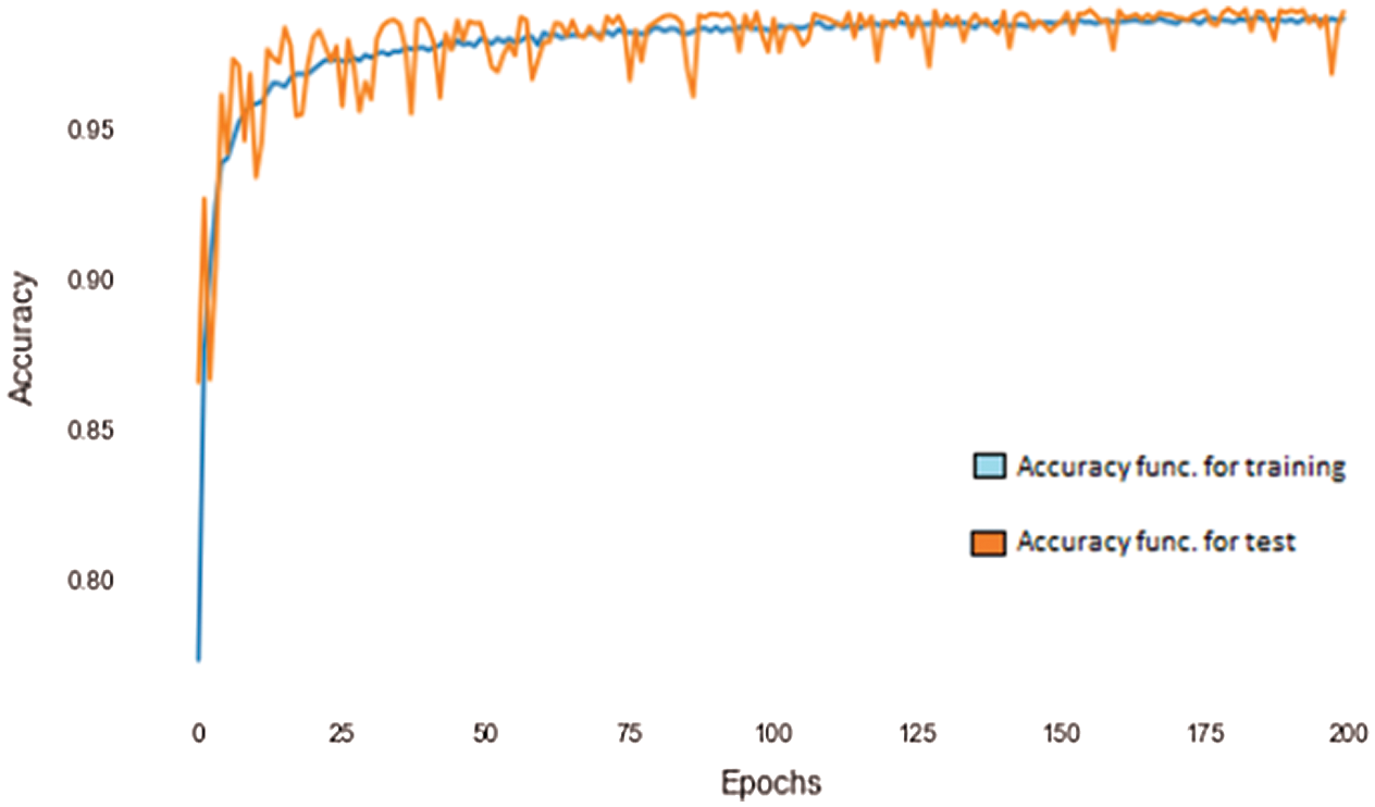
Figure 20: Accuracy vs. Epochs curve using ANN
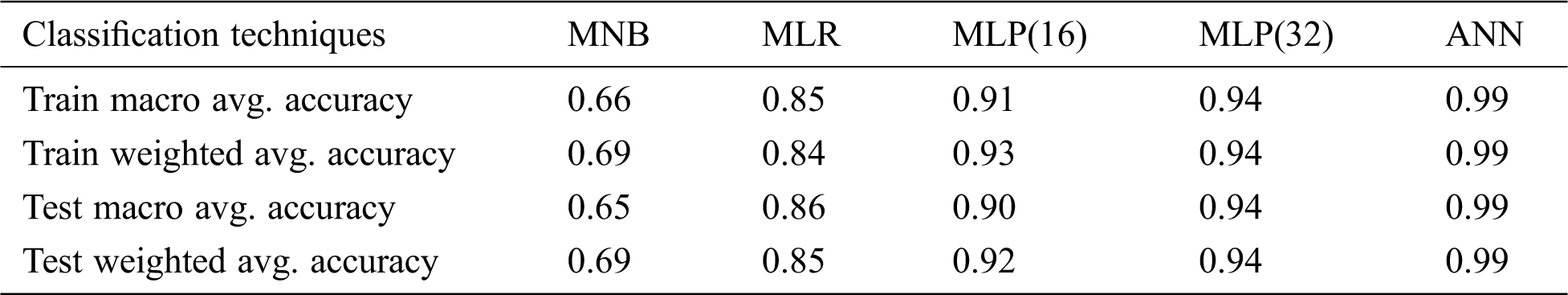
In this case, an ANN with four layers was used with one input and one output layer and two hidden layers. As is evident from Figs. 19 and 20, the accuracy of the classifier increased with the number of epochs and at 200 epochs, an accuracy of 99% was achieved. Different classifiers and the respective precisions achieved are compared in Tab. 2.
Table 2: Comparison of accuracy rates using different classifiers
This research proposes a model which can be used to understand driving data and extract driving patterns in order to classify the data into different groups, to ultimately enable insightful and relevant action. The data for this purpose was collected from the OBD port of a vehicle. The data was at first pre-processed and then pattern mining techniques were used to extract patterns from this data. Upon further studying and analyzing the clusters that were created, it was confirmed that they represented distinct driving patterns. These clusters were then used as labels and different advanced techniques and algorithms were used to develop a classifier which could accurately classify the data points into the corresponding groups or clusters. Using deep learning techniques, an accuracy of 99% was achieved in the classification undertaken, thus demonstrating that this model can be used in real-life products and implementations. The primary aim of this research was to develop and present a model which can be used to identify different driving patterns from the data and classify the incoming data into different groups accurately. This model can also be used in fleet management systems to monitor driving styles.
In this research, work was limited to the data obtained from the on-board diagnostics of the vehicles. In future work, external sensors like 3-axis accelerometers and gyroscopes can also be used in inclusion with the data coming from the OBD board. This data could help in providing more insights about the driving patterns of a driver on a particular route. Data from accelerometers and gyroscopes can be used to understand the condition of the routes (good/damaged roads with potholes and speed breakers).
This could help in further understanding real life conditions on the roads, like the movement of traffic during traffic jams, working hours, holidays, weekends etc. This would ultimately help in tuning the presented model for better predictions. This could also help in making a profile of a particular driver and in understanding his/her driving style in a better way in order to institute or reinforce any relevant training or action. This data can also be used in the development of a model to predict the fuel efficiency of a vehicle with respect to the driving style.
Funding Statement: The authors received no specific funding for this study.
Conflicts of Interest: The authors declare that they have no conflicts of interest to report regarding the present study.
1. Y. J. Pan, T. C. Yu and R. S. Cheng, “Using OBD-II data to explore driving behavior model,” in 2017 Int. Conf. on Applied System Innovation (ICASISapporo, Japan, pp. 1816–1818, 2017. [Google Scholar]
2. H. Rowen and K. DiBiasio, “The insurance coverage implications of using a cell phone app to hail a ride,” Brief, vol. 44, no. 12, pp. 12–23, 2014. [Google Scholar]
3. Q. Xu, B. Wang, F. Zhang, D. S. Regani, F. Wang et al., “Wireless AI in smart car: How smart a car can be?,” IEEE Access, vol. 8, pp. 55091–55112, 2020. [Google Scholar]
4. M. Amarasinghe, S. Kottegoda, A. L. Arachchi, S. Muramudalige, H. D. Bandara et al., “Cloud-based driver monitoring and vehicle diagnostic with OBD2 telematics,” in 2015 Fifteenth Int. Conf. on Advances in ICT for Emerging Regions (ICTerColombo, Sri Lanka, pp. 243–249, 2015. [Google Scholar]
5. Y. Kishimoto and K. Oguri, “A modeling method for predicting driving behavior concerning with drivers pastmovements,” in IEEE Int. Conf. on Vehicular Electronics and Safety (IEEE ICVES 2008Columbus Ohio, USA, pp. 132–136, 2008. [Google Scholar]
6. R. H. Osgouei and S. Choi, “Evaluation of driving skills using an HMM-based distance measure,” in 2012 IEEE Int. Workshop on Haptic Audio-Visual Environments and Games (HAVE 2012) Proc., Munich, Germany, pp. 50–55, 2012. [Google Scholar]
7. V. Vaitkus, P. Lengvenis and G. Žylius, “Driving style classification using long-term accelerometer information,” in 2014 19th Int. Conf. on Methods and Models in Automation and Robotics (MMARSzczecin, Poland, pp. 641–644, 2014. [Google Scholar]
8. M. Fazeen, B. Gozick, R. Dantu, M. Bhukhiya and M. C. Gonzalez, “Safe driving using mobile phones,” IEEE Transactions on Intelligent Transportation Systems, vol. 13, no. 3, pp. 1462–1468, 2012. [Google Scholar]
9. J. Dai, J. Teng, X. Bai, Z. Shen and D. Xuan, “Mobile phone based drunk driving detection,” in 2010 4th Int. Conf. on Pervasive Computing Technologies for Healthcare, Munich, Germany: IEEE, pp. 1–8, 2010. [Google Scholar]
10. M. R. Othman, Z. Zhang, T. Imamura and T. Miyake, “A study of analysis method for driver features extraction,” in IEEE Int. Conf. on Systems, Man and Cybernetics, pp. 12–15, 2008. [Google Scholar]
11. Y. L. Murphey, R. Milton and L. Kiliaris, “Drivers style classification using jerk analysis,” in IEEE Sym. on Computational Intelligence in Vehicles and Vehicular Systems, Nashville, TN, USA, pp. 23–28, 2009. [Google Scholar]
12. T. Lotan and T. Toledo, “Evaluating the safety implications and benefits of an in-vehicle data recorder to young drivers,” in Proc. of the 3rd Int. Driving Sym. on Human Factors in Driver Assessment, Training, and Vehicle Design, Rockport Maine, United States, pp. 448–455, 2005. [Google Scholar]
13. B. R. Cooper and K. McClelland, “Event data recorders: Balancing the benefits and drawbacks,”IRMI, 2008. [Online]. Available at: https://www.irmi.com/articles/expert-commentary/event-data-recorders-balancing-the-benefits-and-drawbacks. [Google Scholar]
14. J. Zhang, Z. Wu, F. Li, C. Xie, T. Ren et al., “A deep learning framework for driving behavior identification on in-vehicle CAN-BUS sensor data,” Sensors, vol. 19, no. 6, pp. 1356, 2019. [Google Scholar]
15. M. L. Bernardi, M. Cimitile, F. Martinelli and F. Mercaldo, “Driver and path detection through time-series classification,” Journal of Advanced Transportation, vol. 2018, no. 3, pp. 1–20, 2018. [Google Scholar]
16. S. Choi, J. Kim, D. Kwak, P. Angkititrakul and J. H. Hansen, “Analysis and classification of driver behavior using in-vehicle can-bus information, ” in Biennial workshop on DSP for In-Vehicle and Mobile Systems, pp. 17–19, 2007. [Google Scholar]
17. C. Miyajima, Y. Nishiwaki, K. Ozawa, T. Wakita, K. Itou et al., “Driver modeling based on driving behavior and its evaluation in driver identification,” Proceedings of the IEEE, vol. 95, no. 2, pp. 427–437, 2007. [Google Scholar]
18. J. Ferreira, E. Carvalho, B. V. Ferreira, C. de Souza, Y. Suhara et al., “Driver behavior profiling: An investigation with different smartphone sensors and machine learning,” PLoS One, vol. 12, no. 4, pp. e0174959, 2017. [Google Scholar]
19. Y. Sun, H. Song, A. J. Jara and R. Bie, “Internet of things and big data analytics for smart and connected communities,” IEEE Access, vol. 4, pp. 766–773, 2016. [Google Scholar]
20. J. Engelbrecht, M. J. Booysen, G. J. van Rooyen and F. J. Bruwer, “Survey of smartphone-based sensing in vehicles for intelligent transportation system applications,” IET Intelligent Transport Systems, vol. 9, no. 10, pp. 924–935, 2015. [Google Scholar]
21. R. Malekian, N. R. Moloisane, L. Nair, B. T. Maharaj and U. A. Chude-Okonkwo, “Design and implementation of a wireless OBD II fleet management system,” IEEE Sensors Journal, vol. 17, no. 4, pp. 1154–1164, 2017. [Google Scholar]
22. A. Pal and M. Pal, “IoT for vehicle simulation system,” Int. Journal of Engineering Science, vol. 7, no. 2, pp. 1–4, 2017. [Google Scholar]
23. A. Ahire, V. Baviskar, P. Khairnar, S. Jadhav and D. Shisode, “Web based fuel statistic monitoring for automobiles,” Int. Journal of Engineering Science, vol. 10, pp. 1–4, 2017. [Google Scholar]
24. F. N. Ogwueleka, S. Misra, T. C. Ogwueleka and L. Fernandez-Sanz, “An artificial neural network model for road accident prediction: a case study of a developing country,” Acta Polytechnica Hungarica, vol. 11, no. 5, pp. 177–197, 2014. [Google Scholar]
25. M. JinKim, J. WookJang and Y. S. Yu, “A study on in-vehicle diagnosis system using OBD-II with navigation,” Int. Journal of Computer Science and Network Security, vol. 10, no. 9, pp. 136–140, 2010. [Google Scholar]
26. V. Asha, N. U. Reddy and N. Awasthi, “A novel approach to monitor and analyze the usage and prediction of requirement of fuel for cluster of generator sets,” in 2016 Int. Conf. on Inventive Computation Technologies (ICICTCoimbatore, Tamilnadu, India, 2, pp. 1–4, 2016. [Google Scholar]
27. B. N. K. Kumar and M. V. P. Rao, “A novel cognitive security approach for internet of things,” International Journal of Engineering and Technology, vol. 9, no. 3S, pp. 579–584, 2017. [Google Scholar]
28. M. D. Pesé, A. Ganesan and K. G. Shin, “Carlab: Framework for vehicular data collection and processing,” in Proc. of the 2nd ACM Int. Workshop on Smart, Autonomous, and Connected Vehicular Systems and Services, New York, USA, pp. 43–48, 2017. [Google Scholar]
29. S. H. Baek and J. W. Jang, “Implementation of integrated OBD-II connector with external network,” Information Systems, vol. 50, pp. 69–75, 2015. [Google Scholar]
30. M. Zhang, R. Chen, X. Zhang, Z. Feng, G. Rao et al., “Intelligent RDD management for high performance in-memory computing in spark,” in Proc. of the 26th Int. Conf. on World Wide Web Companion, Perth, Australia, pp. 873–874, 2017. [Google Scholar]
31. X. Ma, Z. Dai, Z. He, J. Ma, Y. Wang et al., “Learning traffic as images: a deep convolutional neural network for large-scale transportation network speed prediction,” Sensors, vol. 17, no. 4, pp. 1–16, 2017. [Google Scholar]
32. S. Liu, K. Zheng, L. Zhao and P. Fan, “A driving intention prediction method based on hidden Markov model for autonomous driving,” Computer Communications, vol. 157, no. 2, pp. 143–149, 2020. [Google Scholar]
33. V. Badrinarayanan, I. Budvytis and R. Cipolla, “Semi-supervised video segmentation using tree structured graphical models,” IEEE Transactions on Pattern Analysis and Machine Intelligence, vol. 35, no. 11, pp. 2751–2764, 2013. [Google Scholar]
34. E. Bijnen, P. Stouthard and C. Brand-Maher, Cluster analysis: Survey and evaluation of techniques. Springer Netherlands: Springer Science & Business Media, 2012. [Google Scholar]
35. P. K. Amalaman, C. F. Eick and C. Wang, “Supervised taxonomies - algorithms and applications,” IEEE Transactions on Knowledge and Data Engineering, vol. 29, no. 9, pp. 2040–2052, 2017. [Google Scholar]
36. Y. Liang and J. D. Lee, “A hybrid Bayesian network approach to detect driver cognitive distraction,” Transportation Research Part C: Emerging Technologies, vol. 38, no. 6, pp. 146–155, 2014. [Google Scholar]
37. S. C. Johnson, “Hierarchical clustering schemes,” Psychometrika, vol. 32, no. 3, pp. 241–254, 1967. [Google Scholar]
38. M. S. G. Karypis, V. Kumar and M. Steinbach, “A comparison of document clustering techniques, ” in Text Mining Workshop at KDD 2000. Boston, USA, pp. 1–20, 2000. [Google Scholar]
39. D. Boley, “Principal directions divisive partitioning,” Data Mining and Knowledge Discovery, vol. 2, no. 4, pp. 325–344, 1998. [Google Scholar]
40. H. E. D. William and H. Edelsbrunner, “Efficient algorithms for agglomerative hierarchical clustering methods,” Journal of Classification, vol. 1, no. 1, pp. 7–24, 1984. [Google Scholar]
41. K. M. Bataineh, M. Naji and M. Saqer, “A comparison study between various fuzzy clustering algorithms,” Jordan Journal of Mechanical and Industrial Engineering (JJMIE), vol. 5, no. 4, pp. 335–343, 2011. [Google Scholar]
42. B. K. Khotimah, F. I. R. L. I. Irhamni and T. R. I. Sundarwati, “A genetic algorithm for optimized initial centers k-means clustering in SMEs,” Journal of Theoretical and Applied Information Technology, vol. 90, no. 1, pp. 23–30, 2016. [Google Scholar]
43. F. Marisa, S. S. S. Ahmad, Z. I. M. Yusof, F. Hunaini and T. M. A. Aziz, “Segmentation model of customer lifetime value in small and medium enterprise (SMEs) using K-means clustering and LRFM model,” International Journal of Integrated Engineering, vol. 11, no. 3, pp. 169–180, 2019. [Google Scholar]
44. Y. Li and H. Wu, “A clustering method based on K-means algorithm,” Physics Procedia, vol. 25, no. 1, pp. 1104–1109, 2012. [Google Scholar]
45. S. Na, L. Xumin and G. Yong, “Research on k-means clustering algorithm: An improved k-means clustering algorithm,” in 2010 Third Int. Sym. on Intelligent Information Technology and Security Informatics, NW Washington, DC, USA, pp. 63–67, 2010. [Google Scholar]
46. P. Cunningham, M. Cord and S. J. Delany, “Supervised learning, ” in Machine Learning Techniques for Multimedia, Springer, pp. 21–49,2008. [Google Scholar]
47. T. Evgeniou and M. Pontil, “Support vector machines: Theory and applications,” in Advanced Course on Artificial Intelligence, Springer, pp. 249–2571999. [Google Scholar]
48. V. Kecman and L. Wang, “Support Vector Machines: Theory and Applications,” Vol. 177. Berlin, Heidelberg: Springer, 2005. [Google Scholar]
49. J. Huang, J. Lu and X. C., “Ling Comparing Naive Bayes, decision trees, and SVM with AUC and accuracy,” in Third IEEE Int. Conf. on Data Mining, NW Washington, DC, USA: IEEE, pp. 553–556, 2003. [Google Scholar]
50. Y. H. Chan, “Biostatistics,” Logistic Regression Analysis, vol. 46, no. 6, pp. 259, 2005. [Google Scholar]
51. A. Bayaga, “Multinomail logistic regression: Usage and application in risk analysis,” Journal of Applied Quantitative Methods, vol. 5, no. 2, pp. 288–297, 2010. [Google Scholar]
52. A. S. Al-Waisy, M. A. Mohammed, S. Al-Fahdawi, M. S. Maashi, B. Garcia-Zapirain et al., “Covid-deepnet: hybrid multimodal deep learning system for improving covid-19 pneumonia detection in chest x-ray images,” Computers, Materials & Continua, vol. 67, no. 2, pp. 2409–2429, 2021. [Google Scholar]
53. O. Russakovsky, J. Deng, H. Su, J. Krause, S. Satheesh et al., “Imagenet large scale visual recognition challenge,” International Journal of Computer Vision, vol. 115, no. 3, pp. 211–252, 2015. [Google Scholar]
54. M. A. Mohammed, K. H. Abdulkareem, B. Garcia-Zapirain, S. A. Mostafa, M. S. Maashi et al., “A comprehensive investigation of machine learning feature extraction and classification methods for automated diagnosis of covid-19 based on x-ray images,” Computers, Materials & Continua, vol. 66, no. 3, pp. 3289–3310, 2021. [Google Scholar]
55. P. T. Nguyen, V. Dang, K. D. Vo, P. T. Phan, M. Elhoseny et al., “Deep learning based optimal multimodal fusion framework for intrusion detection systems for healthcare data,” Computers Materials & Continua, vol. 66, no. 3, pp. 2555–2571, 2021. [Google Scholar]
56. L. Minor, “Harnessing the power of data in health, Stanford Med,” Health Trends Report, Stanford Medicine, 2017. [Google Scholar]
 | This work is licensed under a Creative Commons Attribution 4.0 International License, which permits unrestricted use, distribution, and reproduction in any medium, provided the original work is properly cited. |