DOI:10.32604/iasc.2021.016990
| Intelligent Automation & Soft Computing DOI:10.32604/iasc.2021.016990 | |
| Article |
A New Estimation of Nonlinear Contact Forces of Railway Vehicle
1NCRA-Condition Monitoring Systems Lab, Mehran University of Engineering & Technology, Jamshoro, Pakistan
2Department of Electronic Engineering Mehran University of Engineering & Technology, Jamshoro, Pakistan
3DHA Suffa University, Karachi, 75500, Pakistan
4School of Information Technology and Engineering Melbourne Institute of Technology, Melbourne, Australia
5Faculty of Computing and Informatics University Malaysia Sabah, Kota Kinabalu, 88400, Malaysia
6Department of Electronics and Communication Engineering, JECRC University, Vidhani, Jaipur, 303905, India
*Corresponding Author: Kashif Nisar. Email: Kashif@ums.edu.my
Received: 17 January 2021; Accepted: 21 February 2021
Abstract: The core part of any study of rolling stock behavior is the wheel-track interaction patch because the forces produced at the wheel-track interface govern the dynamic behavior of the whole railway vehicle. It is significant to know the nature of the contact force to design more effective vehicle dynamics control systems and condition monitoring systems. However, it is hard to find the status of this adhesion force due to its complexity, highly non-linear nature, and also affected with an unpredictable operation environment. The purpose of this paper is to develop a model-based estimation technique using the Extended Kalman Filter (EKF) with inertial sensors to estimate non-linear wheelset dynamics in variable adhesion conditions. The proposed model results show the robust performance of the EKF algorithm in dry, wet/rain, greasy, and fully contaminated track conditions in traction and braking modes of a railway vehicle. The proposed model is related to the other works in the area of wheel-rail systems and a tradeoff exists in all conditions. This model is very useful in condition monitoring systems for railway asset management to avoid accidents and derailment of a train.
Keywords: Extended Kalman filter; railway dynamics; wheel-rail interface
The rapid development in railway traffic across the world demands better acceleration and braking performance. The railway wheelset and wheel-rail contact patch play a vital role in the acceleration and braking performance of railway operation [1]. In the railway operational terminology, the transmitted tangential force between wheel and rail is called adhesion force [2]. At wheel-rail contact patch, a certain level of adhesion force is necessary for the transfer of tractive force applied by traction and braking network in locomotives. The exerted tractive force may exceed the highest adhesion level present at the wheel-track contact, causing the occurrence of wheel slip in acceleration and skid in braking [3]. This wheel slip and slide largely affects routine railway operations. Mainly, it increases maintenance cost, undesirable wear of both wheel and track surfaces, and increases safety risk. As adhesion force or creep force changes non-linearly to slip ratio and is affected by the unpredictable variations in wheel-rail contact conditions. The wheel-rail contact conditions are usually categorized into four types based on external contaminantes: (i) Dry track or normal adhesion condition, (ii) Wet track or bad adhesion condition, (iii) Oily/Greasy track or poor adhesion condition and (iv) Fully contaminated track or extremely slippery adhesion condition. Some images of contaminated track and wheel-rail contact captured during field visit are illustrated in Fig. 1.
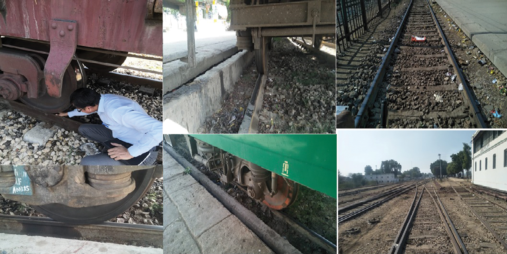
Figure 1: Visited railway track and wheel-rail contact
The estimation of adhesion coefficient, slip ratio, and lateral dynamics of railway vehicle successively in traction and braking modes is essential for both trip safety and passenger ease. But estimation of wheelset dynamics is a complicated process because the wheel-rail interface is an open system with changing external conditions. Many scholars have proposed some wheel-rail contact estimation techniques most of which are model-based, which have been summarized in Refs. [2,4,5]. For example in Hussain et al. [6], adhesion limit is identified by using a bank of Kalman filters and a Fuzzy logic system. However, the use of multiple Kalman filters makes the computation complex and difficult to apply to a real system. A model-based estimation technique using EKF is proposed in Zhao et al. [7] to detect slip-slide indirectly by measuring parameters of the traction motor. Another work presented by Zhao et al. [8] is to use Unscented Kalman filter for estimating creep, creep force, and friction coefficient from the behavior of the traction motor. A two-dimensional inverse wagon model based on acceleration is developed in Sun et al. [9] for assessment and monitoring of wheel-rail contact dynamics forces. The results at higher speed are agreeable, however, improvement in the model is further needed to reduce the error at all expected speeds. In Strano et al. [10], wheel-rail nonlinear contact forces and moments are estimated on model-based using EKF. But the technique is not verified on all adhesion conditions. In Mal et al. [11] model-based estimation technique using EKF is proposed for estimation of contact force and other lateral wheelset dynamics but the proposed technique is not suitable for traction and braking modes of railway vehicle operation. One data-driven method based on particle swarm optimization (PSO) and kernel extreme learning machine (KELM) is proposed in Liu et al. [12] to identify wheel/rail adhesion of heavy-haul locomotives. But the method is just verified in dry track conditions, so further work is needed to estimate adhesion state in wet, greasy, and extremely slippery tracks. Another work related to the data-driven approach using Deep Neural Network is proposed in Ujjan et al. [13] to identify wheel-rail contact conditions. In Zirek [14], a swarm intelligence-based adhesion estimation algorithm is proposed for an effective anti-slip control system but for low adhesion conditions it cannot estimate correctly. Track irregularities are also estimated in Munoz et al. [15] by a model-based technique using the Kalman filtering algorithm. Traction force is estimated in Ishrat et al. [16] by using the Kalman filtering algorithm for further designing slip controllers.
Several methods have been proposed in the literature to accurately estimate the adhesion condition in railway transport. Most of these techniques are designed to work during the normal operation (steady-state) of a railway vehicle. Accurate adhesion information is not only important during the normal running conditions, it is also important during the traction and braking modes to avoid wheel-slip during traction and wheel-slide during braking. But due to the highly nonlinear behavior of the wheelset dynamics during the traction and braking modes, it is very difficult to accurately estimate the adhesion condition. In addition to the presence of nonlinearities during the traction and braking modes, the unpredictable environmental conditions present a serious challenge for researchers to accurately estimate adhesion at the wheel-rail interface. In this paper, we extend the works reported in Refs. [6,11], by design and development of the extended Kalman filter model for estimation of adhesion coefficient, slip ratio, and wheelset lateral dynamics in both traction and braking modes of vehicle operation by taking all track conditions. The rest of the paper proceeds as follows. Section 2 presents the modeling of the wheelset and in Section 3 design of the estimator is described. In Section 4 simulation results are discussed and lastly, Section 5 is about the conclusion and future work.
2 Modeling of Railway Wheelset
This research work focuses on the extension of the railway wheelset dynamics as reported in Refs. [6,11]. In this section, a comprehensive model of the wheelset, motion equations of the wheelset, and creep curves for all adhesion conditions are presented. A complete and accurate wheelset model is required to validate the proposed estimation technique. Hence, a conventional solid axle wheelset shown in Fig. 2 is taken to demonstrate the potential of the proposed idea.
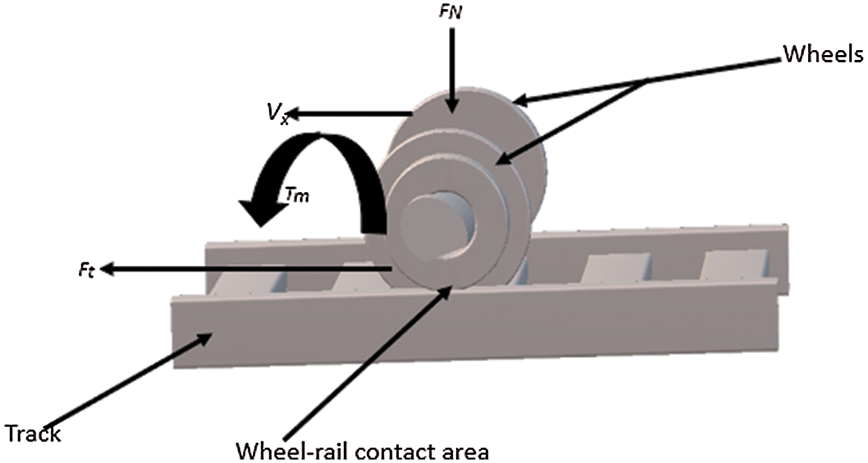
Figure 2: Railway wheelset model
In the above figure torque (Tm) of traction motor attached on one side of the wheelset, traction force (Ft), the normal force (FN), and linear velocity (Vx) are labeled being important parameters involved in modeling.
The Adhesion coefficient is one of the most important parameters of wheelset because the dynamic response of the wheelset depends on it. The adhesion coefficient
In normal condition with small slip ratio, the adhesion force is linear with slip ratio but for the large slip ratio the adhesion force becomes nonlinear and can be expressed as:
where j = longitudinal and lateral directions.
The total tangential force Fa of longitudinal and lateral directions can be calculated using the Polach formula [17] as:
where kA is the reduction factor around adhesion, KS is the reduction factor in a slip,
where
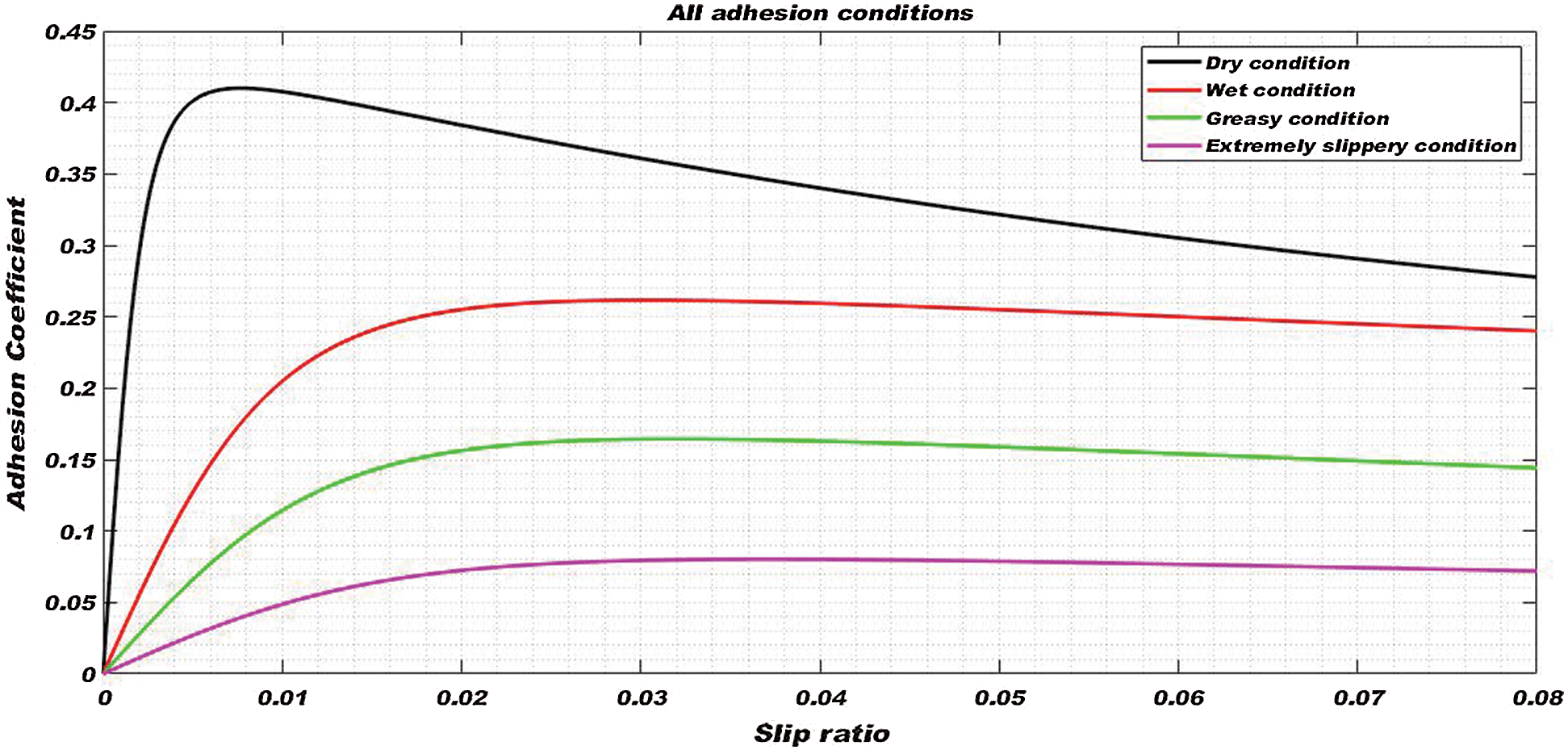
Figure 3: Creep curves for all adhesion conditions
Each curve can be divided into three parts to describe the stable and unstable behavior of the wheelset. The initial portion is almost linear, the middle portion is nonlinear and is called the high slip ratio region and the last portion having a negative slope is the unstable region of the curve [3].
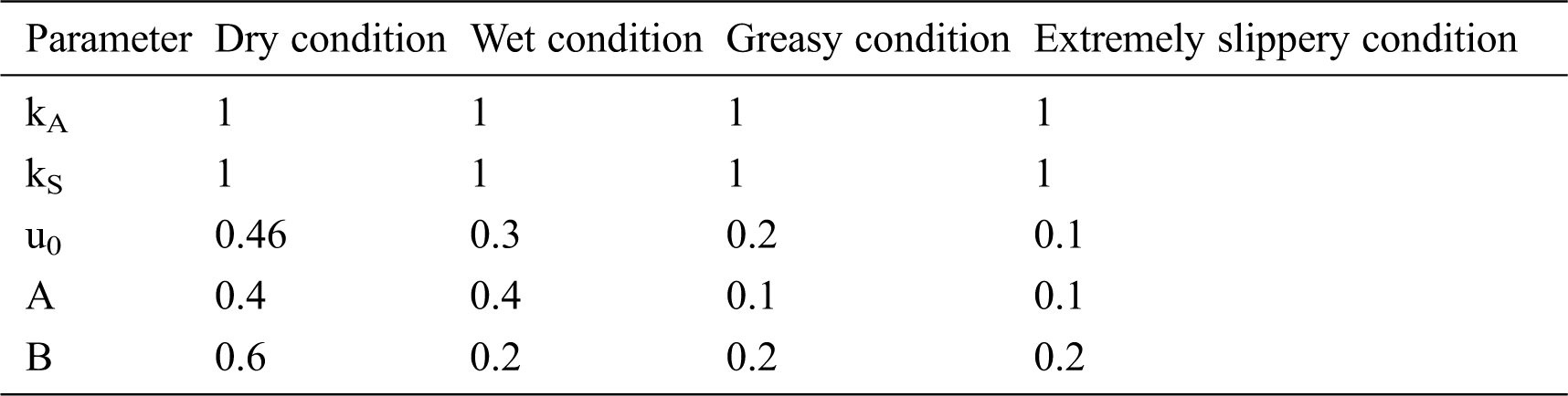
The values of Polach parameters used for tuning of the creep curves given in Tab. 1 are standard values for a railway vehicle.
Table 1: Polach parameters [11]
The slip ratio γ is the relative speed of the wheel to rail, the slip ratios of both wheels of wheelset in the longitudinal and lateral direction, and total slip ratio are presented in Eqs. (6)–(9) [18].
The total slip ratio will be:
A complete wheelset model includes all relevant motions related to wheel-rail contact forces that help to study the wheelset dynamics. The equations of motion of the railway wheelset for longitudinal, lateral, rotational, torsional, and yaw dynamics are given below [19]:
where
The centripetal force component
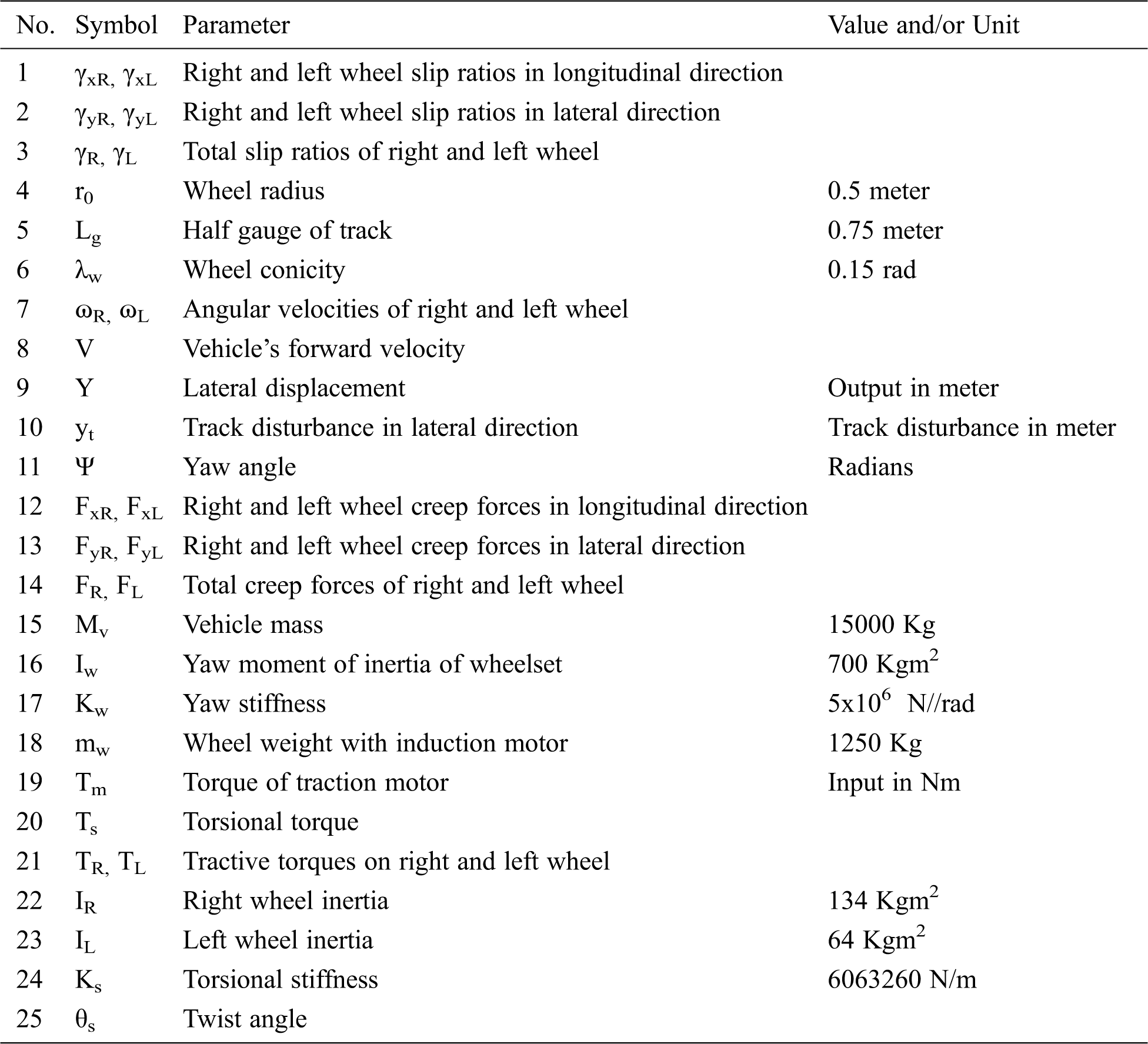
The description of the model parameters of the railway wheelset is given in Tab. 2.
Table 2: Parameters used in modeling of nonlinear wheelset dynamics
In the study of wheelset dynamics, it is important to develop and use a complete model that comprises all related motions associated with the contact forces because of powerful interactions among various motions of the wheelset play in both the longitudinal and lateral directions. Wheelsets are the element of railway vehicles that interact directly with the rail path and subsequently, the wheelset dynamics are directly affected by changing contact conditions.
A Simulink model of complete and non-linear railway wheelset, based on Eqs. (10)–(15) is developed for analyzing wheelset response. A track input yt of 5 mm step is generated to simulate wheelset dynamics to show the existence of track disturbances. The dry and wet condition creep curves of Fig. 3 are used during this simulation. The wheel slip (unwanted phenomenon) in wheelset dynamics is a consequence of the existence of low adhesion during traction and braking modes. Fig. 4 shows the tractive torque gradually increased for acceleration. Because of the slip, the equivalent linear velocity of the wheels rises surprisingly as shown in Fig. 5, affecting the mechanical parts of the rolling stock to wear down rapidly and waste of power, while the rise in vehicle velocity is much slower due to the wheel slip.
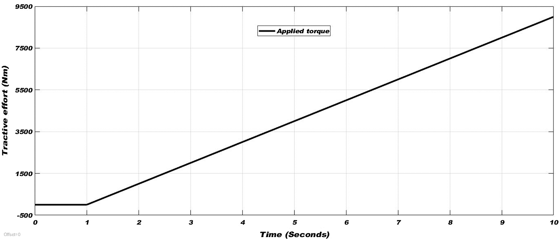
Figure 4: Applied tractive effort for acceleration
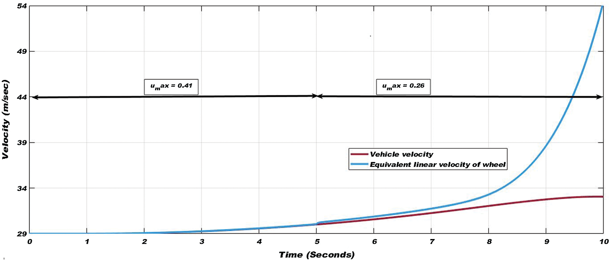
Figure 5: Vehicle velocity and equivalent linear velocity of wheel during drop of adhesion coefficient
The main objective of this study is to develop a novel model-based technique to estimate the wheelset dynamics in different contact conditions. The model-based estimation schemes using discrete Kalman filter and Bucy Kalman filter have been successfully used by many researchers for estimation of wheelset parameters [6,15,16,20,21]. However, a simple Kalman filter is not suitable for a nonlinear wheel-rail contact system. A model-based technique using EKF is therefore developed for the estimation of adhesion coefficient, slip ratio, and wheelset lateral dynamics. Because for nonlinear systems like railway wheelset, EKF is a more suitable approach. The proposed method based on the EKF algorithm is presented by using the measurements of inertial sensors mounted on the axle box of the wheelset. Fig. 6 illustrates the block diagram of EKF with the railway wheelset model. The EKF linearizes the current mean and covariance by assessing Jacobian matrices and their partial derivatives [22].
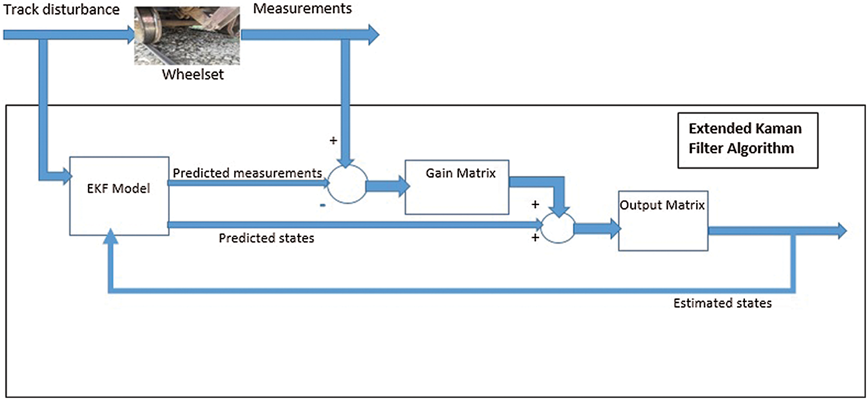
Figure 6: Block diagram of extended Kalman filter with wheelset
The nonlinear wheelset model discussed in Section 2 is used to develop the EKF algorithm. Eq. (16) is written in matrix form for designing EKF after rearranging Eqs. (11) and (12) and equating slip ratios and adhesion forces of right and left wheels.
The main objective of this study is to develop a state-of-the-art technique to detect the changes in wheel-rail contact conditions and only yaw and lateral dynamics are sufficient for detecting these changes. Therefore, longitudinal dynamics are not taken in Eq. (16).
As the Extended Kalman filter like simple KF is a 2 step predictor-corrector algorithm [23]. The equations of predictor and corrector steps are reproduced in Eqs. (17)–(21).
Equations of predictor step:
Equations of corrector step:
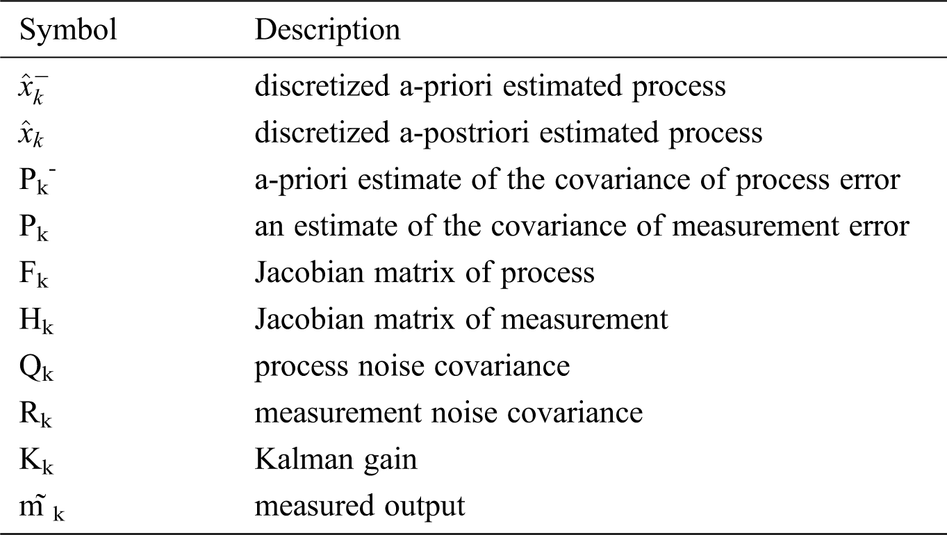
where
Table 3: Terminology of the EKF algorithm [11]
The five variables given in Eq. (22) i.e., lateral velocity (
The process variables are reproduced from Eqs. (3), (4), (9), and (16) as:
As the chosen process variables are extracted from the wheelset model and are continuous but the EKF algorithm is a discrete one, therefore equations from Eq. (23) to (27) are discretized by using the Forward Euler method [24] as:
Now the Jacobean matrix of process matrix
And the Jacobian of the measurement matrix
where:
The performance of EKF not only depends on Jacobian matrices but also the selection of Kalman gain and noise covariance contribute significantly. Kalman gain is calculated by using Eq. (19) and noise covariance
A simulation model of the proposed estimation technique shown in Fig. 6 is developed in Simulink [24]. The geometric and mechanical parameters of the wheelset given in Tab. 2 are used in the simulation. The vehicle with an initial linear velocity of 5 m/sec is operated in traction and braking modes and input of random track irregularities of ±8 mm magnitude in lateral direction shown in Fig. 7 is applied to the model for exciting lateral dynamics.
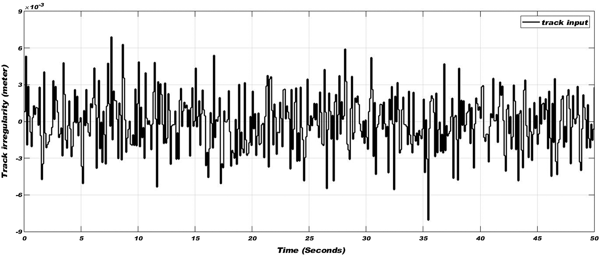
Figure 7: Track irregularities in the lateral direction
The measurement noise covariance matrix
Simulations are carried out in traction and braking modes of vehicle in five different conditions i.e., (i) Dry condition, (ii) Wet condition, (iii) Greasy condition, (iv) Extremely slippery condition, and (v) Transition from dry condition to extremely slippery condition.
The simulation in dry track conditions is carried out for 50 seconds in both accelerating and decelerating modes of a vehicle to calculate adhesion coefficient, slip ratio, and yaw rate.
In traction mode of a vehicle for 25 seconds of simulation time, tractive torque is applied to increase the linear velocity up to 30 m/sec (108 km/h), and then in braking mode of vehicle tractive torque applied in the reverse direction to reduce the velocity up to initial velocity i.e., 5 m/sec (18 km/h). In only 25 seconds, linear velocity increased from 18 km/h up to 108 km/h and in 25 seconds linear velocity decreased from 108 km/h back to the initial velocity. Both wheelset and estimator remain stable during the whole simulation time.
Applied torque and varying linear velocity are shown in Fig. 8. Adhesion coefficient, slip ratio, and yaw rate on the dry condition are shown in Fig. 9. In Fig. 9 adhesion coefficient, slip ratio, and yaw rate are perfectly estimated by EKF based estimator, however, fluctuations are developed due to change in applied torque and random track irregularities in the lateral direction. Fluctuations are also developed in linear velocity due to track irregularities but having very small magnitude, hence not visible in the graph of Fig. 8.

Figure 8: Applied torque (top) and varying forward velocity (bottom) in dry condition of wheel-rail interface
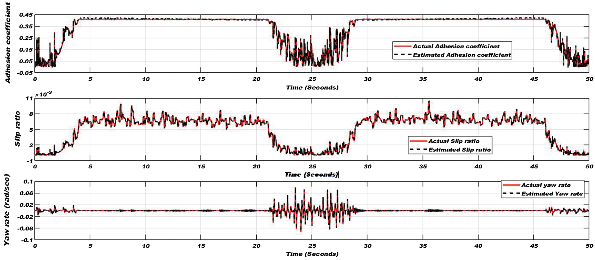
Figure 9: Adhesion coefficient (top), slip ratio (middle), and yaw rate (bottom) for the dry condition of the wheel-rail interface
The simulation in wet track conditions is carried out for 50 seconds in both traction and braking modes of the vehicle to calculate the adhesion coefficient, slip ratio, and yaw rate.
In traction mode of the vehicle for 25 seconds of simulation time, tractive torque is applied to increase the linear velocity up to 90 km/h, and then in braking mode of vehicle tractive torque applied in the reverse direction to reduce the velocity up to the initial velocity i.e., 18 km/h. Applied torque and varying forward velocity are shown in Fig. 10. Adhesion coefficient, slip ratio, and yaw rate on the wet condition are shown in Fig. 11.
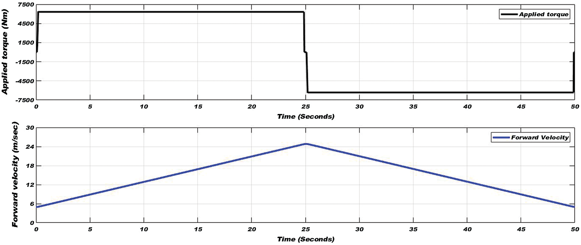
Figure 10: Applied torque (top) and varying forward velocity (bottom) in wet condition of wheel-rail interface
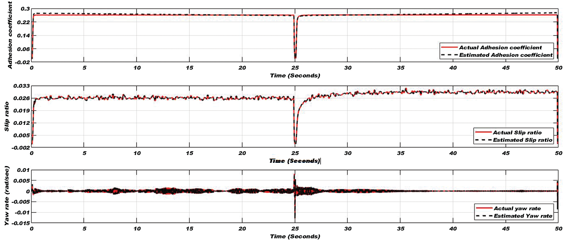
Figure 11: Adhesion coefficient (top), slip ratio (middle), and yaw rate (bottom) for the wet condition of the wheel-rail interface
The simulation in greasy track condition is carried out for 50 seconds in both traction and braking modes of the vehicle to calculate adhesion coefficient, slip ratio, and yaw rate.
In the traction mode of the vehicle for 25 seconds of simulation time, tractive torque is applied to increase the linear velocity up to 63 km/h and then in the braking mode of the vehicle tractive torque is applied in the reverse direction to reduce the velocity up to initial velocity. Fig. 12 shows the applied torque and varying forward velocity. Adhesion coefficient, slip ratio, and yaw rate on the wet condition are shown in Fig. 13.
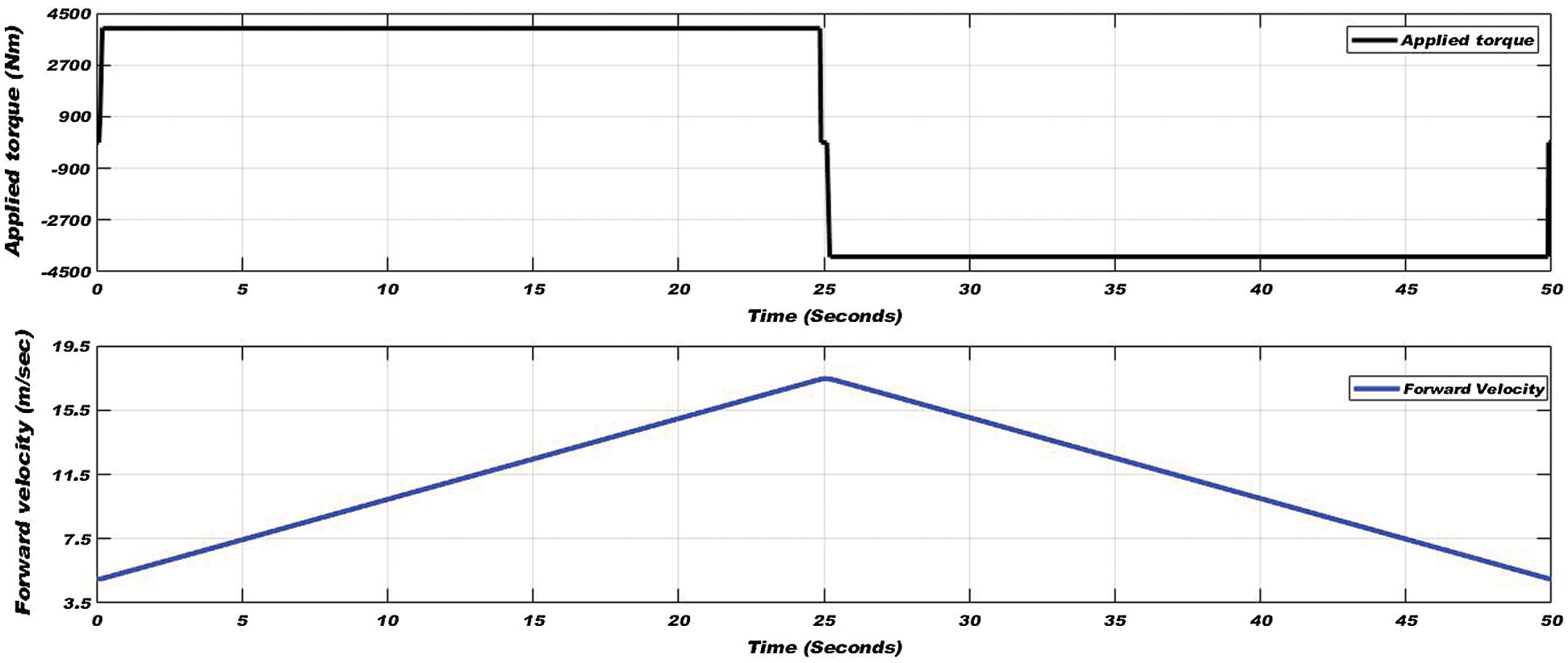
Figure 12: Applied torque (top) and varying forward velocity (bottom) in greasy condition of wheel-rail interface
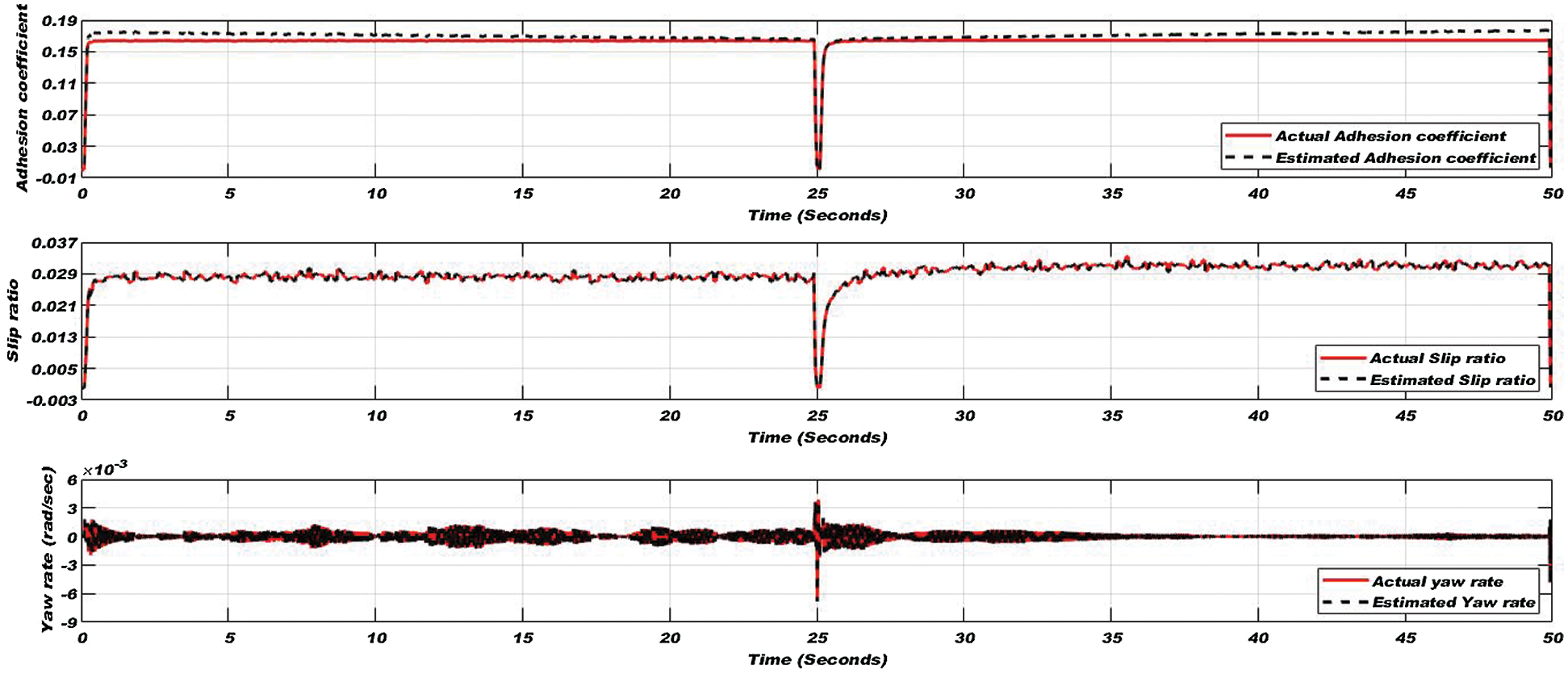
Figure 13: Adhesion coefficient (top), slip ratio (middle), and yaw rate (bottom) for the greasy condition of the wheel-rail interface
4.4 Extremely Slippery Condition
The simulation in extremely slippery track conditions is carried out for 50 seconds in both traction and braking modes of the vehicle to calculate adhesion coefficient, slip ratio, and yaw rate.
In the traction mode of the vehicle for 25 seconds of simulation time, tractive torque is applied to increase the linear velocity up to about 40 km/h, and then in braking mode of the vehicle tractive torque is applied in the reverse direction to reduce the velocity back up to 18 km/h. Applied torque and varying forward velocity are shown in Fig. 14. Adhesion coefficient, slip ratio, and yaw rate on wet conditions are shown in Fig. 15.
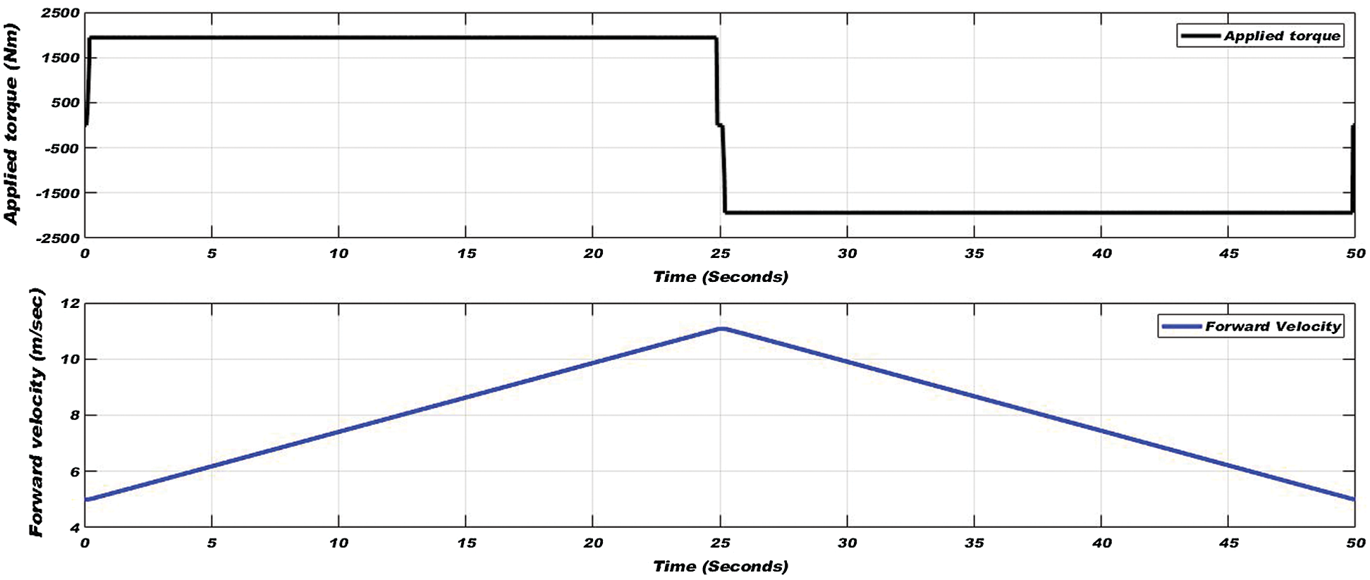
Figure 14: Applied torque (top) and varying forward velocity (bottom) in extremely slippery condition of wheel-rail interface
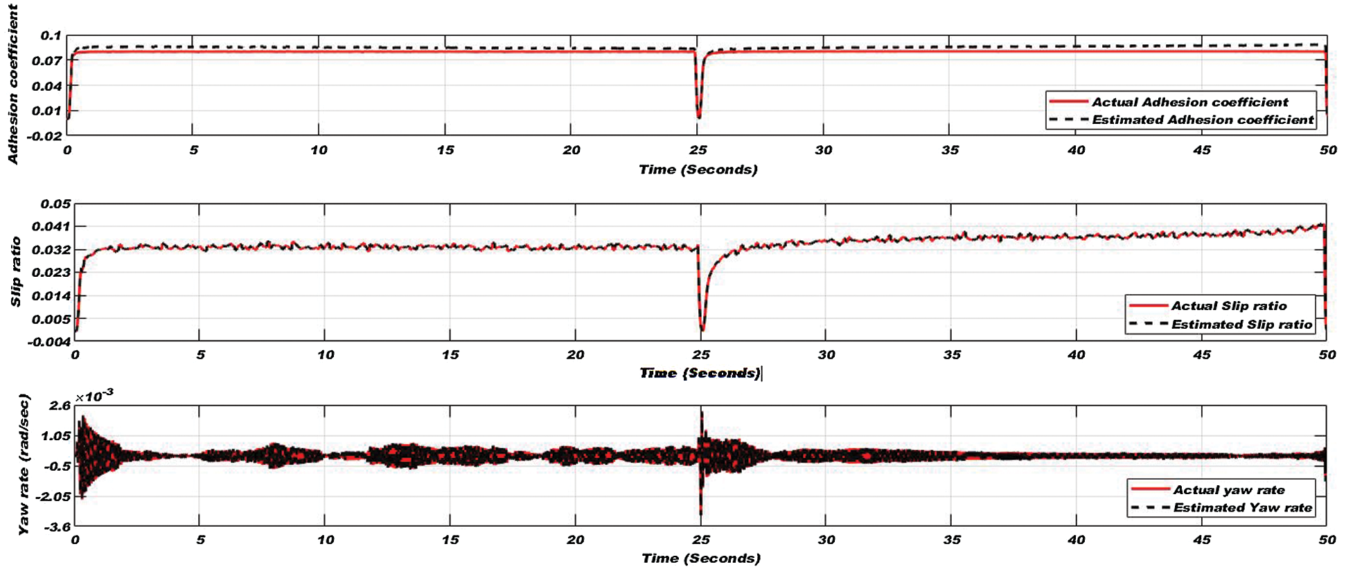
Figure 15: Adhesion coefficient (top), slip ratio (middle), and yaw rate (bottom) for the extremely slippery condition of the wheel-rail interface
4.5 Adhesion Condition is Switched from Dry to Slippery During Simulation
In this sub-section, the wheel-rail interface condition is changed during simulation from normal to extremely slippery adhesion condition in 25 seconds of simulation time and reversely adhesion condition changed from extremely slippery to dry track condition in the remaining time of the simulation. In the traction mode of the vehicle for 25 seconds of simulation time, tractive torque is applied to increase the linear velocity maximally 63 km/h, and then in the braking mode of the vehicle tractive torque is applied in the reverse direction to reduce the velocity up to initial velocity.
Further applied torque and varying linear velocity are shown in Fig. 16. Adhesion coefficient, slip ratio, and yaw rate on all conditions are illustrated in Fig. 17. In Fig. 17, the results are not linear or inconstant because of the transition of track conditions, varying linear velocity, and track disturbances in the lateral direction. Despite that, the EKF based estimator follows perfectly the results of the nonlinear wheelset.
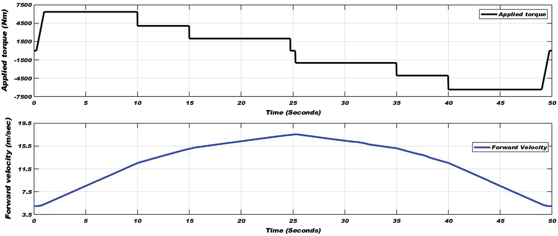
Figure 16: Applied torque (top) and varying vehicle linear velocity (bottom) in all track conditions of the wheel-rail interface

Figure 17: Adhesion coefficient (top), slip ratio (middle), and yaw rate (bottom) for all track conditions of the wheel-rail interface
As shown in Figs. 9–17 that the EKF is a valid estimation technique to estimate wheelset dynamics in both traction and braking modes. To statistically evaluate the obtained results with the proposed EKF algorithm, the absolute accuracy index (Aa) given in Eq. (37) is used [15]. The absolute accuracy index is mainly useful for measuring the disagreement of the estimation with the real signal.
The absolute accuracy indices for the estimation for all adhesion conditions are shown in Tab. 4.
Table 4: Absolute accuracy indices

It can be seen that the values of absolute accuracy indices confirm the effectiveness of the estimator. To test the performance of the proposed estimation setup, some related and recent works are chosen as the comparison techniques with equivalent system and setup. The work reported in Refs. [10,11] is only performed in normal operation mode of a railway vehicle, while the proposed technique is equally suitable in both traction and braking modes of vehicle. The work reported earlier in Refs. [10,15] shows one or two adhesion conditions but the proposed work is verified with all four adhesion conditions (dry, wet, greasy, and extremely slippery). Along with the adhesion coefficient in the proposed scheme slip ratio and yaw rate are estimated successfully, while in most of earlier work only adhesion coefficient is estimated.
The proposed EKF-based estimator shows outperformance in wheelset dynamics for dry, wet, greasy, and extremely slippery track conditions in both traction and braking modes of railway vehicles. Therefore, the proposed model can very well suit for condition monitoring of rolling stock.
The performance of railway operation mainly is affected by wheel-rail contact forces but it is not possible to measure these contact forces and interrelated dynamics directly, therefore it is necessary to estimate these wheelset dynamics through state of art technique. In this research paper, a railway wheelset model and a novel observer-based estimator are developed in Simulink/MATLAB to calculate and estimate nonlinear wheelset dynamics. The estimator based on the extended Kalman filter is used to estimate adhesion coefficient, slip ratio, and yaw rate effectively in dry, wet, greasy and extremely slippery track conditions. The functioning of the EKF algorithm is assessed by using absolute accuracy indices and compared with other relevant and recent research work. The estimator not only verified excellent performance in the normal operation of a railway vehicle on a normal track but equally depicted robustness in traction and braking modes of the vehicle in wet, oily, and extremely slippery track conditions. The validity of the estimator is also checked in the transition of adhesion conditions from dry to extremely slippery and vice-versa during the simulation. In the future, this approach will be implemented on Field Programmable Gate Arrays (FPGA) platform for real-time condition monitoring of wheelset dynamics to avoid the accidents and derailment of railway vehicle.
Acknowledgement: The authors would like to acknowledge the “NCRA Condition Monitoring Systems Lab” at Mehran University of Engineering and Technology, Jamshoro, part of the NCRA project of Higher Education Commission Pakistan, for supporting this work.
Funding Statement: This research work is fully supported by the NCRA project of Higher Education Communication Pakistan.
Conflicts of Interest: The authors declare that they have no conflicts of interest to report regarding the present study.
1. I. Hussain, “Multiple model-based real time estimation of wheel-rail contact conditions,” Ph.D. Thesis, University of Salford, Salford, 2012. [Google Scholar]
2. S. Shrestha, Q. Wu and M. Spiryagin, “Review of adhesion estimation approaches for rail vehicles,” International Journal of Rail Transportation, vol. 7, no. 2, pp. 79–102, 2019. [Google Scholar]
3. I. Hussain and T. X. Mei, “Modeling and estimation of non-linear wheel-rail contact mechanics,” in 20th Int. Conf. on System Engineering on System Engineering, Coventry, UK, pp. 219–223, 2009. [Google Scholar]
4. S. Strano and M. Terzo, “Review on model-based methods for on-board condition monitoring in railway vehicle dynamics,” Advances in Mechanical Engineering, vol. 11, no. 2, pp. 168781401982679, 2019. [Google Scholar]
5. C. Li, S. Luo, C. Cole and M. Spiryagin, “An overview: Modern techniques for railway vehicle on board health monitoring systems,” Vehicle System Dynamics, vol. 55, no. 7, pp. 1045–1070, 2017. [Google Scholar]
6. I. Hussain and T. X. Mei, “Estimation of wheel-rail contact conditions and adhesion using the multiple model approach,” Vehicle System Dynamics, vol. 51, no. 1, pp. 32–53, 2013. [Google Scholar]
7. Y. Zhao and B. Liang, “Re-adhesion control for a railway single wheelset test rig based on the behaviour of the traction motor,” Vehicle System Dynamics, vol. 51, no. 8, pp. 1173–1185, 2013. [Google Scholar]
8. Y. Zhao, B. Liang and S. Iwnicki, “Friction coefficient estimation using an unscented Kalman filter,” Vehicle System Dynamics, Vol. 52, no. 1, pp. 220–234,2014. [Google Scholar]
9. Y. Q. Sun, C. Cole and M. Spiryagin, “Monitoring vertical wheel-rail contact forces based on freight wagon inverse modelling,” Advances in Mechanical Engineering, vol. 7, no. 5, pp. 1–11, 2015. [Google Scholar]
10. S. Strano and M. Terzo, “On the real-time estimation of the wheel-rail contact force by means of a new nonlinear estimator design model,” Mechanical Systems Signal Processing, vol. 105, no. 7, pp. 391–403, 2018. [Google Scholar]
11. K. Mal, I. Hussain, B. Chowdhry and T. Memon, “Extended Kalman filter for estimation of contact forces at wheel-rail interface,” 3C Tecnol, Special Issue, Vol. 2020: pp. 279–301,2020. [Google Scholar]
12. J. Liu, L. Liu, J. He, C. Zhang and K. Zhao, “Wheel/rail adhesion state identification of heavy-haul locomotive based on particle swarm optimization and kernel extreme learning machine,” Journal of Advanced Transportation, vol. 2020, pp. 8136939, 2020. [Google Scholar]
13. S. M. Ujjan, I. H. Kalwar, B. S. Chowdhry, T. D. Memon and D. K. Soother, “Adhesion level identification in wheel-rail contact using deep neural networks,” 3C Tecnología. Glosas de innovación aplicadas a la pyme, Special Issue, vol. 2020, pp. 217–231, 2020. [Google Scholar]
14. A. Zirek, “A novel anti-slip control approach for railway vehicles with traction based on adhesion estimation with swarm intelligence,” Railway Engineering Science, vol. 28, no. 4, pp. 346–364, 2020. [Google Scholar]
15. S. Munoz, J. Ros and J. L. Escalona, “Estimation of lateral track irregularity through Kalman filtering techniques,” 2020. [Google Scholar]
16. T. Ishrat, Slip control for trains using induction motor drive. Queensland University of Technology, Australia, 2020. [Google Scholar]
17. O. Polach, “Creep forces in simulations of traction vehicles running on adhesion limit,” Wear, Vol. 258, no. 1, pp. 992–1000,2005. [Google Scholar]
18. I. Hussain, T. X. Mei and M. Mirzapour, “Real time estimation of the wheel-rail contact condtions using multi-Kalman filtering and fuzzy logic,” in Proc. 2012 UKACC Int. Conf. Control 2012, pp. 691–696, 2012. [Google Scholar]
19. I. Hussain and T. X. Mei, “Identification of the wheel-rail contact condition for traction and braking control, International Association of Vehicle System Dynamics 2011, Manchester, UK, pp. 14–19, 2014. [Google Scholar]
20. P. Hubbard, C. Ward, R. Dixon and R. Goodall, “Real time detection of low adhesion in the wheel/rail contact,” Proceedings of the Institution of Mechanical Engineers, Journal of Rail and Rapid Transit, vol. 227, no. 6, pp. 623–634, 2013. [Google Scholar]
21. P. D. Hubbard, C. Ward, R. Dixon and R. Goodall, “Verification of model-based adhesion estimation in the wheel-rail interface,” Chemical Engineering Transactions, vol. 33, pp. 757–762, 2013. [Google Scholar]
22. R. W. Ngigi, C. Pislaru, A. Ball and F. Gu, “Modern techniques for condition monitoring of railway vehicle dynamics,” Journal of Physics Conference Series, vol. 364, no. 1, pp. 1–12, 2012. [Google Scholar]
23. G. Welch and G. Bishop, An introduction to the Kalman filter. Chapel Hill, NC: Department of Computer Science, University of North Carolina at Chapel Hill, 2001. [Google Scholar]
24. P. Goddard, “Goddard consulting (modeling. simulation. data analysis. visualization),” [Online]. Available: http://www.goddardconsulting.ca/simulink-extended-kalman-filter-quarter-car.html. [Google Scholar]
 | This work is licensed under a Creative Commons Attribution 4.0 International License, which permits unrestricted use, distribution, and reproduction in any medium, provided the original work is properly cited. |