DOI:10.32604/iasc.2021.017506
| Intelligent Automation & Soft Computing DOI:10.32604/iasc.2021.017506 | |
| Article |
Thermodynamics Inspired Co-operative Self-Organization of Multiple Autonomous Vehicles
1DCS, NBC, National University of Sciences and Technology, Islambad, Pakistan
2H&BS,MCS, National University of Sciences and Technology, Islambad, Pakistan
3CSE, MCS, National University of Sciences and Technology, Islambad, Pakistan
4EE, MCS, National University of Sciences and Technology, Islamabad, Pakistan
*Corresponding Author: Ayesha Maqbool. Email: ayesha.maqbool@mcs.edu.pk
Received: 29 January 2021; Accepted: 03 March 2021
Abstract: This paper presents a co-operative, self-organisation method for Multiple Autonomous Vehicles aiming to share surveillance responsibilities. Spatial organization or formation configuration of multiple vehicles/agents’ systems is crucial for a team of agents to achieve their mission objectives. In this paper we present simple yet efficient thermodynamic inspired formation control framework. The proposed method autonomously allocates region of surveillance to each vehicle and also re-adjusts the area of their responsibilities during the mission. It provides framework for heterogeneous UAVs to scatter themselves optimally in order to provide maximum coverage of a given area. The method is inspired from a natural phenomenon of thermodynamics and presents a flexible and efficient mechanism for co-operative team formation. The idea here is to model the system as a collection of heat generating bodies and to maintain the constant system temperature across the system by introducing appropriate separation among vehicles. We also present the behavour of the algorithm with the communication constraint. The proposed method achieves special allocation objectives, even with constraint communication. It is further shown that the method can easily be adopted to arbitrary configurations according to mission requirements and team configuration. This co-operative decision making of allocating mission responsibilities by self-organising a team of vehicles adds to the overall autonomy of the Multi-vehicular system.
Keywords: Autonomous vehicles; area coverage; nature-inspired algorithms; cooperative agents; self-organization; formation control
Cooperation among Autonomous vehicles is fundamental for Multiple Autonomous Vehicles (MAV) mission. Cooperation often involves the definition of a specific formation, configuration or spatial distribution of the agents. The co-operative decision making of allocating mission responsibilities by self-organising a team of MAVs adds to the autonomy of the system. This study presents a novel system configuration for a team of co-operating agents to attain the maximum surveillance of a given region of interest autonomously. The dynamic requirement of surveillance requires regular scanning of the area for threats and other activity. It sometimes also involves perusal of threat without compromising the overall surveillance quality of region. Vehicles need to work together, maintaining a team formation in optimum manner to keep the area of interest under constant surveillance. In simple words, from any given initial position and formation an agent must be able to negotiate the surveillance responsibilities of a certain region of any given orientation with minimal human intervention. The co-operative method is presented hers in order to achieve this objective. The proposed method is inspired from phenomenon of heat transfer by moving heat sources. The idea here is to model the system as a collection of heat generating bodies and to maintain the constant system temperature across the system by introducing appropriate separation among them.
The paper is organised into three sections. The Section 1 is dedicated to the review of existing methods and systems. The new self-allocation method along with its design details is presented in the Section 2. Finally Section 3 provides an overview of simulated results and performance analysis of proposed method.
Existing solutions for automated organization follows two trends: 1. Distributed planning for resource allocation; and 2. Linearized trajectories. Distributed task allocation is the most recurring theme for the allocation of surveillance responsibilities to heterogeneous agents. One approach is to model the task allocation as an objective function to be optimized under certain constraints using Linear Programming (LP). Such objective function defines the mission goals to be met with an associated cost. Second approach of using optimization techniques over cost functions of agents/ vehicles connected in form Voronoi graphs [1–5]. As these approaches require optimization of complete system. In this propose model the individual co-operative agents collaborate in simple yet efficient manner to achieve area coverage.
The design of the objective function also depends upon the degree of impact of one agent’s actions on the decision of the others. Other factors influencing the task allocation e.g. communication, performance, system dynamics, are modelled as constraint equations. Kraus, Rizk and Plotkin presented a detailed theoretical framework for distributed task allocation for co-operative agents aiming to improve overall performance with dynamic task arrival [6–8]. It was further investigated for more flexible environments, in particular for consensus building among multiple vehicles systems by Cheng [9] and Liu [10]. Consensus building by observing mission states with poor communication is presented by Alotaibi [11]. More detailed and application orientated studies were performed in devising distributed task allocation to the rendezvouses problem for agents in the model presented by McLain [12–13]. McLain’s model generated the time critical trajectories for the team of agents enabling the entire team to arrive at a given point simultaneously. Furthermore, the constraints of safe and secure path generation through hostile region were also taken into account. Bellingham, Alighanbari, Kim and Gil’s [14–18] work emphasizes the minimum completion time in a search and destroy mission with agent/weapon to target allocation as the main objective. A more detailed model for similar Suppression of Enemy Air Defenses (SEAD) mission scenario is presented by Darrah [19]. The model for aerial surveillance using fixed wing miniature agents is developed by Beard [20]. Beard’s model optimises the co-ordination variable for mission scenarios like co-operative timing, search, fire surveillance and threat surveillance. Due to the inherent complexity of the distributed models and large state spaces LP is computationally expensive and its convergence depends on how the problem is modelled in terms of objective and constraint equations. Also factors like dual constraints and non-continuous variables make the models infeasible to solve.
Most of the work that addresses automated surveillance considers the region of allocation as a narrow linear path. Girard [21] presents a hierarchical control architecture for the border patrol by a team of agents. Here, the surveillance region is considered as a long thin border. The border is then split into sub-regions of the same size and shape by ground control. El- maliach [22] presented a detailed analysis of the frequency with which the surveillance area is visited by the team of the agents and how this is affected by adopting different strategies of overlapping and non-overlapping trajectories. The Elmaliach work on multi-robot fence patrolling mapped an open ended polygonal work area. Here the allocation of region to patrol is achieved by the spatio-temporal division of an open polygon into n subregions for n agents and assigning arbitrary subsection to each agent. A comprehensive model for surveillance using a team of small agents is presented by Kingston [23]. Because of small on-board processing power the surveillance region is converted into connected linear path at the ground control. The agents are launched into trajectories with significant time delay to maintain the trajectory separation. The agent with uniform velocity similar to the rest of the team then co-operatively finds the equal allocation by meeting its neigh- bouring agents at the end of its respective trajectory and sharing trajectory information. The application of the linearised based allocation to a circular region is presented by Casbeer [24]. Casbeer’s work addresses the surveillance of a polygonal region of forest fire. However the trajectories of the agents are still considered as linear. Similarly Sousa [25] presented the circular surveillance by agents with flight dynamics in equally spaced linear formation. In all the above mentioned methods the workspace is considered as a linear trajectory and the agents then take the task of surveillance by simply dividing the length of the entire linear workspace by the number of agents in the team.
Even though the optimization-based planning is a sophisticated and well established method for task allocation, however in the case of multiple agents and distributed objective it is computationally expensive. Even with linearized trajectories the additional requirement for converting the area of surveillance as linearized connected trajectories makes such allocation in- flexible and less adaptive for the challenges of real-time missions.
The main contribution of our proposed methods are :
1. Simple and reliable self-allocation behavior for area coverage model that can be adopted to any situation.
2. Theoretical background and proof of convergence of proposed system.
3. Simulation results along with sufficient low level constraints.
In the rest of the paper, section 2 presents the theoretical background and details of self allocation method. Section 3 simulation results of three distinct formation are presented. We conclude this paper in section 4.
The presented solution suitable for the real-time environment, is based on the idea of the distribution of vehicles (here termed as agents) at certain given length of separation between themselves. The agents maintain equidistant separation by estimating the mean reference point and surveillance radius of neighboring agent. The dynamic, flexible allocation can be achieved by modelling the system as a simple thermodynamic system. Here agents are mapped as heat sources and the mission area as a heat sink, with hotter boundaries and absolute zero at the global reference point. The formation of agents is maintained by balancing the pull towards the global reference point and the repulsion from the heat generated by the neighboring agents.
2.1 Virtual Thermodynamic Model
Consider a team of n agents where n ≥ 2 in certain region of interest for surveillance. The area dref for surveillance spans 0 to
First is the reference field, if the force of repulsion between the agents is weaker than that of the reference field, this might cause the overlapping of the individual agents surveillance areas. Conversely, if the reference field force is weaker, the agents will move away from one another due to stronger repulsive forces towards the boundaries of the region. This might also cause the agents to constantly move in circular trajectories like planetary motion and thus never settling for co-operative subregion allocation. The reference field can be seen as a force of resistance that stops the agents from getting infinitely apart under the influence of inter-agent’s repulsion. Referring back to basic Newtonian physics the resistive force is the force that an agent has to overcome before it can perform any work, i.e. displacement. An ideal frictionless system, in balance with the resistive forces is defined as :
where Fres is the resistive force, dres is the resistive distance, Fe is the effort force balancing the resistance, applied over the distance de. For a system with n agents forcing their way out of the reference field the Eq. 1 becomes:
Thus a fair design incentive for the reference force for a team of agents with individual force field
However, each agent balances itself against the opposing flux of the rest of the team and the reference field without considering its own flux, so a better choice for reference field is
In the proposed virtual setup the flux experienced by a vehicle from other vehicle can act in either direction, i.e., push it towards or away from the reference point. Thus, from the vehicle point of view there is no constant direction of net flux. At any instance the vehicle experiences thermal energy/force Ei which is the sum of the attractive and repulsive forces from the thermal sinks with lower temperatures
Now, if agent follows the Fourier law of heat transfer and moves towards the negative gradient of the temperature
where k is an appropriate constant depending upon the dynamics of agents.
where α > 0 is an appropriate positive tuning constant. Thus the new net energy can be expressed as
The system will attain steady state when there is no change in energy in any agent, i.e.,
In the proposed model the forces are mapped as modified heat sources with the monotonically decreasing function with respect to the distance,
where
Proof: Consider the agents guidance function be
As α is positive the stability of the solution depends upon the choice of functions defining the energy function. Now, in the proposed model the attractive and repulsive forces are mapped as Eq.10 with distribution σi as radius of the individual agent Ai’s surveillance region. The surveillance region with the minimum overlap is selected with respect to the location xj of the neighboring agents Aj
This makes the norm of its derivative greater than the function itself
The self-allocation method is simple in design, however, to achieve maximum coverage, the algorithmic details of the process influence the final configuration significantly. Broadly, the self-allocation method estimates two fundamental measures:

1. The mean position of the agent: The mean or the point of reference of the vehicle in the area of interest with respect to the rest of the team; and
2. The radius of surveillance: The region for repeated trajectories for the constant update of ever-changing environment.
The individual position of the agents is adjusted by moving in the appropriate direction under the influence of the different forces, and the radius of surveillance is selected depending upon the individual scanning strength and the distance between its neighboring agents. As mentioned in the section 3 the choice of mapping functions and associated factors influences the distribution and configuration of the agent’s surveillance area. The negative exponential function, Eq. 10, is selected as the navigational function for the team organization. The sink function or the workspace map is different from the individual force function with the following specifications:
•
•

2.3 System Stability and Zeroth Law of Thermodynamics
A major factor for consideration in any co-operative control is the degree of awareness an agent possesses regarding the rest of the system. In real-time mission environment sharing the complete information with
each and every agent might not be possible. of location and the radius of other agents the heat map cannot be produced. However, the proposed scheme works well even in case of incomplete information. Another advantage of using the virtual thermodynamical system is the fact that even in case of local information sharing the system still achieves the global stability by following the zeroth law of thermodynamics this aids in achieving the equilibrium in the absence of global information sharing.
Definition: The zeroth law states that if two systems are in thermal equilibrium with a third system, they are also in thermal equilibrium with each other.
By limiting the radius of each agent to just slightly larger than the observable team members, Procedure 1 step 3 maintains an even allocation of the surveillance area and observing one agent in the team helps in estimating the radius of rest.
The self-allocation method presented here addresses co-operative behavior for trajectory selection. The inputs and outputs of applied method lack low level details such as actuator controls. The output of the self-allocation method at each iteration is an immediate waypoint, pointing agent towards the appropriate direction. These waypoints may not comply with the agents motion constraints. The waypoint following is then achieved by generating feasible smooth trajectories. Trajectory smoother is employed here to generate the feasible paths by considering the time and distance constraints, e.g., heading, steering, translation velocities and acceleration constraints. The position of moving object at time t from location
In the current study, the trajectories generated in Eq.14 are continuous in terms of heading angle, angular and linear velocity limits, the angular and linear acceleration are also continuous. The difference of location on a trajectory and the discrete waypoint on the grid can be seen as the tracking error. Constraints resulting in smaller error results in lesser time delay in reaching the waypoint and larger error takes longer. Since the force maps depend upon the agent’s position, larger errors result in deflection from the desired behaviour of self-allocation scheme and results in unstable system. Care has to be taken while generating the grid of workspace such that constraints of team do not suffer from undesirable errors. For instance, a grid cell map of 10 × 10 meters area is small for an agent with velocity ranging from 0 to 100 meter/sec. Similarly, an angle steering constraint of
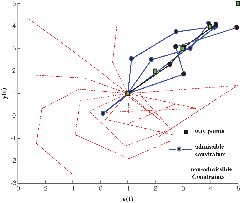
Figure 1: Range of admissible constraints for waypoint following
The following simulations present three different arrangements of team depending upon the reference point on a two dimensional workspace. The system is initialized by each agent adjusting its current radius of surveillance using algorithm radius-tuning. Then all forces are mapped by using Eq. 10. The direction of motion along each axis is calculated by adding the components of the force from the rest of the team and the reference point.
Here θ is the angle between the current agent and respective source of heat, i.e., other agent’s location or point of reference. The exponential mapping makes the magnitude of forces significantly smaller than one. The net force is then amplified to unit magnitude which translates into generating next waypoint into one of eight neighbouring cells in the grid. However, as mentioned above this waypoint may or may not be achievable due to motion constraints. A feasible trajectory is then generated towards the waypoint generated in previous step. Due to the motion constraints it may not be possible for the agent to move to the waypoint in a unit time, thus the current location of the agent is selected as its real position. It may seem that this may result in agent not following the direction of force. But the simulation results show the delay in achieving the waypoint does not affect the system reaching a stable state.
The negative exponential mapping, Eq.10, of forces becomes considerably small but not always zero. Amplification of the forces in procedure 2: Self-Allocation, step (d), may cause the stable mean position of surveillance to switch back and forth between two consecutive locations. A simple estimate of standard deviation on waypoint generated in recent iterations ensures the termination of the Self-Allocation procedure. This is however not done in the following simulations to illustrate the behaviour of the system even after the stable state is achieved. The following results show the flexibility of the proposed scheme to achieve three different team formations: 1. radial; 2. linear; and 3. with different constraint on maximum radii.
The first simulation, Fig. 2a, shows 15 agents surrounding a reference point in the centre of workspace of 500 × 500 cells. The surveillance formation can be used to guard or siege a place of interest in all directions. The gray gradient background shows the heat map of the reference field. Apart from the reference field and mutual knowledge of the fellow agents location and radius of surveillance the agents are not provided with any additional information. The constraints on motion dynamics for each agent are kept under the admissible range, i.e., steering angle is kept within ±π/
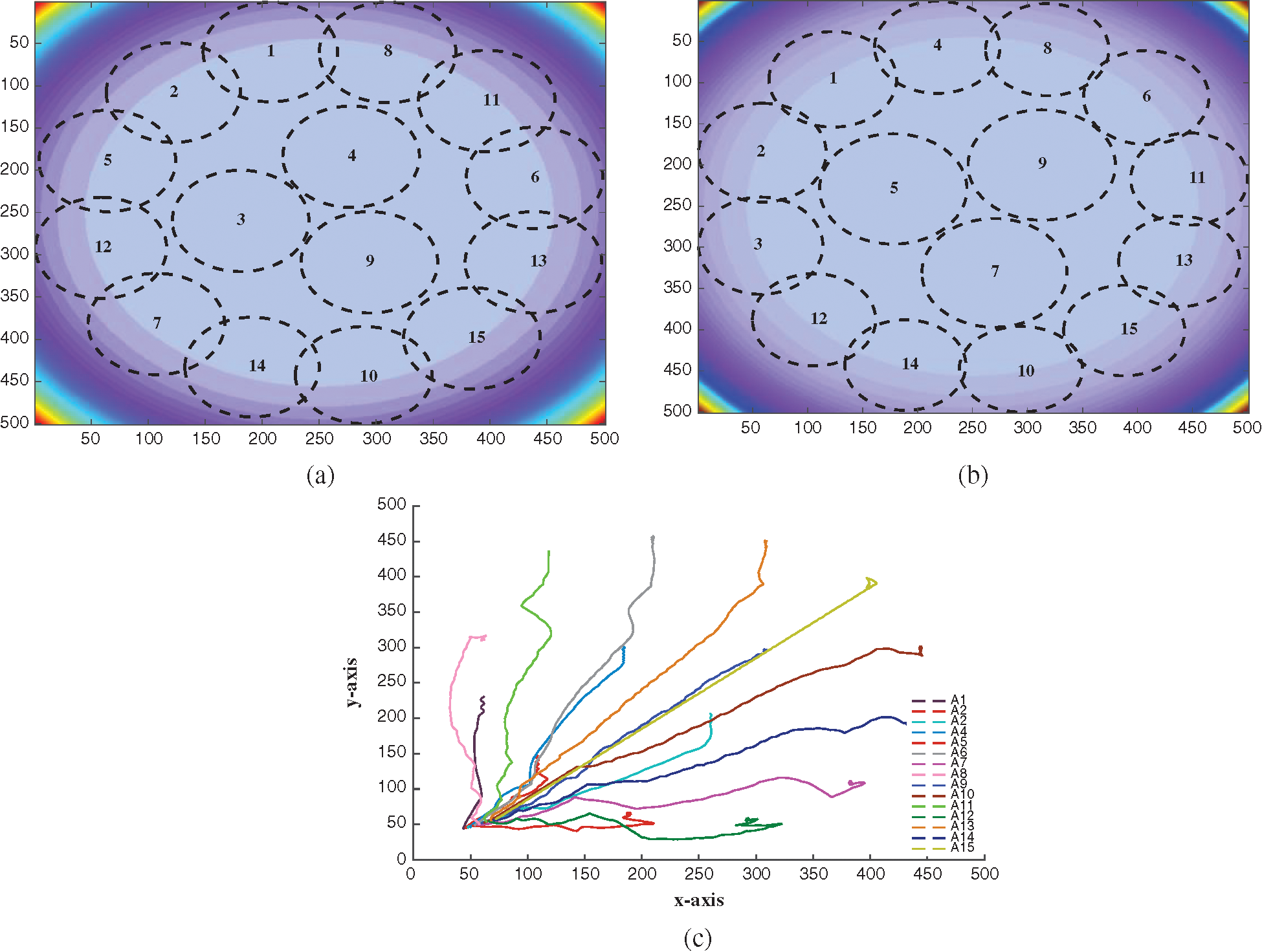
Figure 2: Radial formation trajectory and final surveillance allocation. (a) Final formation with Global awareness, (b) Final formation with Local awareness (c) Trajectories. The agents originating from a common initial location scatter themselves evenly to provide the maximum coverage of the area
The effect of local information sharing on self-allocation method are studied by simulating the communication only among the agents whose radius of surveillance collides or overlaps. The agents will exchange only their own information and do not share the details of the neighbouring agents which are within the communication range of one but not the other agent. Fig. 2c shows the final formation of the team with local awareness only. The overall final formation is same as with the full information sharing case shown in Fig. 2a. However, the positions of the agents in the formation are different. This is because the location in the final formation of individual agent is comparatively less relevant than the formation of team and objective of maximum coverage. Fig. 3a, 3b show the distance covered by individual agents in the case of global awareness and local awareness. The system is simulated for 1000 iteration in order to test the stability of the final arrangement. In both scenarios once the team achieves the stable formation it maintains that formation. Whilst, the lack of global information may cause a delay in stabilising the system the objective of maximum coverage is not compromised. The Fig. 3b shows similar behaviour to that of Fig. 3a. After 200 in Fig. 3b iteration the system starts to divert from Fig. 3a. This divergence becomes more prominent as the agents grow apart and the local information becomes limited to few neighbouring team members. However, system achieves the stable state eventually even when in final state not a single agent possesses the global information of state of the rest of team. Thus the system follows second law of thermodynamics. Even from a comparatively erratic behaviour due to lack of global awareness the system stabilises as each agent reaches to stable state in comparison to its neighbours and achieves global stability by being in equilibrium with the neighbouring agents of the neighbouring agents. The radius of area of surveillance is also affected by the communication constraints. In Fig. 2a agents the inner circle agents 3,4,9 have lesser overlapsping boundaries as compared to agent 5,9,7 in Fig. 2c. The reason for this slight difference is the condition of selecting the radius of surveillance with respect to the neighbours in radius tuning algorithm. Therefore in case of complete awareness entire team have same radii, on the other hand due to lack of communication between the agents agents 5,9,7 have slightly bigger radii. Fig. 4a and 4b show the change in radii of team in full awareness in comparison to the local awareness only. The inner agents 5,9,6 end with slightly bigger stable radii, which in turn results in better coverage of the surveillance space. But it can be seen in the final formation in both cases that difference of radii allocation does not effect the coverage of surveillance formation.
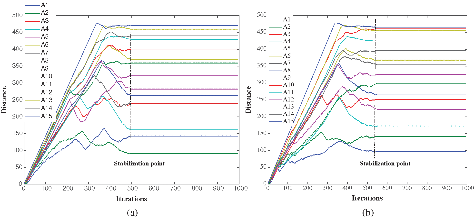
Figure 3: Formation A: Effect of communication on runtime and individual distance. (a) Global Awareness (b) Local Awareness

Figure 4: Formation A: Effect of communication on radii of surveillance. (a) Global Awareness (b) Local Awareness
The simulation shows (Fig. 5a) six agents in linear formation in the workspace of 200 × 40 dimension. Here the reference field originates from the centre, i.e., from (100,20). The dynamics of agents are kept the same as in the previous example. In order to achieve the linear formation parallel to x-axis the agents only need to tune their location along x-axis. As all agents have to align themselves in the same position along y-axis, the inter agent location of the team along y axis is considered irrelevant. Here the force along y-axis is mapped only using the force of reference field and force of rest of the agents are ignored.
Fig. 5b shows the individual tracks of the agent. In this case the agents do not start from the same location but still similar final formation is achieved with full awareness of the system as well as with the lack of global awareness. Fig. 6a, 6bshow 1000 iterations the distance covered by each agent simulated with both

Figure 5: Formation B: Linear Formation. (a) Linear formation (b) agent’s track: The agents take same path in both global and local information sharing

Figure 6: Linear Formation runtime and distance travelled. (a) Stabilization with global awareness (b) Stabilization with local awareness
full information sharing and with agent being aware of only at most two other agents. It can be seen that in both cases the system stabilises fairly early and the effect of lack of global information is minimal.
3.3 Formation C: Varying Radii
The proposed method can also be employed for team of agents with varying capabilities. Fig. 7 shows the final formation of the three pairs of agents with constraints on maximum radius of 20, 30, 40 respectively. Fig. 7 also shows the constant roaming of agents in repetitive surveillance trajectories once the agent achieves a stable mean position. The waypoints of roaming trajectories are generated when the standard deviation of mean position reduces to zero. The different radii do not affect the performance of the proposed method and maximum surveillance of the given region is achieved without any additional changes.

Figure 7: Allocation with varying radius of surveillance
The proposed system presents a new method of self-allocation, self-formation for a team of agents. The proposed method is more autonomous than the linearised approach and more flexible than the task allocation method. It does not rely on preprocessed trajectories and does not suffer from poten- tial conflicting constraints. It requires lesser data to be exchanged in order to achieve its objectives and produces similar results even when lacking the information. It not only optimally achieves the objectives of even allocation but also performs well under communication constraints.
Funding Statement: The authors received no specific funding for this study.
Conflicts of Interest: The authors declare that they have no conflicts of interest to report regarding the present study.
1. Y. Kantaros, M. Thanou and A. Tzes, “Distributed coverage control for concave areas by a heterogeneous robot-swarm with visibility sensing constraints,” Automatica, vol. 53, no. 11, pp. 195–207, 2015. [Google Scholar]
2. O. Arslan and D. E. Koditschek, “Voronoi-based coverage control of heterogeneous disk-shaped robots,” IEEE Int. Conf. on Robotics and Automation (ICRA), pp. 4259–4266, 2016. [Google Scholar]
3. T. Jing, W. Wang, T. Wang, X. Li and X. Zhou, “Dynamic control scheme of multiswarm persistent surveillance in a changing environment,” Computational Intelligence and Neuroscience, vol. 2019, pp. 1–11, 2019. [Google Scholar]
4. H. Hildmann, E. Kovacs, F. Saffre and A. Isakovic, “Nature-inspired drone swarming for real-time aerial data-collection under dynamic operational constraints,” Drones, vol. 3, no. 3, pp. 71–96, 2019. [Google Scholar]
5. F. Ye, J. Chen, Y. Tian and T. Jiang, “Cooperative task assignment of a heterogeneous multi-UAV system using an adaptive genetic algorithm,” Electronics, vol. 9, no. 4, pp. 687–701, 2020. [Google Scholar]
6. S. Kraus and T. Plotkin, “Algorithms of distributed task allocation for co-operative agents,” Theoretical Computer Science, vol. 242, no. 1–2, pp. 1–27, 2000. [Google Scholar]
7. Y. Rizk, M. Awad and E. W. Tunstel, “Cooperative heterogeneous multi-robot systems: A survey,” ACM Computing Surveys (CSUR), vol. 52, no. 2, pp. 1–31, 2019. [Google Scholar]
8. Y. Kantaros and M. M. Zavlanos, “Distributed communication-aware coverage control by mobile sensor networks,” Automatica, vol. 63, no. 4, pp. 209–220, 2016. [Google Scholar]
9. Y. Cheng, L. Shi, J. Shao and W. Zheng, “Seeking tracking consensus for general linear multiagent systems with fixed and switching signed networks,” IEEE Trans. on Cybernetics, 2020. [Google Scholar]
10. X. Liu, Z. Kexue and X. Wei-Chau, “Consensus seeking in multi-agent systems via hybrid protocols with impulse delays,” Nonlinear Analysis: Hybrid Systems, vol. 25, no. 6, pp. 90–98, 2017. [Google Scholar]
11. E. Alotaibi, T. Ebtehal, A. S. Saleh and K. Anis, “Lsar: Multi-UAV collaboration for search and rescue missions,” IEEE Access, vol. 7, pp. 55817–55832, 2019. [Google Scholar]
12. T. W. McLain, P. R. Chandler and M. Pachter, “A decomposition strategy for optimal coordination of unmanned air vehicles,” Proc. of the 2000 American Control Conf., vol. 1, pp. 369–373, 2000. [Google Scholar]
13. T. W. McLain, P. R. Chandler, S. Rasmussen and M. Pachter, “Cooperative control of UAV rendezvous,” Proc. of the 2001 American Control Conf., vol. 3, pp. 2309–2314, 2001. [Google Scholar]
14. J. S. Bellingham, M. Tillerson, M. Alighanbari and J. P. How, “Cooperative path planning for multiple UAVs in dynamic and uncertain environments,” Proc. of the 41st IEEE Conf. on Decision and Control, vol. 3, pp. 2816–2822, 2002. [Google Scholar]
15. Z. Yun, Y. Peiyang, Z. Jieyong and W. A. N. Lujun, “Formation and adjustment of manned/unmanned combat aerial vehicle cooperative engagement system,” Journal of Systems Engineering and Electronics, vol. 29, no. 1, pp. 116–133, 2018. [Google Scholar]
16. L and L. Babel, “Babel Coordinated target assignment and UAV path planning with timing constraints,” Journal of Intelligent and Robotic Systems, vol. 94, no. 3, pp. 857–869, 2019. [Google Scholar]
17. Y. Kim, D. W. Gu and I. Postlethwaite, “Real-time optimal mission scheduling and flight path selection,” IEEE Trans. on Automatic Control, vol. 52, no. 6, pp. 1119–1123, 2007. [Google Scholar]
18. A. Gil, K. Passino, S. Ganapathy and A. Sparks, “Cooperative task scheduling for networked uninhabited air vehicles,” IEEE Trans. on Aerospace and Electronic Systems, vol. 44, no. 2, pp. 561–581, 2008. [Google Scholar]
19. M. Darrah, “Multiple UAV task allocation for an electronic warfare mission comparing genetic algorithms and simulated annealing, Technical Report, DTIC Online Information for the Defense Community Document, 2006. [Google Scholar]
20. R. W. Beard, T. W. McLain, D. B. Nelson, D. Kingston and D. Johanson, “Decentralized cooperative aerial surveillance using fixed-wing miniature UAVs,” Proc. of the IEEE Conf. on Decision and Control, vol. 94, no. 7, pp. 1306–1324, 2006. [Google Scholar]
21. A. Girard, A. Howell and J. Hedrick, “Border patrol and surveillance missions using multiple unmanned air vehicles,” in 43rd IEEE Conf. on Decision and Control (CDC). Vol. 1, pp. 620–625, 2004. [Google Scholar]
22. Y. Elmaliach, N. Agmon and G. Kaminka, “Multi-robot area patrol under frequency constraints,” Annals of Mathematics and Artificial Intelligence, vol. 57, pp. 293–320, 2009. [Google Scholar]
23. D. Kingston, R. Beard and R. Holt, “Decentralized perimeter surveillance using a team of UAVs,” IEEE Trans. on Robotics, vol. 24, no. 6, pp. 1394–1404, 2008. [Google Scholar]
24. D. Casbeer, D. Kingston, R. Beard and T. McLain, “Cooperative forest fire surveillance using a team of small unmanned air vehicles,” Int. Journal of Systems Science, vol. 37, no. 6, pp. 351–360, 2006. [Google Scholar]
25. J. de Sousa and A. Girard, “Dynamic teams of networked vehicle systems,” IEEE Portuguese Conf. on Artificial Intelligence, pp. 230–235, 2005. [Google Scholar]
 | This work is licensed under a Creative Commons Attribution 4.0 International License, which permits unrestricted use, distribution, and reproduction in any medium, provided the original work is properly cited. |