DOI:10.32604/iasc.2021.015708
| Intelligent Automation & Soft Computing DOI:10.32604/iasc.2021.015708 | |
| Article |
Automatic PSO Based Path Generation Technique for Data Flow Coverage
1College of Computers and Information Technology, Taif University,PO BOX 11099, Taif, 21944,Saudi Arabia
2Dept. of Mathematics and Computer Science, Faculty of Science, Beni-Suef University,Beni-Suef, 62521,Egypt
3Dept. of Computer Science, Faculty of Science, Minia University,Minia,Egypt
4Faculty of Computing and IT, Northern Border University,Saudi Arabia
*Corresponding Author: Ahmed S. Ghiduk. Email: asaghiduk@tu.edu.sa
Received: 03 December 2020; Accepted: 06 March 2021
Abstract: Path-based testing involves two main steps: 1) finding all paths throughout the code under test; 2) creating a test suite to cover these paths. Unfortunately, covering all paths in the code under test is impossible. Path-based testing could be achieved by targeting a subset of all feasible paths that satisfy a given testing criterion. Then, a test suite is created to execute this paths subset. Generating those paths is a key problem in path testing. In this paper, a new path testing technique is presented. This technique employs Particle Swarm Optimization (PSO) for generating a set of paths to satisfy the all-uses criterion. To construct such paths for programs with loops, the proposed technique applies the ZOT-criterion. This criterion selects paths that traverse loops 0, 1, and 2 times. The proposed technique utilizes the decision-decision graph of the program under test to represent the position vector of the particle. To evaluate the efficiency of the presented technique, an empirical study has been conducted, which included 15 C# programs. In this study, the proposed technique has been compared with a genetic algorithm (GA)-based one. The results showed that the PSO required 199 generations, while the GA required 349 generations, to satisfy all def-use paths of all programs. In addition, the proposed technique required a smaller number of paths than the GA-based one.
Keywords: Data flow testing; genetic algorithm; path testing; particle swarm optimization
Path testing requires executing each path in the code under test at least once. However, executing all paths is impossible as a program with loops may include an infinite number of paths. This issue may be addressed by using a subset of all executable paths that satisfy a given path selection criterion. Finding this subset of paths is a significant challenge in path testing.
Scholars presented many path-generation approaches. Bertolino and Marre [1] presented a technique constructing a set of paths that satisfy all arcs of the tested program control-flow graph. Other studies have concentrated on generating the set of basis paths (i.e., the class of all linearly independent paths) [2–8]. The number of the basis paths can be estimated by the Cyclomatic Complexity [2] of the code under test.
Particle Swarm Optimization (PSO) is an evolutionary search-based technique proposed in 1995 by Kennedy and Eberhart [9]. PSO simulates the behavior of animal species that live in large colonies such as bird flocks and fish schools [9,10]. PSO was used for the first time to solve the traveling salesman problem [11]. PSO [12–17], Adaptive Random [18], and Genetic Algorithms (GAs) [19–21] have been applied in many software testing activities such as test data generation. GAs [8,22–25], Tabu Search Algorithm [23,26–31], State-based meta-heuristic Algorithm [32], and Clustering and Code Change Algorithm [33–35], have been used to find test paths. According to the best of our knowledge, there is not any scientific work that applies PSO in test paths generation.
This paper introduces a path testing approach that utilizes PSO for finding the paths required to cover the all-uses criterion proposed by Rapps and Weyuker [36]. The presented technique accomplishes this process by creating new paths using the formerly promising ones. The approach uses a criterion called ZOT-criterion to construct paths for programs with loops [37]. This criterion targets paths that traverse loops 0, 1, and 2 times. The approach also uses the edges of the decision-decision graph (dd-graph) of the code under test for encoding the position vector. The approach encodes the position vector of any particle as an integer array. The paper presented an experimental comparison between the proposed approach and a GA-based one. This comparison considered two main factors: 1) the number of generations required to find a path-cover for all def-use criterion, and 2) the size of this path-cover.
The rest of this paper is organized as follows. Section 2 presents a description of data-flow concepts. Section 3 discusses the basic PSO algorithm. Section 4 presents the proposed POS algorithm. Section 5 introduces the proposed PSO-based approach. Section 6 discusses the findings of the experimental study carried out to evaluate the proposed technique. Finally, Section 7 summarizes this work and gives some points for future work.
Data-flow concepts consider the relations between the definitions (def) and references (use) of the variables in the program under test. Data-flow methods employ the control-flow graph of the program to find the relations between defs and uses.
The control flow of a program may be represented by a directed graph, named the control-flow graph (CFG). A CFG consists of a group of vertices and a group of arcs (edges). Each vertex represents one statement or a group of consecutive statements. Each arc represents a potential transfer of control flow between vertices. A path in a CFG is a finite sequence of vertices linked by arcs. A complete path is a path that starts at the entry vertex and ends at the exit vertex of the CFG. A path is called a def-clear path for a variable if it does not include a new definition for that variable.
The proposed approach uses a reduced form of the CFG, named a decision-decision graph (dd-graph). In a dd-graph, every arc is a decision-to-decision path (dd-path). Fig. 3 shows the dd-graph that corresponds to the CFG (shown in Fig. 2) of the C# code given in Fig. 1. Tab. 1 presents the dd-paths, which match the arcs of the dd-graph shown in Fig. 3.
Rapps and Weyuker [32] presented a set of dataflow testing criteria, such as the all-uses criterion. All-uses criterion requires the execution of a def-clear path from each def of a variable to each use of that variable. The required def-clear paths to fulfil the all-uses criterion are named def-use paths. Def-use paths are built using the def-use associations of program variables by the method presented by Girgis [38]. Tab. 2 presents all def-use associations of the C# code given in Fig. 1 and their killing nodes. Killing nodes are those nodes that must not be included in a def-use path of a variable (i.e., nodes that contain other definitions for that variable).
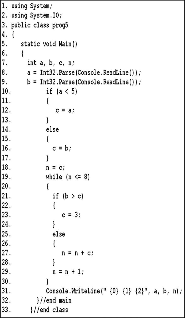
Figure 1: C# example code

Figure 2: CFG of the main class of the C# example code
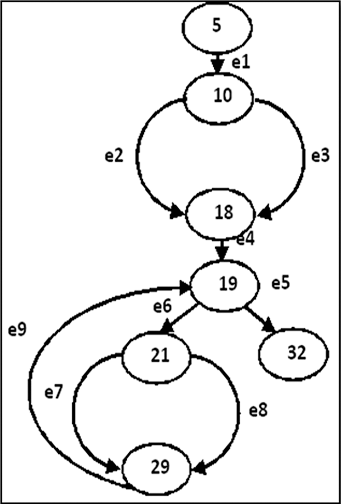
Figure 3: dd-graph for the main class of the example code
PSO is a search-based optimization algorithm that is inspired by the motion and intelligence of flocks of animals. PSO employs the concept of social interaction to solve the given problem. A comprehensive survey of PSO applications was presented by Sengupta et al. [39]. PSO concepts are based on the motion of a set of particles in the search domain to find the best solution. Every particle is handled as a single node in an N-dimensional domain. Every particle regulates its “flying” based on its personal “flying experience” and the “flying experience” of the others.
Each particle has a fitness value estimated using a fitness function and velocities. PSO has two changeable variables:
1. pbest (personal best): saves the coordinates of the best position of the current particle in the solution domain. This position corresponds to the greatest solution achieved up to now by the particle.
2. gbest (global best): is the greatest value achieved up to now by any particle inside the neighborhood of the current particle.
Every particle attempts to adjust its position based on four factors: 1) the present place; 2) the present velocity; 3) the distance from the present place to pbest; and 4) the distance between the present place and gbest. The PSO steps are demonstrated below.
At first, the initial position and the initial velocity of each particle are randomly assigned. Then, the fitness function of each particle is calculated and compared to the fitness value of the pbest location. If the present location has a fitness value greater than the pbest, then the present location becomes the new pbest. The greatest value of all pbests becomes the gbest. The position and velocity of each particle in the swarm are modified based on this gbest. The overall procedure is repeated until a specific number of generations (mGens) is reached.
Table 1: The edges of the dd-graph shown in Fig. 2 and the corresponding dd-paths

Table 2: List of def-use pairs and killing nodes of the example program, (−1 means no killing nodes)

The outcome of this algorithm is the global best value. The fitness function of the algorithm depends on the type of the application of the PSO. The updates of the position and velocity of each particle are calculated by the following equations [40]:
where:
1.
2. K: constriction factor that is required to guarantee the convergence of the PSO [41].
3. c1, c2 : learning factors.
4. r1,r2 : uniformly distributed random number between 0 and 1.
5.
6. pbesti :pbest of particlei .
7. gbest:gbest of the group.
Eq. (1) is applied to update the velocity of the particles. In addition,Eq. (2) is applied to update the position of the particles.
The PSO specifications can be:
1. The learning factors c1 and c2 are values in the interval from 0 to 4. Where the best values of c1 and c2 are determined empirically. The proposed algorithm was executed 20 times on each subject program and the best values of c1 and c2 were determined.
2. The number of particles is based on the PSO application. Commonly, the number of particles is in the range from 20 to 40;
3. The fitness function of the PSO is very related to the representation of the given problem.
The proposed PSO-based approach targets the automatic generation of test paths. The technique looks for the paths that fulfill the all-uses criterion. If the program under test contains loops, the proposed technique creates a subset of those paths that satisfies the ZOT-criterion.
In the proposed PSO algorithm, the position vector of a particle symbolizes the edges of a path through the program dd-graph. The length, L, of any position vector can be calculated using the formula L = n + 2 + p, where n + 2 is the number of edges in the dd-graph plus two more edges representing the entry and exit ones. In addition, p is the number of edges enclosed in the loops, which are included twice. This representation guarantees that the paths created for any program with loops satisfy the ZOT-criterion. For instance, the basic edges of the dd-graph of the C# code given in Fig. 3 are
where edges
The proposed algorithm employs two different forms for the position vector. The first form is a binary form called bit position vector. The second form is an integer form called actual position vector. Through any bit position vector, the digit
Suppose a particle has the following bit position vector:
The position vectors of the particles represent a group of paths. These vectors are symbolized by two forms of length L: bit position vector and actual position vector. To form the initial population, the proposed technique randomly creates PS bit arrays of length L, where PS is the population size. In each vector, the first, second, and last cells are filled with 1’s to represent the entry, first, and exit edges that have to be exist in all paths. The proper value of the size of the population is empirically determined. The algorithm creates for every produced binary position vector the corresponding actual position vector. All paths in the produced population must satisfy the connectivity rule (i.e., composed of a series of connected edges). The algorithm discards any disconnected path and generates another one to replace it. Also, the algorithm randomly creates PS velocity vectors for the initial position population. The values of every velocity vector are integers randomly selected from the interval [0, L-1]. The values of the first, second, and last cells are 0, 0, and L, respectively. This configuration guarantees that the update process of the actual position vector produces a path that contains the entry, first, and exit edges.
4.3 Position and Velocity Vectors Updating
PSO algorithms update the position and velocity of a particle using Eqs. (1) and (2). These equations can only be applied in continuous optimization problems. In the proposed approach, updating the velocity and position are accomplished using the actual position and velocity vectors, which are encoded as integer sequences, rather than real-number vectors. So, the current forms of addition and subtraction in Eqs. (1) and (2) are not applicable to the problem of path generation. Therefore, in the proposed algorithm, addition and subtraction operations in the basic velocity and position updating equations are modified to work with the path generation problem.
The presented technique utilizes two operators: the first is subtracting-two-positions operator and the second is adding-position-to-velocity operator. The two operators are applied to the members of the current population to form a new population.
Subtracting-two-positions operator: The equation of updating the velocity vector (Eq. (1)) contains two terms for subtracting positions. We suggested the following definition (Eq. (4)) for this operator.
where
Adding-position-to-velocity operator: The equation of updating the position vector (Eq. (2)) adds the new velocity to the old position. We suggested the following definition (Eq. (5)) for this operator.
where
If the updated position vector is disconnected (i.e., it contains two consecutive edges that are not adjacent edges in the dd-graph), the algorithm tries to make it connected, by adding and/or removing one or more edges to/from it. The number of edges to be added or removed to connect the disconnected part depends on the length of the sub-path between the two disconnected edges and according to their positions in the dd-graph. If no sub-path can be added to fill the gap in the disconnected path, the algorithm tries to remove some edges to connect that path. Otherwise, the algorithm discards the disconnected vector and replaces it with the original position vector. Finding a sub-path to be added or removed to fill the gap in a disconnected path is a trial-and-error process. We used the algorithm given below (Algorithm Connect) to fill the gap between any two edges in the vector.

It should be noted that the resultant position vector p’ may include a set of repeated values. If the repeated values are not indices of edges of a loop, these values are replaced by −1. The cells of the vector that represent indices for edges of a loop are allowed to be repeated only once. Therefore, an index for an edge in a loop can exist twice in the resulting position vector: the first existence is the original index and the second is the copy. To illustrate this rule, assume that p’ is 0, 1, 5, 6, 6, 12, 4, 12, 13, 3, 3, 12, 13, 8, 14. Now, the rule is applied to the resultant position p’ as follows:
1. The value 6 is an index of an edge in a loop. This edge is repeated twice. So, the first existence is not changed, while the second existence is replaced by the index of its copy, 10.
2. The value 12 is the index of the copy of the edge 8 in a loop. This edge is repeated three times, and the value 8 already exists as well. This means that this edge has 4 occurrences. The last two occurrences are replaced by the value −1. The other two occurrences are kept with changing the value of the first occurrence to the index of the original loop edge, 8.
3. The value 13 is the index of the copy of the edge 9 in a loop. This edge is repeated twice. These two edges are kept with changing the value of the first occurrence to the index of the original loop edge, 9.
4. The value 3 is not the index of a loop edge. This edge is repeated twice. The second occurrence is replaced by the value −1.
5. The values 0, 1, 4, and 14 are kept without change.
The resultant actual position becomes:
The final form of the updated actual position vector is obtained by sorting the positive values and keeping −1’s at the end, as follows:
The algorithm assesses every path (p) using the ratio of the number of the def-use paths, which it covers, to the total number of def-use paths in the program. A def-use (du) is covered if there is a path contains a sub-path that begins with the def-node (d) and finishes with the use-node (u) and that path doesn’t contain any killing node for that def-use. The fitness value fitness(Pi) of a particle Pi (i = 1, …, PS) is computed using the following formula [42,43]:
The main modules of the system that implements the presented path generation technique are described below.
The system is written using C# programing language. It contains the following modules:
1. Analysis module.
2. Path generation module.
These modules are discussed in more detail in the following subsections. Fig. 4 presents the pseudo-code of the proposed system. This system applies the proposed PSO algorithm given in Section 4.
This module accepts as input the source code P to be tested, analyses it, and produces the following outputs:
1. A report that involves the details of the components of P.
2. The CFG of P.
3. The set of all def-use pairs for each variable in P.
4. The dd-graph of the CFG of P.
For instance, the analysis module generates for the C# code given in Fig. 1: 1) the CFG given in Fig. 2, 2) the dd-graph given in Fig. 3, 3) dd-edges and its corresponding nodes given in Tab. 1, and 4) all def-use pairs given in Tab. 2.
This module applies the PSO algorithm given in Section 4 to create paths to cover all def-use pairs of the code under test. The inputs of that module are:
1. Set of def-use paths (to be covered).
2. The dd-graph size (number of edges).
3. The population size (PS).
4. Maximum number of generations (mGens).
5. Learning factors (c1 and c2).
The outputs of this module are:
1. List of paths, which satisfy the def-use criterion of the given code. It should be noted that the algorithm may fail to find paths to cover some def-use paths when these paths are infeasible, i.e., no executable path can be found to cover these paths.
2. A report presents the constructed path(s) and the satisfied def-use pairs and the set of unsatisfied def-use pairs, if any.
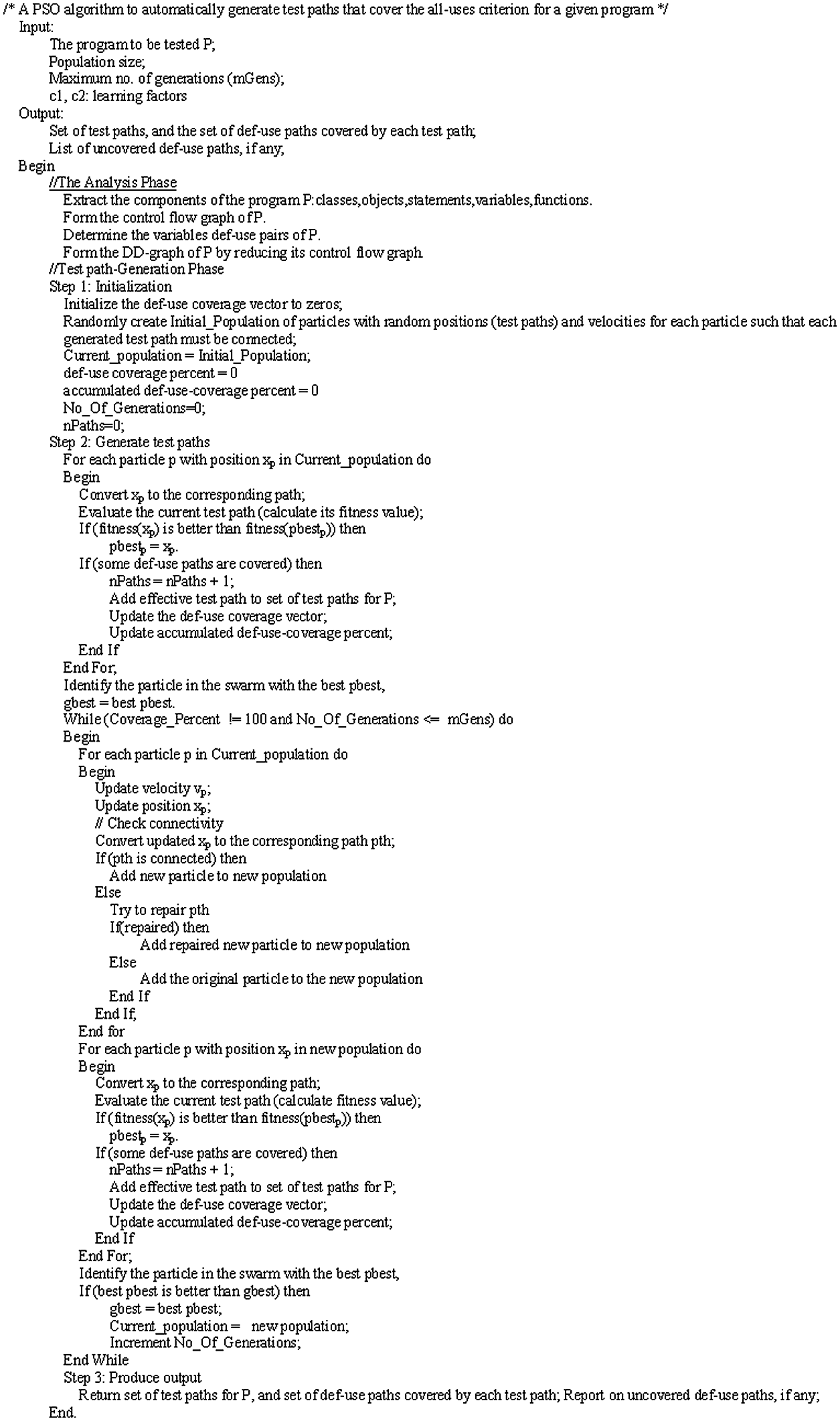
Figure 4: The whole pseudo-code of the proposed system
In the basic PSO algorithm, the population is evolved until one of its members represents the solution of the given problem. In the test path generation problem, this would correspond to one path achieving the coverage of all def-use paths of the program. Whilst this feasible for some programs, the majority of programs cannot be covered by just one test path – it might take many test paths to cover all def-use paths. Therefore, in the proposed PSO algorithm, the population evolves until a combined subset of the population satisfies the def-use criterion. This is done by recording which def-use paths of the program each member has covered and halting the evolution when a set of members has traversed the entire def-use paths of program, if possible. The solution is this set.
Figs. 5a and 5b present a part of the report generated by the path generation module after applying it to the C# program given in Fig. 1. The report illustrates that the technique created 8 paths to cover 100% of all def-use pairs given in Tab. 2. Fig. 6 presents the report generated by the technique for these 8 paths that needed 9 iterations to be covered. The list of paths that were created by the presented technique may be input to a data generation system for creating a number of inputs, which satisfy the data-flow paths testing.
This section describes the experimental study that was carried out to assess the efficiency of the proposed technique. In this study, we compared the proposed technique with the GA-based path generation system presented by Girgis et al. [22]. For fair comparison, the GA-based system was modified to repair any chromosome, which represents a disconnected path to be connected, if possible.
The experiment includes 15 C# programs. The specifications of the PSO algorithm were set to:
Tab. 3 presents the findings of applying the PSO-based and the GA-based systems to the 15 programs. From the results given in Tab. 3, the PSO-based system overcame the GA-based system in 14 out of the 15 programs in the number of generations needed for satisfying the def-use criterion.
Table 3: A comparison between the PSO and GA techniques

The results showed that the PSO technique is more effective than GA technique in reducing the number of generations. The PSO technique required 199 generations to cover 99.3% of all def-use paths, while the GA technique needed 349 generations to cover 98.6% of all def-use paths.
For instance, for program P#8, the GA-based system needed 29 generations to cover 100% of all def-use paths. On the other hand, the PSO-based system needed 20 generations to cover 100% of all def-use paths. For the program P#4, both the PSO-based and GA-based systems reached the mGens of generations. The two techniques fulfilled only 88.89% coverage because this program contains a number of infeasible paths. For program P#13, the PSO-based system covered 100% in 12 generations, while the GA-based system reached the maximum number of generations (mGens = 100) and covered only 91.11% of all def-use paths.
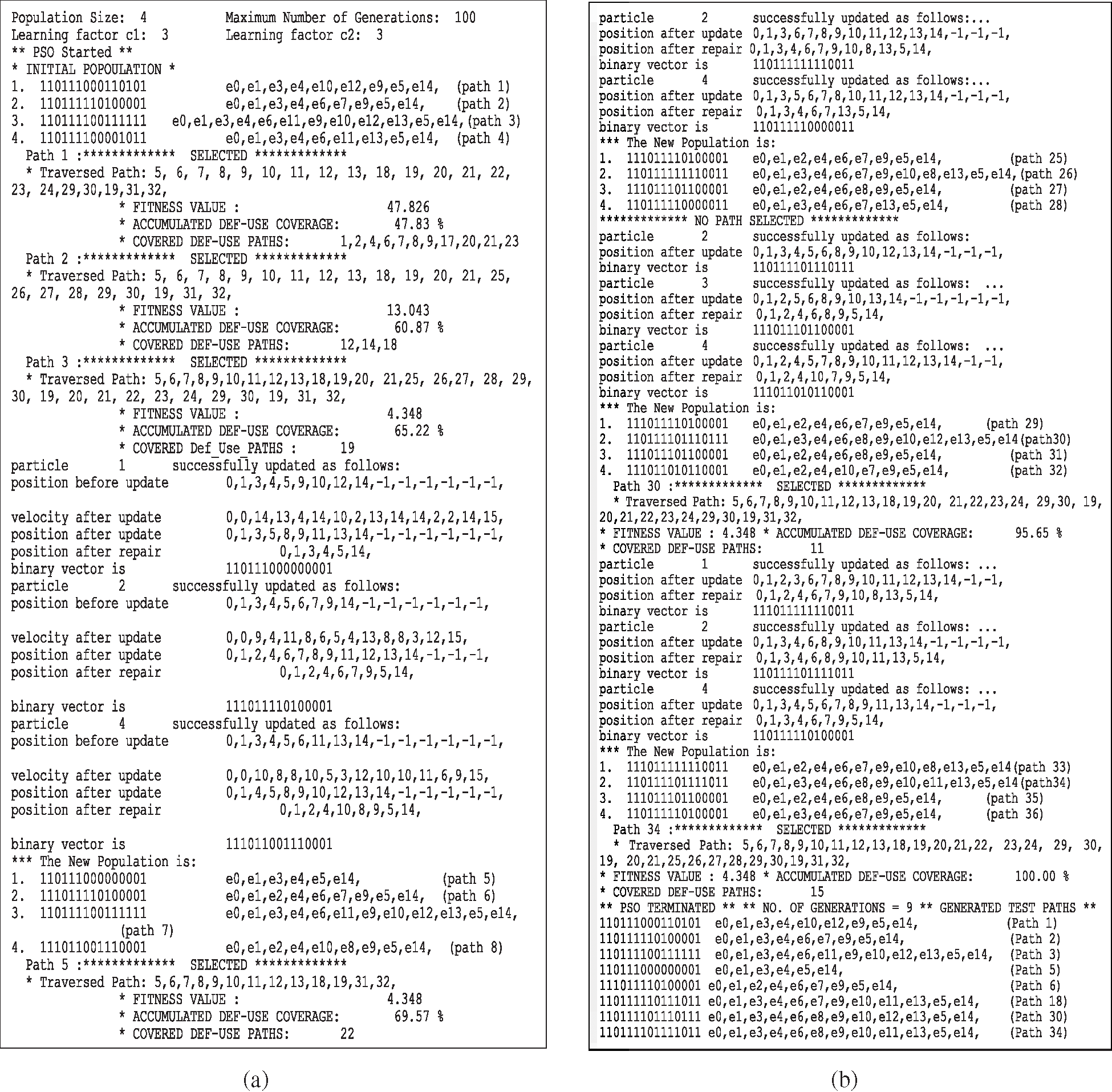
Figure 5: Part of the report of the path generation module
Fig. 7 compares the PSO-based system and the GA-based system according to the number of generations needed to cover all def-uses paths for every subject program. According to this comparison, the PSO system is more effective than the GA-based system in reducing the number of generations needed to accomplish 100% def-use path coverage.

Figure 6: The technique report for the 8 paths that covered all def-use pairs of the example program
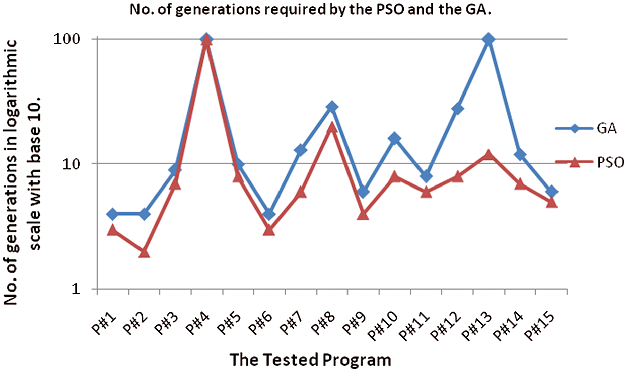
Figure 7: Number of generations of the GA-based and the PSO-based systems
Fig. 8 compares the PSO-based and the GA-based systems according to the number of paths created to satisfy all def-uses paths. The PSO-based technique generated 60 paths for satisfying 99.3% of all def-use paths, while the GA-based technique generated 63 paths to cover 98.6% of all def-use paths.

Figure 8: Number of paths created by the GA-based and the PSO-based systems
According to this comparison, the PSO-based system is more effective than the GA-based system in reducing the number of paths for 5 out of the 15 programs. In the other 9 programs, the two systems created an equal number of paths. In P#13 the GA-based system created a number of paths smaller than the PSO-based system but it reached only 91.11% coverage, while the PSO-based system reached 100% coverage.
This paper introduced a path-testing approach, which applies a PSO algorithm to construct test paths to satisfy the all-uses criterion. For programs that contain loops, the presented approach creates the paths according to the ZOT-criterion. An experiment that included 15 C# programs has been conducted to evaluate the efficiency of the presented technique compared to a GA-based path generation technique. The results showed that the PSO-based technique required 199 generations, while the GA-based technique needed 349 generations, to satisfy all def-uses of all programs. The PSO-based technique generated 60 paths and the GA-based technique generated 63 paths to satisfy all def-uses. In the future work, the experiments will be re-conducted to compare the time consumed by the two techniques using the same machine. Also, we will focus on conducting the experiments using another programing language such as Java with large data set. In addition, in the future work, we will focus on developing a system to find a set of test data to cover the generated paths.
Funding Statement: Taif University Researchers Supporting Project (TURSP) under number (TURSP-2020/73), Taif University, Taif, Saudi Arabia.
Conflicts of Interest: The authors declare that they have no conflicts of interest to report regarding the present study.
1. A. Bertolino andM. Marre, “Automatic generation of path covers based on the control flow analysis of computer programs,” IEEE Transactions on Software Engineering, vol. 20, no. 12, pp. 885–899, 1994. [Google Scholar]
2. T. McCabe, “Structural testing: A software testing methodology using the cyclomatic complexity metric.” NIST Special Publication 500-99, Washington D.C., 1982. [Google Scholar]
3. J. Poole, “A Method to Determine a Basis Set of Paths to Perform Program Testing, NIST Interagency/Internal Report (NISTIR)-5737, National Institute of Standards and Technology,” Gaithersburg, MD, 1995. Available:http://hissa.nist.gov//publications/nistir5737, last access 28-12-2020. [Google Scholar]
4. Z. Guangmei,C. Rui,L. Xiaowei andH. Congying, “The automatic generation of basis set of path for path testing,” inProceedings of 14th Asian Test Symposium (ATS’05Calcutta, India, pp. 46–51, 2005. [Google Scholar]
5. J. Yan andJ. Zhang, “An efficient method to generate feasible paths for basis path testing,” Information Processing Letters, vol. 107, no. 3–4, pp. 87–92, 2008. [Google Scholar]
6. Z. Zhonglin andM. Lingxia, “An improved method of acquiring basis path for software testing,” inProceedings of 5th International Conference on Computer Science & Education, Hefei, pp. 1891–1894, 2010. [Google Scholar]
7. D. Qingfeng andD. Xiao, “An improved algorithm for basis path testing,” inProceedings of 2011 International Conference on Business Management and Electronic Information, Guangzhou, pp. 175–178, 2011. [Google Scholar]
8. A. S. Ghiduk, “Automatic generation of basis test paths using variable length genetic algorithm,” Information Processing Letters, vol. 114, no. 6, pp. 304–316, 2014. [Google Scholar]
9. J. Kennedy andR. Eberhart, “Particle swarm optimization,” inProceedings of IEEE International Conference on Neural Networks, Perth, WA, Australia, pp. 1942–1948, 1995. [Google Scholar]
10. J. Kennedy, “Particle swarm optimization,” In: C. Sammut and G. I. Webb (eds.Encyclopedia of Machine Learning, Springer, Boston, MA, pp. 32–45, 2011. [Google Scholar]
11. K. Wang,L. Huang,C. Zhou andW. Pang, “Particle swarm optimization for traveling salesman problem,” inProceedings of the 2003 International Conference on Machine Learning and Cybernetics (IEEE Cat. No.03EX693Xi'an, vol. 3, pp. 1583–1585, 2003. [Google Scholar]
12. A. Li andY. Zhang, “Automatic generation method of test data for software structure based on PSO,” Computer Engineering, vol. 34, no. 6, pp. 93–97, 2008. [Google Scholar]
13. A. Li andY. Zhang, “Automatic generating all-path test data of a program based on PSO,” inThe 2009 WRI World Congress on Software Engineering (WCSE'09Los Alamitos: IEEE, pp. 189–193, 2009. [Google Scholar]
14. P. M. S. Bueno,W. E. Wong andM. Jino, “Automatic test data generation using particle systems,” inProceedings of the 2008 ACM Symposium on Applied Computing, pp. 809–814, 2008. [Google Scholar]
15. K. Agrawal andG. Srivastava, Towards software test data generation using discrete quantum particle swarm optimization. Mysore, India: ISEC, 65– 68, 2010. [Google Scholar]
16. N. Narmada andD. Mohapatra, “Automatic test data generation for data flow testing using particle swarm optimization,” Communications in Computer and Information Science, vol. 95, no. 1, pp. 1–12, 2010. [Google Scholar]
17. P. Nie,J. Geng andZ. Qin, “Multi-path oriented particle swarm optimization automatic test case generation algorithm,” Computer Integrated Manufacturing Systems, vol. 18, no. 1, pp. 216–223, 2012. [Google Scholar]
18. F. Almansour,R. Alroobaea andA. S. Ghiduk, “An empirical comparison of the efficiency and effectiveness of genetic algorithms and adaptive random techniques in data-flow testing,” IEEE Access, vol. 8, no. 1, pp. 12884–12896, 2020. [Google Scholar]
19. A. S. Ghiduk andS. Elzoughdy, “CHOMK: Concurrent higher-order mutants killing using genetic algorithm,” Arabian Journal for Science and Engineering, vol. 43, no. 12, pp. 7907–7922, 2018. [Google Scholar]
20. A. S. Ghiduk,M. R. Girgis andM. Hashim, “Reducing the cost of higher-order mutation testing,” Arabian Journal for Science and Engineering, vol. 43, no. 12, pp. 7473–7486, 2018. [Google Scholar]
21. A. S. Ghiduk, “Reducing the number of higher-order mutants with the aid of data flow,” e-Informatica Software Engineering Journal, vol. 10, no. 1, pp. 31–50, 2016. [Google Scholar]
22. M. R. Girgis,A. S. Ghiduk andE. H. Abd-Elkawy, “Automatic generation of data flow test paths using a genetic algorithm,” International Journal of Computer Applications, vol. 89, no. 12, pp. 29–36, 2014. [Google Scholar]
23. B. Hoseini andS. Jalili, “Automatic test path generation from sequence diagram using genetic algorithm,” inProceedings of 7'th International Symposium on Telecommunications (IST'2014Tehran, pp. 106–111, 2014. [Google Scholar]
24. K. Niveth andK. Vipin, “Automated test path generation using genetic algorithm,” International Journal of Engineering Research and Technology, vol. 6, no. 7, pp. 469–472, 2017. [Google Scholar]
25. A. Arwan andD. Sagita, “Determining basis test paths using genetic algorithm and J48,” International Journal of Electrical and Computer Engineering, vol. 8, no. 5, pp. 3333–3340, 2018. [Google Scholar]
26. A. Shanthi andG. Mohankumar, “Novel approach for automated test path generation using Tabu search algorithm,” International Journal of Computer Applications, vol. 48, no. 13, pp. 28–34, 2012. [Google Scholar]
27. P. Jain andA. Solanki, “A hybrid approach for test path generation and prioritization using depth first search and Tabu search algorithm,” Journal of Software Engineering Tools and Technology Trends, vol. 2, no. 2, pp. 7–20, 2015. [Google Scholar]
28. X. Bao,Z. Xiong,N. Zhang,J. Qian,B. Wuet al., “Path-oriented test cases generation based adaptive genetic algorithm,” PLoS One, vol. 12, no. 11, pp. e0187471, 2017. [Google Scholar]
29. A. A. Kyaw andM. M. Min, “Test path optimization algorithm compared with GA based approach,” inGenetic and Evolutionary Computing, Advances in Intelligent Systems and Computing, Cham: Springer, vol. 387, 2016. [Google Scholar]
30. M. Bures andB. S. Ahmed, “Employment of multiple algorithms for optimal path-based test selection strategy,” Information and Software Technology, vol. 114, no. 4, pp. 21–36, 2019. [Google Scholar]
31. V. N. S. Shailja Gupta, “Test path generation using cellular automata,” International Journal of Engineering and Computer Science, vol. 5, no. 6, pp. 16846–16854, 2016. [Google Scholar]
32. Haraty R. A.,Mansour N. andZeitunlian H., “Metaheuristic Algorithm for State-Based Software Testing,” Applied Artificial Intelligence, vol. 32, no. 2, pp. 197–213, 2018. [Google Scholar]
33. Haraty R. A.,Mansour N.,Moukahal L. andKhalil I., “Regression test cases prioritization using clustering and code change relevance,” International Journal of Software Engineering and Knowledge Engineering, vol. 26, no. 5, pp. 733–768, 2016. [Google Scholar]
34. H. A. Shaar andR. A. Haraty, “Modelling and automated blackbox regression testing of web applications,” Journal of Theoretical and Applied Information Technology, vol. 4, no. 12, pp. 1182–1198, ISSN: 1192-8645, 2008. [Google Scholar]
35. R. A. Haraty,N. Mansour andB. A. Daou, “Regression testing of database applications,” Journal of Database Management, vol. 13, no. 2, pp. 285–289, 2002. [Google Scholar]
36. S. Rapps andE. Weyuker, “Selecting software test data using data flow information,” IEEE Transactions on Software Engineering, vol. 11, no. 4, pp. 367–375, 1985. [Google Scholar]
37. M. R. Girgis, “An experimental evaluation of a symbolic execution system,” Software Engineering Journal, vol. 7, no. 4, pp. 285–290, 1992. [Google Scholar]
38. M. R. Girgis, “Using symbolic execution and data flow criteria to aid test data selection,” Journal of Software Testing, Verification and Reliability, vol. 3, no. 2, pp. 101–112, 1993. [Google Scholar]
39. S. Sengupta,S. Basak andR. Peters, “Particle swarm optimization: A survey of historical and recent developments with hybridization perspectives,” Machine Learning and Knowledge Extraction, vol. 1, no. 1, pp. 157–191, 2018. [Google Scholar]
40. R. Eberhart andY. Shi, “Comparing inertia weights and constriction factors in particle swarm optimization,” inProceedings of 2000 Congress on Evolutionary Computation, San Diego, CA, pp. 84–88, 2000. [Google Scholar]
41. M. Clerc, “The swarm and the queen: Towards a deterministic and adaptive particle swarm optimization,” inProceedings of 1999 Congress on Evolutionary Computation, Washington, DC, USA, pp. 1951–1957, 1999. [Google Scholar]
42. M. R. Girgis, “Automatic test data generation for data flow testing using a genetic algorithm,” Journal of Universal computer Science, vol. 11, no. 5, pp. 898–915, 2005. [Google Scholar]
43. A. S. Ghiduk andM. Rokaya, “An empirical evaluation of the subtlety of the data-flow based higher-order mutants,” Journal of Theoretical and Applied Information Technology, vol. 97, no. 15, pp. 4061–4074, 2019. [Google Scholar]
 | This work is licensed under aCreative Commons Attribution 4.0 International License, which permits unrestricted use, distribution, and reproduction in any medium, provided the original work is properly cited. |