Intelligent Automation & Soft Computing DOI:10.32604/iasc.2021.018111
Article

Inference on Generalized Inverse-Pareto Distribution under Complete and Censored Samples

Abdelaziz Alsubie1, Mostafa Abdelhamid2, Abdul Hadi N. Ahmed2, Mohammed Alqawba3 and Ahmed Z. Afify4,*

1Department of Basic Sciences, College of Science and Theoretical Studies, Saudi Electronic University, Riyadh, 11673, Saudi Arabia
2Department of Mathematical Statistics, Faculty of Graduate Studies for Statistical Research, Cairo University, Giza, 12631, Egypt
3Department of Mathematics, College of Science and Arts, Qassim University, Ar Rass, 51921, Saudi Arabia
4Department of Statistics, Mathematics and Insurance, Benha University, Benha, 13511, Egypt
*Correspondence: Ahmed Z. Afify. Email: ahmed.afify@fcom.bu.edu.eg
Received: 21 February 2021; Accepted: 25 March 2021

Abstract: In this paper, the estimation of the parameters of extended Marshall-Olkin inverse-Pareto (EMOIP) distribution is studied under complete and censored samples. Five classical methods of estimation are adopted to estimate the parameters of the EMOIP distribution from complete samples. These classical estimators include the percentiles estimators, maximum likelihood estimators, least squares estimators, maximum product spacing estimators, and weighted least-squares estimators. The likelihood estimators of the parameters under type-I and type-II censoring schemes are discussed. Simulation results were conducted, for various parameter combinations and different sample sizes, to compare the performance of the EMOIP estimation methods under complete and censored samples. Further, the mean square errors, asymptotic confidence interval, average interval length, and coverage percentage are calculated under the two censored schemes. The simulation results illustrate that the coverage probabilities of the confidence intervals increase to the nominal levels when the sample size increases. A real data set from the insurance field is analyzed for illustrative purposes. The data represent monthly metrics on unemployment insurance from July 2008 to April 2013 and contain 21 variables and particularly we study the variable number 11 in the data. The EMOIP model provides a better fit as compared with the inverse-Pareto distribution under complete and censored schemes. We hope that the EMOIP distribution will attract wider applications in the insurance field which contains several heavy-tailed real data.

Keywords: Inverse-Pareto distribution; censored samples; insurance data; percentile estimators; Marshall-Olkin family; simulation

1  Introduction

In statistical literature, many standard distributions are used when studying real data in different applied fields, but the known standard distributions are limited comparing with various real data. There is increased interest of finding new distributions by extending the existing ability of studying the unlimited range of the real data. Marshall et al. [1] introduced an important method of adding an extra parameter to well-known existing distributions, which gives more flexibility to model various types of data. The resulting distribution includes the baseline distribution as a special case when the new added parameter equals one. Their method is called the Marshall-Olkin (MO) family.

In this paper, the estimation of the extended Marshall-Olkin inverse-Pareto (EMOIP) parameters is conducted using five classical estimators, including the maximum likelihood estimators (MLEs), least squares estimators (LSEs), weighted least-squares estimators (WLSEs), percentiles estimators (PCEs), and maximum product spacing estimators (MPSEs). The behavior of these estimators is addressed using extensive simulation results for small and large samples. Furthermore, we address the estimation of the EMOIP parameters under censoring schemes, including type I censoring and type II censoring schemes. We have also conducted a Monte Carlo simulation study to calculate the MLEs for the unknown parameters under type I and type II censoring schemes. Finally, we analyze real data from the insurance field for illustrative purposes.

The EMOIP model was introduced by Gharib et al. [2] to model data with unimodal hazard rate function (HRF). They derived some basic distributional properties, including the quantile function, ordinary moments, incomplete moments, negative moments, moments of residual life and reversed residual life, and order statistics.

Gharib et al. [2] extended the Inverse-Pareto (IP) distribution, as a baseline distribution, to obtain their new distribution, which is called the Extended Marshall-Olkin Inverse-Pareto (EMOIP). The EMOIP model is obtained by applying the MO transformation, which is defined by the following survival function (SF)

F¯(x;δ)=δG¯(x)1−δ¯G¯(x),−∞<x<∞,δ>0,δ¯=1−δ. (1)

Or the cumulative distribution function (CDF)

F(x;δ)=1−δ[1−G(x)]δ−(δ−1)G(x).

If G¯(x) is the IP SF, for δ=1 , we obtain the baseline model, i.e., F¯(x)=G¯(x) or F(x)=G(x) .

The MO family is one of the most common generators in the literature and has been used extensively to extend several classical distributions as well as several other families of distributions. The most notable recent works include the MO extended-Weibull [3], MO generalized Burr-XII [4], MO exponentiated Burr-XII [5], MO additive-Weibull [6], Marshall-Olkin power Lomax [7], and MO power generalized-Weibull [8] distributions, among many others, including the MO alpha-power family [9], MO Burr-R class [10], and MO Burr-III family [11].

The two-parameter IP distribution [12, P. 707, Sec. A.2.3.2] is specified by the following CDF

G(x;α,β)=(xx+β)α,x>0, (2)

in which α and β are positive shape parameters.

The probability density function (PDF) of the IP distribution has the form

g(x;α,β)=αβxα−1(β+x)α+1,x>0. (3)

The CDF of the EMOIP distribution with three parameters, α,β and δ for (x>0) , is given as

F(x;α,β,δ)={1−δ[1−(xx+β)α]δ−(δ−1)(xx+β)αifx>0;α,β,δ>0,δ≠1,(xx+β)αifx>0;α,β,δ>0,δ=1. (4)

in which α,β and δ are shape parameters.

The PDF of the EMOIP distribution reduces to

f(x;α,β,δ)={αβδxα−1(x+β)−α−1[δ−(δ−1)(xx+β)α]2ifx>0;α,β,δ>0,δ≠1,αβδxα−1(x+β)−α−1ifx>0;α,β,δ>0,δ≠1. (5)

Clearly, for δ=1 , we obtain the IP(α,β) distribution. Fig. 1 displays some shapes for the density and hazard functions of the EMOIP distribution.

The HRF of the EMOIP model is given as

h(x;α,β,δ)=αβ(xx+β)αx(x+β)[1−(xx+β)α][δ−(δ−1)(xx+β)α].

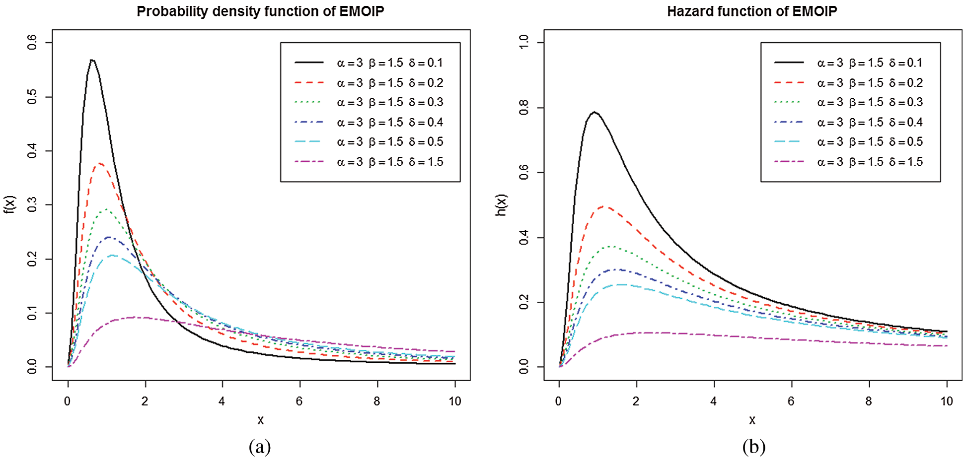
Figure 1: (a) Some plots of the PDF of the EMOIP model; (b) Some plots of the HRF of the EMOIP model

The rest of the article is organized in four sections. Section 2 describes five classical estimation methods for estimating the EMOIP parameters and examines the proposed estimators numerically via Monte Carlo simulations. Section 3 discusses the estimation under censored samples as well as provides a detailed simulation study. A real data set from the insurance science is analyzed in Section 4 for illustrative purposes. Finally, Section 5 is devoted to the conclusion.

2  Estimation Under Complete Samples with Simulations

This section is devoted to estimating the parameters α , β and δ of the EMOIP distribution using five estimators: MLEs, LSEs, WLSEs, PCEs, and MPSEs. These estimation methods were adopted in the literature to estimate the unknown parameters of several distributions. For example, the alpha logarithmic transformed Weibull [13], quasi xgamma-geometric [14], logarithmic transformed Weibull [15], Weibull Marshall–Olkin Lindley [16], generalized Ramos–Louzada [17], Fréchet [18], heavy-tailed exponential [19], and inverse weighted Lindley [20] distributions.

2.1 Maximum Likelihood Estimation

Let x1,…,xn be a random sample from the EMOIP model and let x(1)<x(2)<…<x(n) be the associated order statistics. The log-likelihood function reduces to

L(α,β,δ)=nln⁡(α)+nln⁡(β)+nln⁡(δ)+(α−1)∑i=1nln(xi)−(α+1)∑i=1nln(xi+β)−2∑i=1nln[δ−(δ−1)(xixi+β)α]. (6)

The MLEs of the EMOIP parameters α , β and δ can be obtained by differentiating Eq. (6) and equating the results to zero. The resulting equations are

∂L(α,β,δ)∂α=nα+∑i=1nln(xi)−∑i=1nln(xi+β)+2∑i=1n1ψi[(δ−1)(xixi+β)αln⁡(xixi+β)]=0

and

∂L(α,β,δ)∂δ=nδ−2∑i=1n1ψi[1−(xixi+β)α]=0,

in which ψi=δ−(δ−1)(xixi+β)α.

The MLEs of α , β and δ , say α^ , β^ and δ^ can be obtained by solving the last three non-linear equations simultaneously.

2.2 Percentile Estimation

The percentiles estimation method is introduced by Kao et al. [21,22]. The PCEs of the parameters α , β and δ of the EMOIP model can be determined by minimizing the following function:

∑i=1n{x(i)−β[(1+(δ−1)p(i)δp(i))1α−1]−1}2, (7)

with respect to α , β and δ . Further, the PCEs of α , β and δ can be obtained by solving the following equations:

∑i=1n{x(i)−β[(1+(δ−1)p(i)δp(i))1α−1]−1}ρl(x(i)|α,β,δ)=0,l=1,2,3,

where

ρ1(x(i)|α,β,δ)=[(1+(δ−1)p(i)δp(i))1α−1]−2(1+(δ−1)p(i)δp(i))1αln(1+(δ−1)p(i)δp(i)),

ρ2(x(i)|α,β,δ)=[(1+(δ−1)p(i)δp(i))1α−1]−1

and

ρ3(x(i)|α,β,δ)=[(1+(δ−1)p(i)δp(i))1α−1]−2(1+(δ−1)p(i)δp(i))1−ααp(i)−1p(i).

2.3 Least Squares and Weighted Least Squares Estimation

The LSEs and WLSEs are adopted to estimate the beta parameters [23]. The LSEs of the parameters α , β and δ of the EMOIP distribution are obtained by minimizing the following function with respect to α , β and δ .

∑i=1n[(1−δ(1−(x(i)x(i)+β)α)δ−(δ−1)(x(i)x(i)+β)α)−in+1]2. (8)

These estimates can also be obtained by solving the following nonlinear equations:

∑i=1n[(1−δ(1−(x(i)x(i)+β)α)δ−(δ−1)(x(i)x(i)+β)α)−in+1]λk(x(i)|α,β,δ)=0,k=1,2,3,

where

λ1(x(i)|α,β,δ)=ψ(i)δ(x(i)x(i)+β)αln(x(i)x(i)+β)+δ[1−(x(i)x(i)+β)α](1−δ)(x(i)x(i)+β)αln(x(i)x(i)+β)(ψ(i))2, (9)

λ2(x(i)|α,β,δ)=−ψ(i)δx(i)αα(x(i)+β)−α−1−δ[1−(x(i)x(i)+β)α](δ−1)x(i)αα(x(i)+β)−α−1(ψ(i))2 (10)

and

λ3(x(i)|α,β,δ)=ψ(i)[(x(i)x(i)+β)α−1]−δ[1−(x(i)x(i)+β)α].[1−(x(i)x(i)+β)α](ψ(i))2. (11)

The WLSEs of the EMOIP parameters α , β and δ can be calculated by minimizing the following function with respect to α , β and δ .

∑i=1n(n+1)2(n+2)n−i+1[(1−δ(1−(x(i)x(i)+β)α)δ−(δ−1)(x(i)x(i)+β)α)−in+1]2. (12)

Further, the WLSEs are obtained by solving the following equations:

∑i=1n(n+1)2(n+2)n−i+1[(1−δ(1−(x(i)x(i)+β)α)δ−(δ−1)(x(i)x(i)+β)α)−in+1]λk∖left(x(i)|α,β,δ)=0,k=1,2,3,

in which λ1(x(i)|α,β,δ) , λ2(x(i)|α,β,δ) and λ3(x(i)|α,β,δ) are defined in Eqs. (9)–(11).

2.4 Maximum Product of Spacings Estimation

The maximum product of spacings (MPS) method is proposed by Cheng et al. [24,25] to estimate the model parameters instead of the maximum likelihood.

The MPSEs of the EMOIP parameters α , β and δ can be calculated by maximizing the following function with respect to α , β and δ .

1n+1∑i=1n+1lnDi(α,β,δ),

where Di(α,β,δ)=F(x(i)|α,β,δ)−F(x(i−1)|α,β,δ),i=1,2,…,n .

Alternatively, these estimates can be obtained by solving the following equations:

1n+1∑i=1n+11Di(α,β,δ)[λk(x(i)|α,β,δ)−λk(x(i−1)|α,β,δ)]=0,k=1,2,3,

in which λ1(x(i)|α,β,δ) , λ2(x(i)|α,β,δ) and λ3(x(i)|α,β,δ) are defined in Eqs. (9)–(11).

2.5 Simulation Study

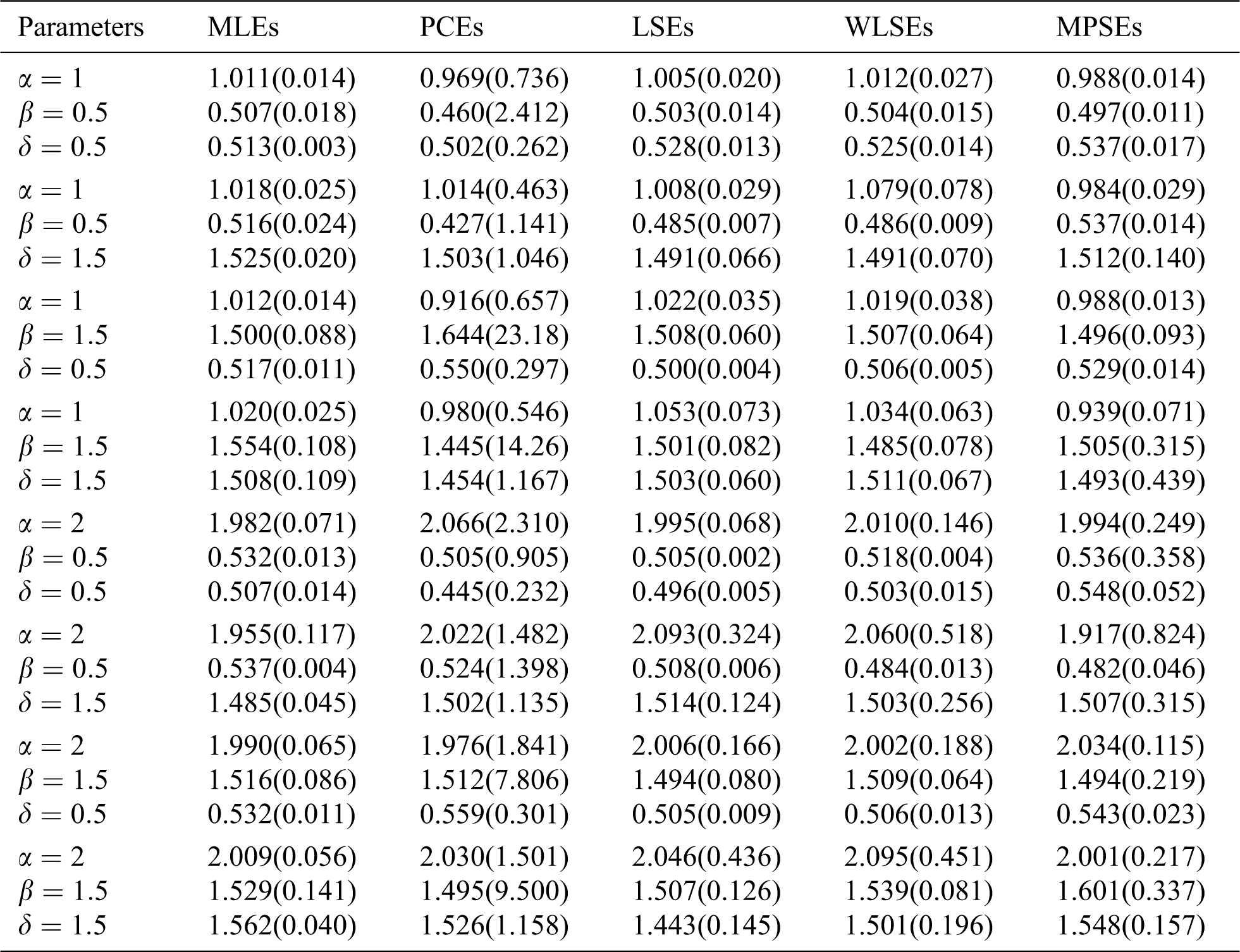
In this section, a Monte Carlo simulation study is conducted to compare the performance of the different estimators of the unknown parameters of the EMOIP distribution. The numerical results are obtained using the Mathcad program, version 14.0, to compare the performances of different estimators with respect to their mean squared errors (MSEs). We generate 2000 samples of the EMOIP distribution for n=(20,50,100,200) , α=(1,2) , β=(0.5,1.5) and δ=(0.5,1.5) .

The average values of estimates (AVEs) and MSEs of MLEs, LSEs, WLSEs, PCEs, and MPSEs are displayed in Tabs. 1–4. From Tabs. 1–4, the MSEs decrease as sample size increases. Comparing the different methods of estimation, the results show that the MLE produces the best results for estimating the parameters α , β and δ , in terms of MSEs in most of the studied cases. The ordering performance of the estimators in terms of MSEs (from best to worst) for α is MLE, MPSE, LSE, WLSE, and PCE. The ordering performance for β is MLE, WLSE, LSE, MPSE, and PCE, whereas the ordering performance is MLE, LSE, WLSE, MPSE, and MLE for the parameter δ .

3  Estimation Under Censored Samples

In this section, we address the MLEs of the EMOIP parameters under type-I and type-II censored samples. We derive the approximate confidence intervals of the unknown parameters from the Fisher information matrix under type-I and type-II censored samples. Finally, we perform a simulation study to explore the behavior of the estimates. Several authors have been studied the estimation of the model parameters under different censoring schemas, such as Tomazella et al. [26] and Alshenawy et al. [27].

3.1 Maximum Likelihood under Type-I Censored Sample

In censoring of type-I, the unit i is followed for a fixed time xoi , i=1,2,…,n , and the number of failures in the sample is random, say s units, where s=∑i=1ndi , and di is the death indicator, taking the value 1 if unit i dies and the value is 0 otherwise. Hence, the likelihood function L takes the form

L=∏i=1nf(xi)diS(xi)1−di,

Table 1: The AVEs and their corresponding MSEs (in parentheses) for n=20 .

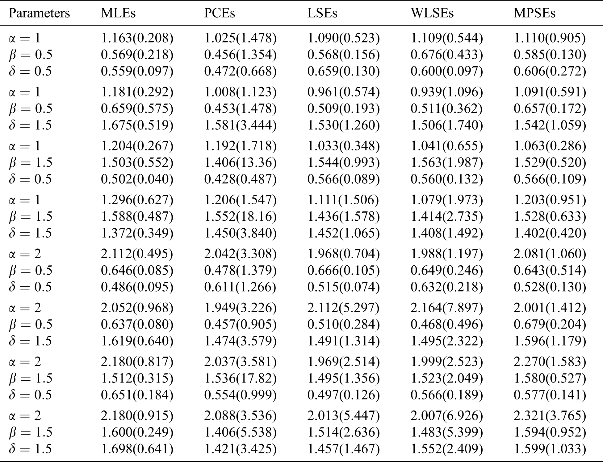
Table 2: The AVEs and their corresponding MSEs (in parentheses) for n=50 .

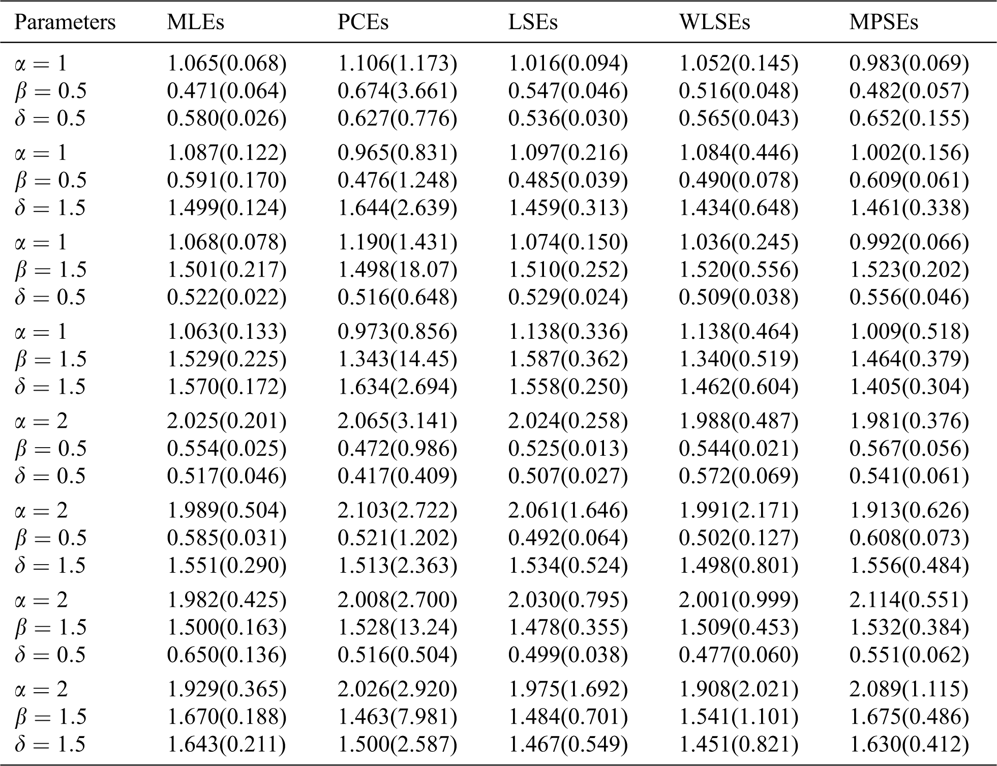
Table 3: The AVEs and their corresponding MSEs (in parentheses) for n=100 .

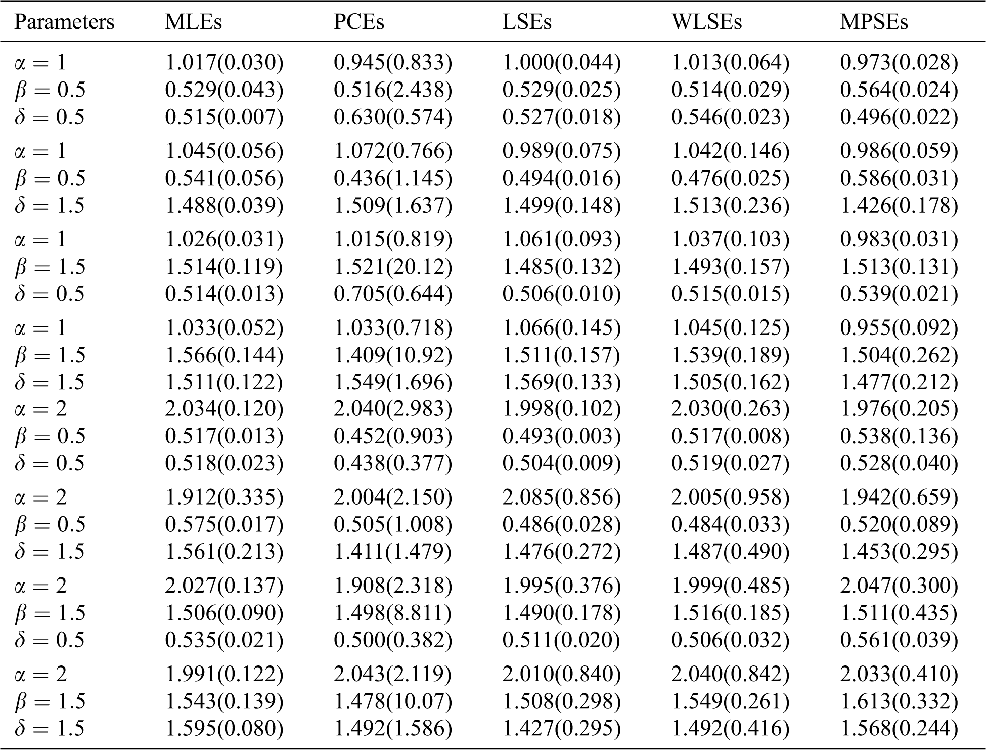
Table 4: The AVEs and their corresponding MSEs (in parentheses) for n=200 .

in which

di={1ifxi=xoi,0otherwise.

Therefore,

ln⁡L=∑i=1ndiln⁡f(xi)+∑i=1n(1−di)ln⁡S(xi).

Suppose that the fixed observation times for all units are equal to xo , then

ln⁡L=∑i=1ndiln⁡f(xi)+(n−s)ln⁡S(xo),s=∑i=1ndi,xi≤xo.

If X∼EMOIP(α,β,δ) , then ln⁡L for sample j(j=1,2,..,N) , N=1000 is:

ln⁡L=∑i=1ndiln⁡{αβδxi,jα−1(xi,j+β)−(α+1)[δ−(δ−1)(xi,jxi,j+β)α]2}+(n−sj)ln⁡{δ[1−(xojxoj+β)α]δ−(δ−1)(xojxoj+β)α}. (13)

The MLEs of α,β and δ under type-I censored sample are the solutions of the following three equations.

∂ln⁡L∂α=∑i=1ndi,j[1α+ln⁡xi,j−ln⁡(xi,j+β)+2(δ−1)(xi,jxi,j+β)αln⁡(xi,jxi,j+β)δ−(δ−1)(xi,jxi,j+β)α]−(n−sj)[(xojxoj+β)αln⁡(xojxoj+β)1−(xojxoj+β)α+(δ−1)(xojxoj+β)αln⁡(xojxoj+β)δ−(δ−1)(xojxoj+β)α],

∂lnL∂β=∑i=1ndi,j[1β−α+1xi,j+β−2α(δ−1)(xi,jxi,j+β)αδ−(δ−1)(xi,jxi,j+β)α(xi,j+β)]+(n−sj){α(xojxoj+β)α[1−(xojxoj+β)α](xoj+β)−α(δ−1)(xojxoj+β)α[δ−(δ−1)(xojxoj+β)α](xoj+β)}

and

∂lnL∂δ=∑i=1ndi,j{1δ−2[1−(xi,jxi,j+β)α]δ−(δ−1)(xi,jxi,j+β)α}+(n−sj)[1δ−1−(xojxoj+β)αδ−(δ−1)(xojxoj+β)α].

By solving the following equations simultaneously ∂ln⁡L∂α=0,∂ln⁡L∂β=0,∂ln⁡L∂δ=0, we obtain the MLEs α^ , β^ and δ^ .

3.2 Maximum Likelihood under Type-II Censored Sample

Let x1,…,xn be a random sample of size n from the EMOIP model and x1:r:n,…,xr:r:n be the censored data. It is known that we observe only the first r order statistics in the type-II censoring scheme; hence, the likelihood function, L, takes the form

L=C∏i=1rf(xi:r:n)[1−F(xr:r:n)]n−r.

For simplicity of notation, we use xi=xi:r:n,i=1,2,…,r and xr is the time of the r th failure. Then, log-likelihood function, without the constant term, follows as

ln⁡L=rlog⁡(αβδ)+∑i=1rln{xiα−1(xi+β)−(α+1)[δ−(δ−1)(xixi+β)α]2}+(n−r)ln⁡{δ[1−(xrxr+β)α]δ−(δ−1)(xrxr+β)α}. (14)

The MLEs of α,β and δ are the solution of the following three equations, which are the partial derivatives of Eq. (14) with respect to α,β and δ .

∂ln⁡L∂α=rα+(α−1)∑i=1rlnxi−(α+1)∑i=1rln(xi+β)−2∑i=1r(δ−1)(xixi+β)αln⁡(xixi+β)δ−(δ−1)(xixi+β)α−(n−r)[(xrxr+β)αln⁡(xrxr+β)1−(xrxr+β)α+(δ−1)(xrxr+β)αln⁡(xrxr+β)δ−(δ−1)(xrxr+β)α],

∂ln⁡L∂β=rβ+−(xi+β)−(α+1)∑i=1r(xi+β)−(α+2)−2∑i=1rα(δ−1)(xixi+β)αδ−(δ−1)(xixi+β)α(xi+β)+(n−r){α(xrxr+β)α[1−(xrxr+β)α](xr+β)−α(δ−1)(xrxr+β)α[δ−(δ−1)(xrxr+β)α](xr+β)}

and

∂ln⁡L∂δ=rδ−2∑i=1r1−(xixi+β)αδ−(δ−1)(xixi+β)α+(n−r)[1δ−1−(xrxr+β)αδ−(δ−1)(xrxr+β)α].

The above three equations cannot be solved explicitly, so the numerical techniques can be employed to obtain the MLEs of the parameters, i.e., α^ , β^ and δ^ .

3.3 Simulation Results

In this section, we conduct a simulation study to explore the performance of the MLEs of the EMOIP parameters in terms of their MSEs, asymptotic confidence interval (ACI), average interval length (AIL), and coverage percentage (CP) under type-I and type-II censored samples. We consider the values 20, 50, 100 and 200 for n and q=30%,60%,90%,100% (for type-I censoring) and r=30%,60%,90%,100% (for type-II censoring). For illustrative purposes and to keep the paper at adequate length, we chose only one combination of the parameters, α=2,β=0.05,δ=2 .

All simulation results are carried out using the R software, where we generate n=20,50,100,200 values from the EMOIP distribution with parameters α,β and δ using its quntile function and replicate the process N = 10,000 times to calculate the AVEs, MSEs, ACI, AIL, and CP.

The simulation results, including the AVEs, MSEs, ACI, AIL, and CP, are displayed in Tabs. 5–12. From Tabs. 5–12, we observe that the MSEs decrease as the sample size increases in all the cases under type-I and type-II censored samples. Furthermore, the AVEs tend to the true parameter values as n increases. In addition, in the case of type-I and type-II censored samples, the MSEs decrease in all the cases, and the estimates tend to the true parameter values as the number of failures q and r increase, respectively.

Table 5: The AVEs, MSEs, ACI, AILs and CPs of the EMOIP distribution under type-I censoring with q=30%

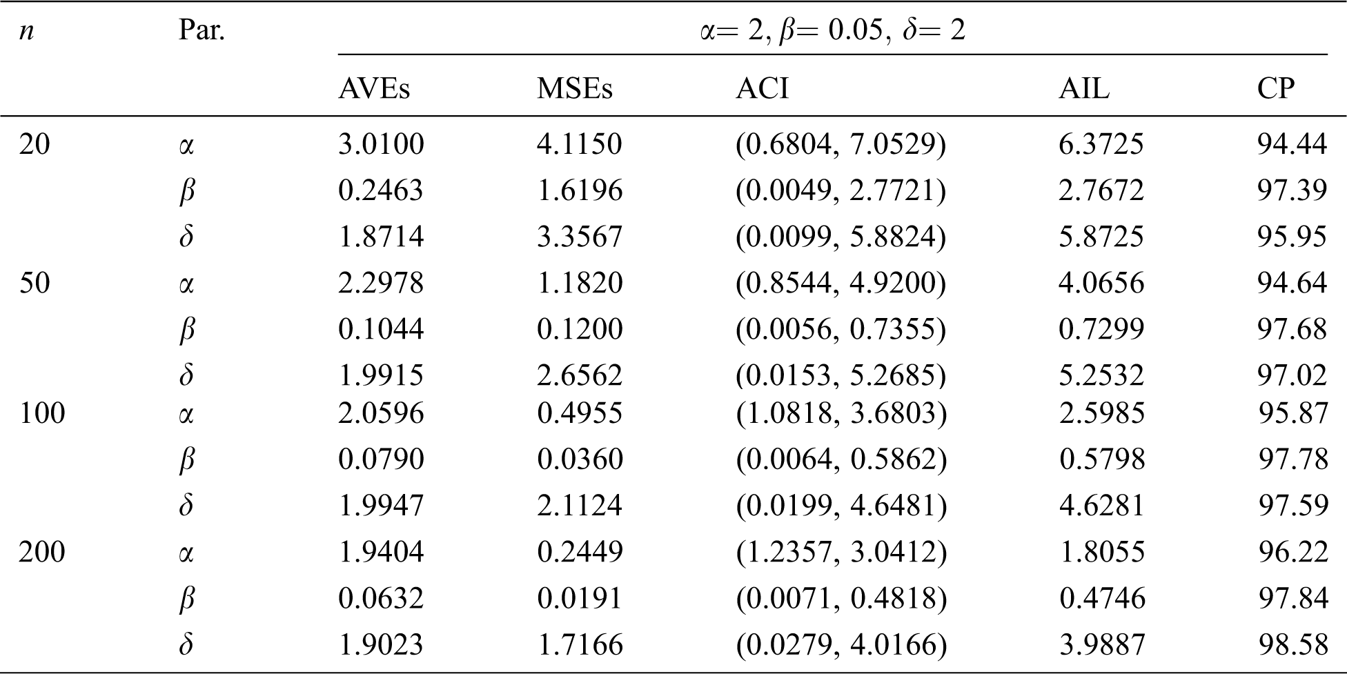
Table 6: MLE estimated, interval estimates, MSEs, AILs and CPs (in %) of EMOIP distribution under type-I censoring with q=60%

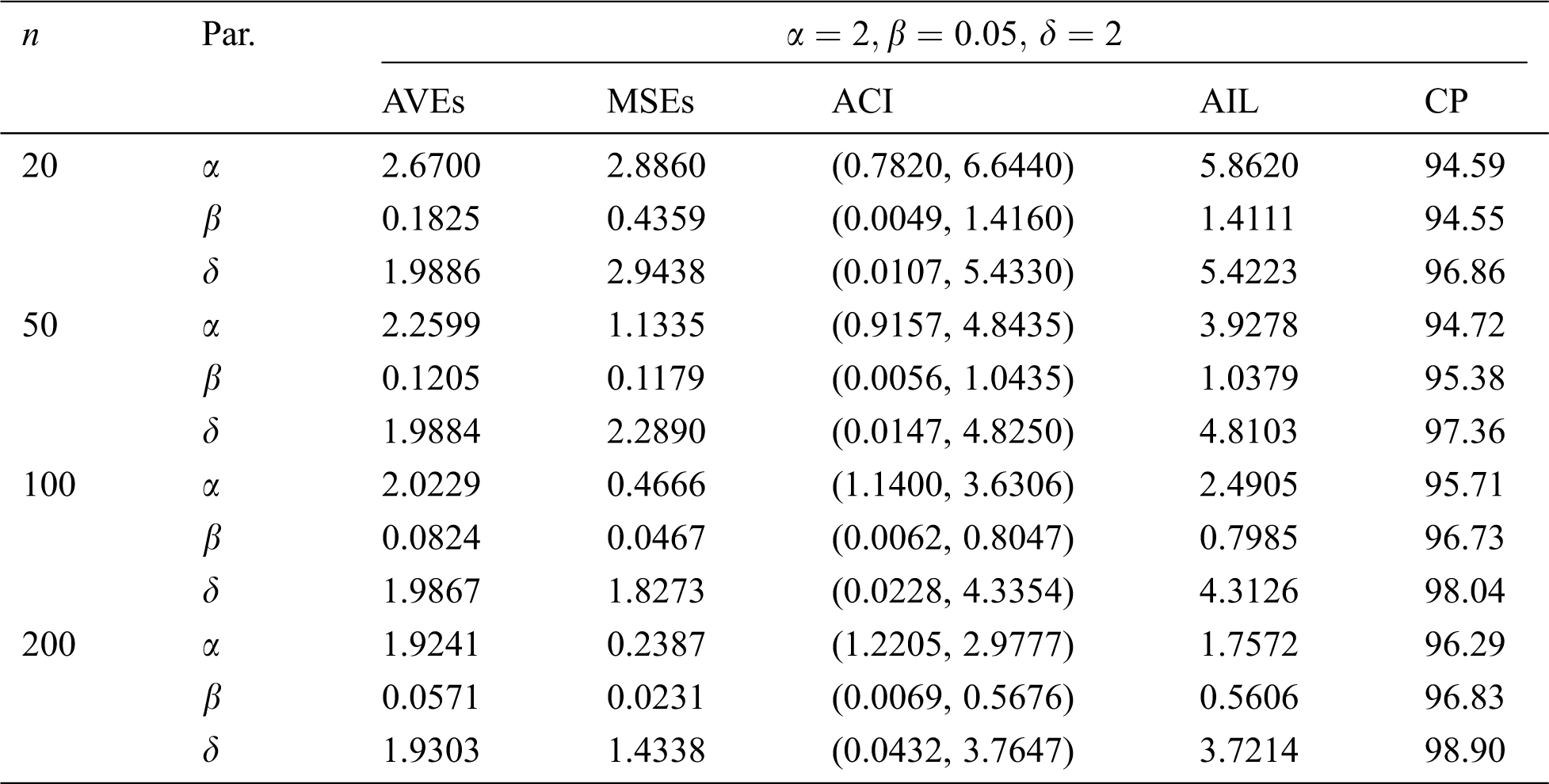
Table 7: MLE estimated, interval estimates, MSEs, AILs and CPs (in %) of EMOIP distribution under type-I censoring with q=90%

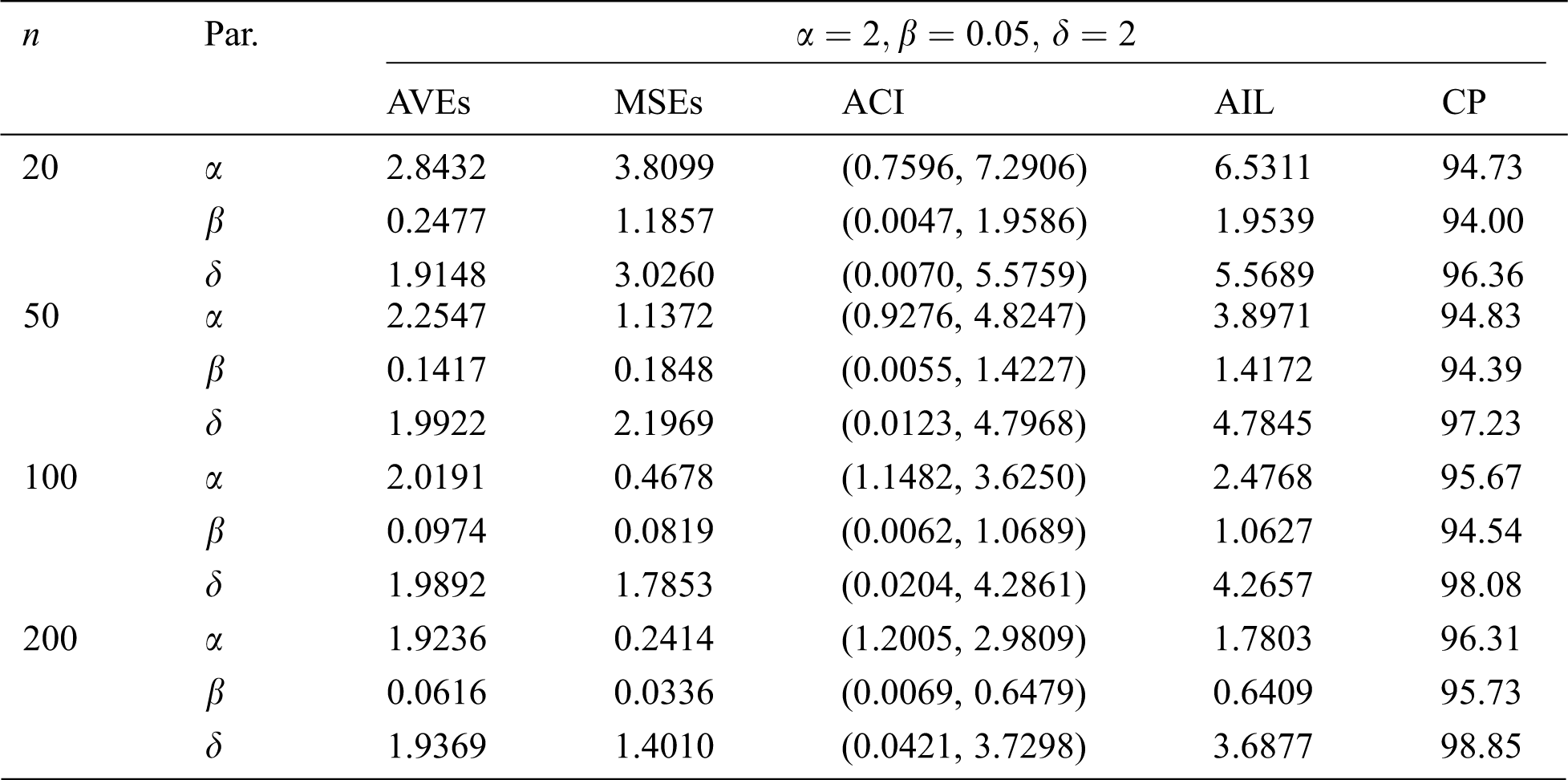
Table 8: MLE estimated, interval estimates, MSEs, AILs and CPs (in %) of EMOIP distribution under type-I censoring with q=100%

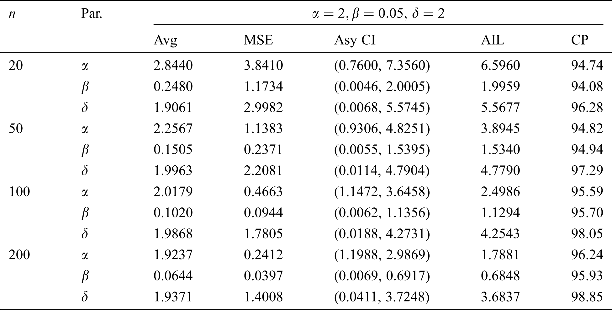
Table 9: MLE estimated, interval estimates, MSEs, AILs and CPs (in %) of EMOIP distribution under type-II censoring with r=30%

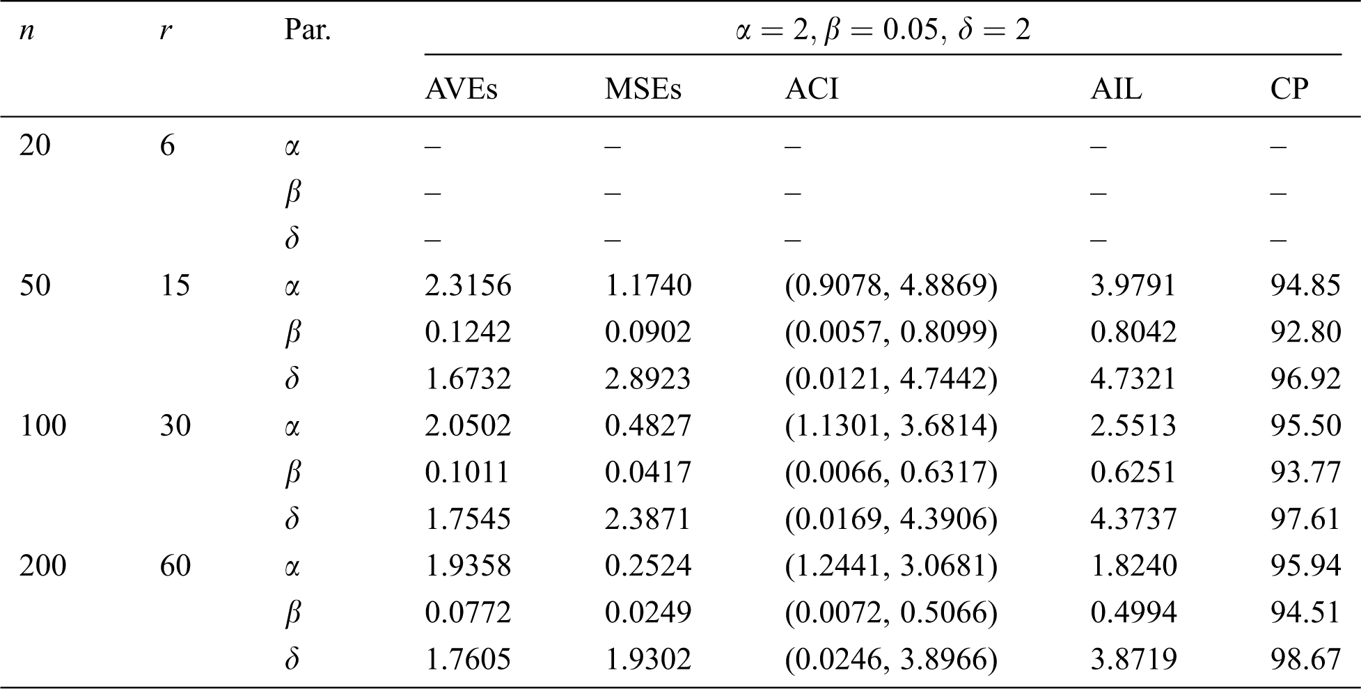
Table 10: MLE estimated, interval estimates, MSEs, AILs and CPs (in %) of EMOIP distribution under type-II censoring with r=60%

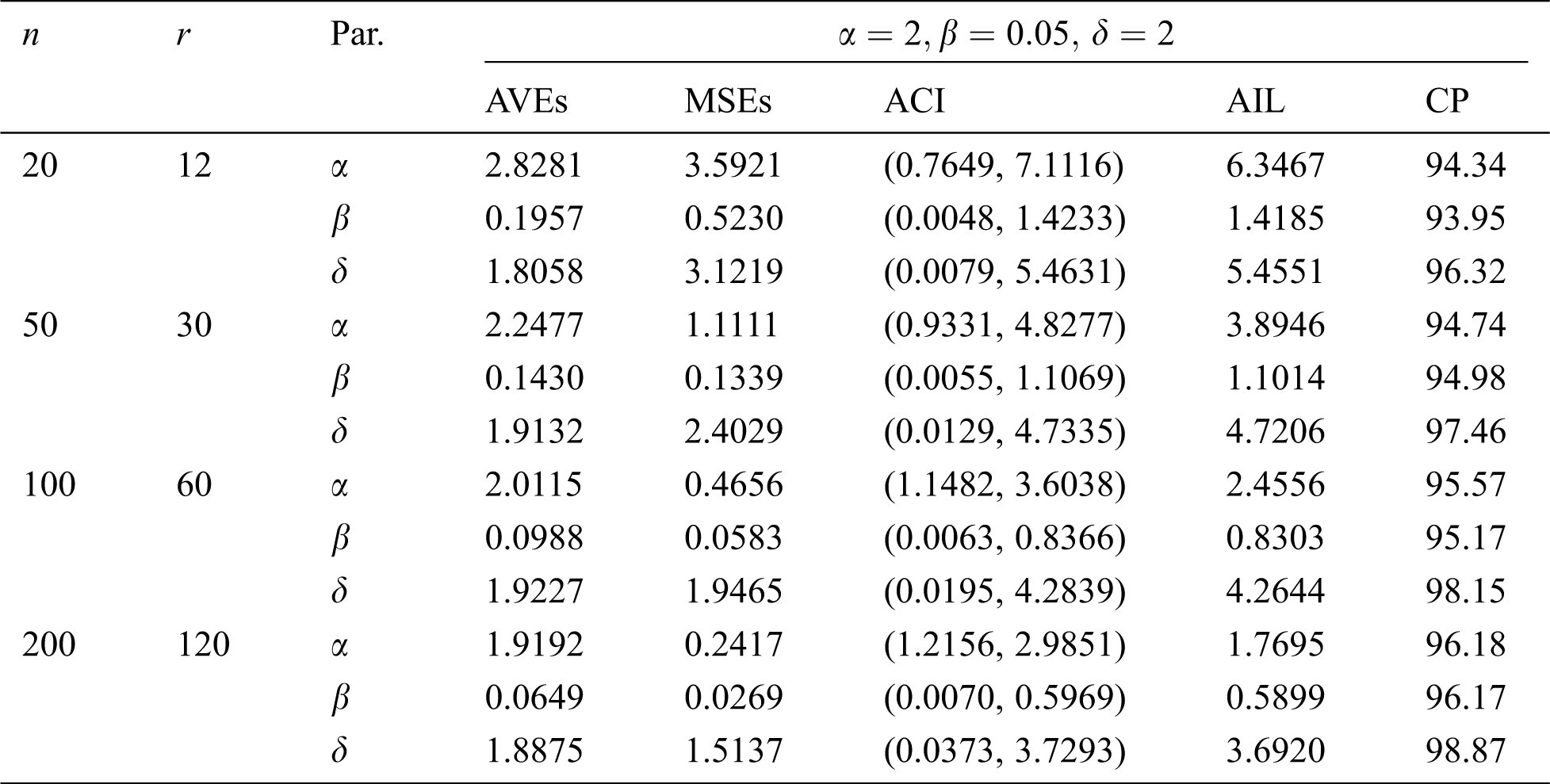
Table 11: MLE estimated, interval estimates, MSEs, AILs and CPs (in %) of EMOIP distribution under type-II censoring with r=90%

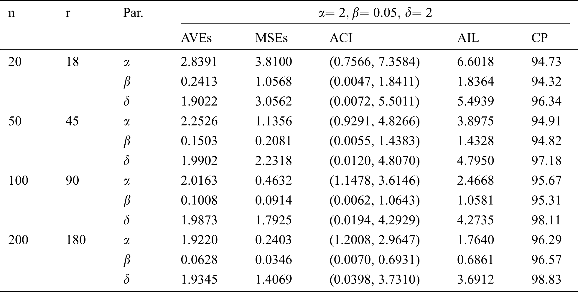
Table 12: MLE estimated, interval estimates, MSEs, AILs and CPs (in %) of EMOIP distribution under type-II censoring with r=100%

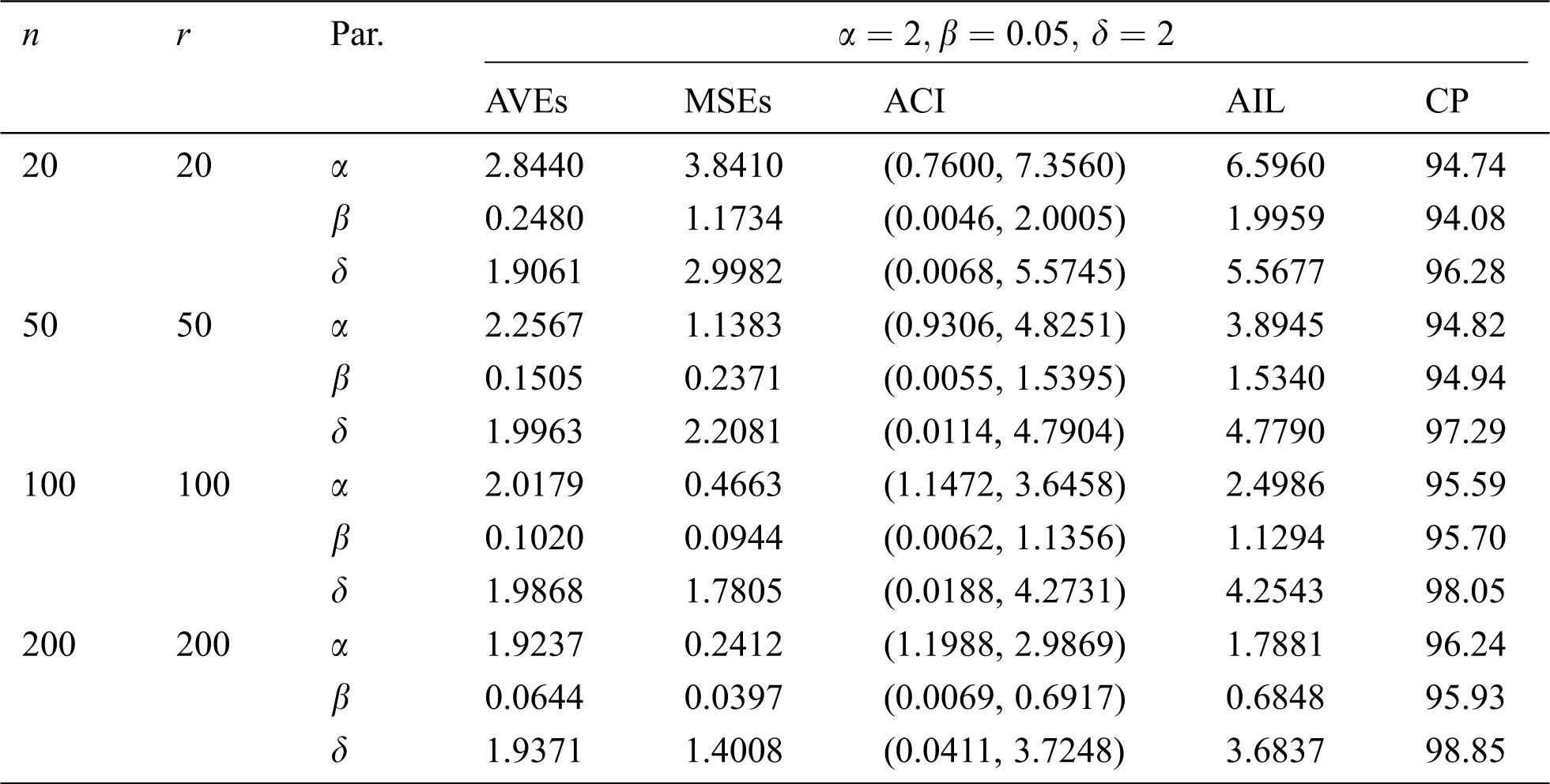
The results show that the MLEs of the EMOIP parameters under type-I and type-II schemes are asymptotically unbiased and consistent. As expected, the performance of the estimates under complete samples is better than those under type-I and type-II censored samples in terms of the MSEs. Furthermore, the AIL decreases as n increases under the complete and censored schemes in all the studied cases. The AIL in the case of complete samples are smaller than censored samples under type-I and type-II.

4  Real Data Analysis

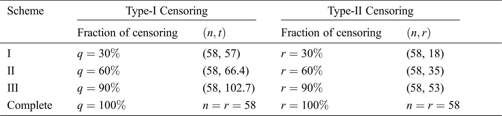
In this section, we analyze a real data set for illustrative purpose. The following data set represents monthly metrics on unemployment insurance from July 2008 to April 2013 as reported by the department of Labor, Licensing and Regulation, State of Maryland, USA. The data set contains 21-variable and here we consider the variable number 11 in the data file which is available at: https://catalog.data.gov/dataset/unemployment-insurance-data-july-2008-to-april-2013. The data contain 58 observations: 29, 32, 33, 36, 39, 41, 44, 50, 50, 50, 52, 52, 52, 52, 53, 54, 56, 57, 57, 57, 58, 59, 60, 60, 60, 61, 61, 61, 63, 64, 64, 64, 65, 66, 66, 68, 68, 69, 69, 70, 72, 73, 74, 75, 80, 80, 80, 83, 90, 90, 95, 100, 109, 114, 133, 137, 170, 222. The EMOIP parameters are estimated using the maximum likelihood (ML) method under the following schemes for type-I and type-II censoring as follows:

:

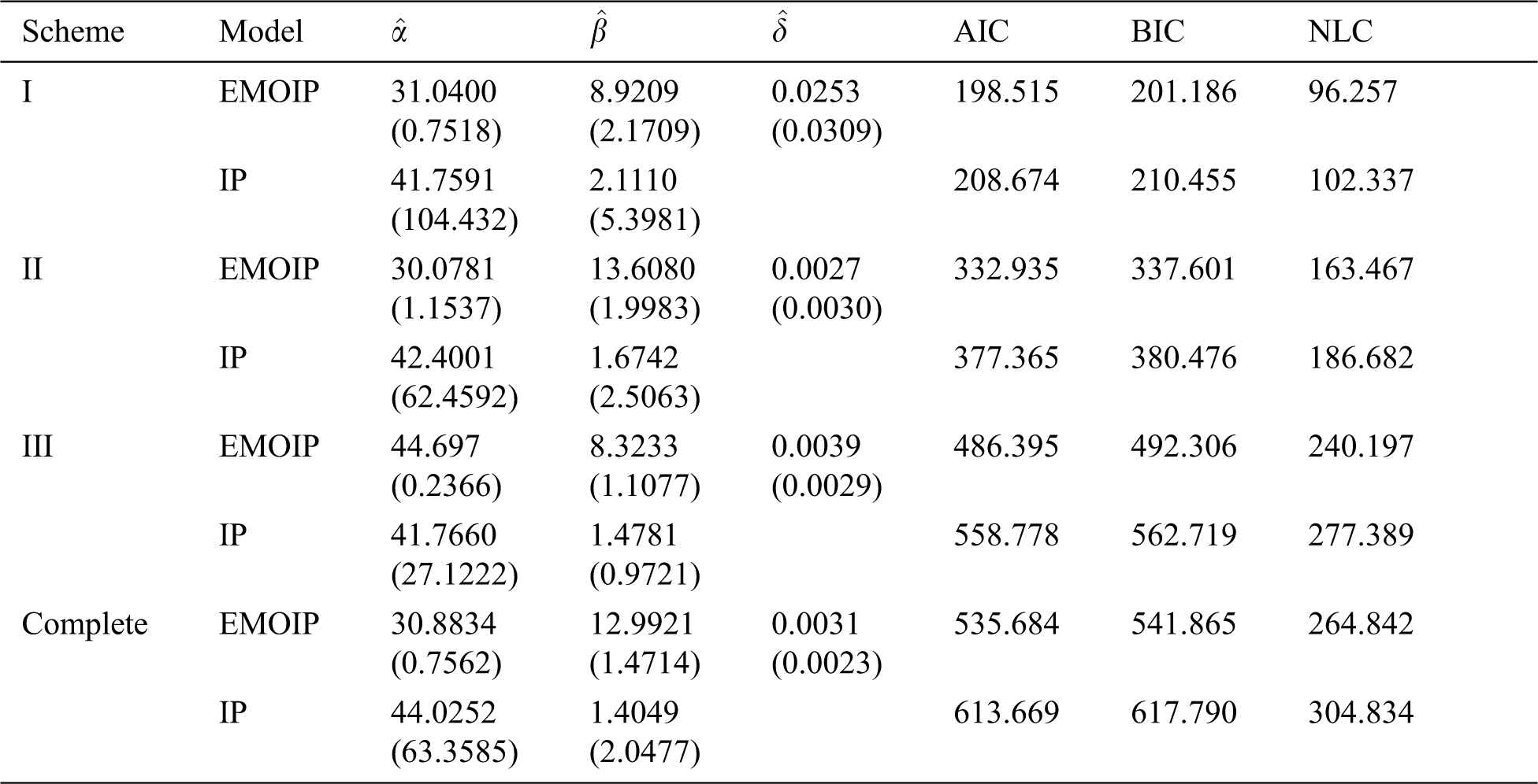
These methods will be compared using the Akaike’s information criterion (AIC), (BIC) Bayesian information criterion (BIC), and Negative log-likelihood criterion (NLC). The EMOIP and IP distributions are fitted to the given data set under the considered schemes.

The ML estimates of the parameters of the EMOIP and IP distributions along with their standard errors (SEs), AIC, BIC, and NLC were reported in Tabs. 13 and 14 for type-I and type-II censoring schemes, respectively. It is shown that the EMOIP provides a closer fit under the two types of censoring for all considered setups than the IP model.

Table 13: ML estimates, SEs, AIC, BIC and NLC of the EMOIP and IP distributions under type-I censored insurance data

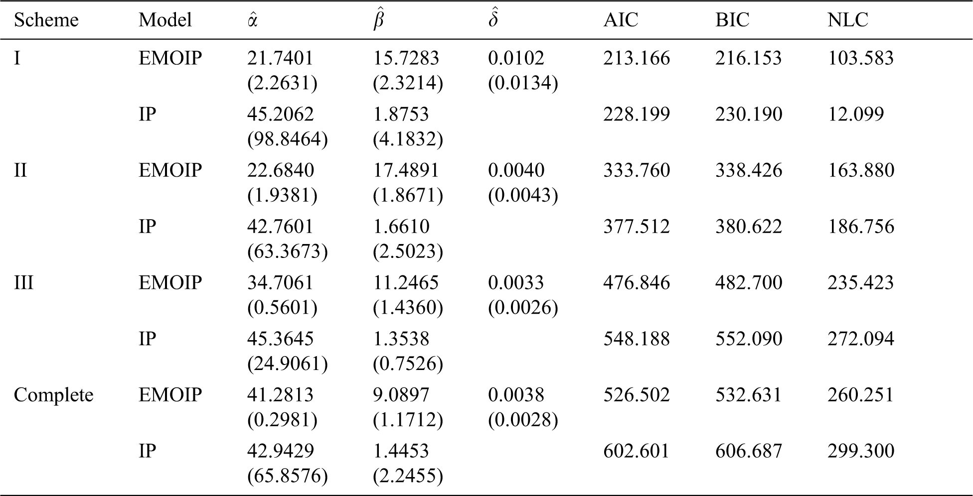
Table 14: ML estimates, SEs, AIC, BIC and NLC of the EMOIP and IP distributions under type-II censored insurance data

5  Concluding Remarks

In this paper, the Extended Marshall-Olkin Inverse Pareto (EMOIP) parameters are estimated using five classical estimation methods from complete samples, including the maximum likelihood, percentiles, least squares, maximum product spacings, and weighted least-squares. Furthermore, the EMOIP parameters are also estimated using the maximum likelihood estimation under type-I and type-II censored samples. Monte Carlo simulations are conducted to compare and explore the performance of the different estimators of the EMOIP parameters under complete and censored samples. Based on our study, the maximum likelihood is the best performing method in terms of its mean squared errors. We conduct another Monte Carlo simulation study to calculate the maximum likelihood estimators for the model parameters under type-I and type-II censoring schemes. Finally, we analyze a real data set to validate our results.

Availability of Data and Materials: The data sets used in this paper are provided within the main body of the manuscript.

Funding Statement: The authors received no specific funding for this study.

Conflicts of Interest: The authors declare that they have no conflicts of interest to report regarding the present study.

This work is licensed under a Creative Commons Attribution 4.0 International License, which permits unrestricted use, distribution, and reproduction in any medium, provided the original work is properly cited.