DOI:10.32604/iasc.2021.01000
| Intelligent Automation & Soft Computing DOI:10.32604/iasc.2021.01000 | |
| Article |
SVSF-Based Robust UGV/UAV Control/Tracking Architecture in Disturbed Environment
1Ecole Militaire Polytechnique, Algiers, Algeria
2Centre de Développement des Technologies Avancées, Algiers, Algeria
*Corresponding Author: Abdelatif Oussar. Email: oussarabdelatif@gmail.com
Received: 04 December 2019; Accepted: 03 July 2020
Abstract: This paper presents the design of a robust architecture for the tracking of an unmanned ground vehicle (UGV) by an unmanned aerial vehicle (UAV). To enhance the robustness of the ground vehicle in the face of external disturbances and handle the non-linearities due to inputs saturation, an integral sliding mode controller was designed for the task of trajectory tracking. Stabilization of the aerial vehicle is achieved using an integral-backstepping solution. Estimation of the relative position between the two agents was solved using two approaches: the first solution (optimal) is based on a Kalman filter (KF) the second solution (robust) uses a smooth variable structure filter (SVSF). Simulations results, based on the full non-linear model of the two agents are presented in order to evaluate the performance and robustness of the proposed tracking architecture.
Keywords: UGV/UAV tracking; integral sliding mode controller; trajectory tracking; integral-backstepping controller; Kalman filter; robust smooth variable structure filter
Nomenclature
| | Coordinates of UGV reference trajectory |
| | UGV desired control inputs |
| | UGV actual coordinates |
| | UGV control inputs |
| | Uncertainties on |
| | Radius of UGV wheels |
| | The distance between the two driving wheels |
| | Angular velocity of the two driving wheels |
| | Tracking errors |
| | Tracking errors expressed in the UGV frame |
| | Nominal and discontinuous part of the ISMC respectively |
| | The bounds of the UGV controls |
| | Sliding surface |
| | State vector describing the UGV motion |
| | Sampling period |
| | Random process noise |
| | The measurements of the UGV position |
| | Random measurement noise |
| | Quadrotor position and orientation |
| | Quadrotor control inputs |
| | Quadrotor virtual control inputs |
Unmanned aerial/ground cooperation is increasingly attracting the attention of researchers. This is essentially due to the complementary skills provided by each type to overcome the specific limitations of each other. UGVs offer a higher payload and stronger calculation capabilities, while UAVs provide faster dynamics, and add a local coverage for the unseen areas from an aerial view [1]. Indeed, deployment of integrated multi-robot team consisting of heterogeneous robots provides advantages compared to strict homogeneous compositions. One of the attractive scenarios for multi-agent system is the tracking of a ground target using an unmanned aerial vehicle [2]. This allows performing important tasks like surveillance of convoys, reconnaissance, and intelligence missions [3]. Tracking ground targets is more difficult than aerial ones due to the topographic variations that can influence a target’s motion patterns and obscurity to observation [4].
Many results related to this topic have been presented in the last few years. A circular pattern navigation algorithm for autonomous target tracking was presented in Rafi et al. [5] and Wise et al. [6], showing a good performance in simulation. Solutions based on partial information of the target state were presented in Peterson et al. [7], Summers et al. [8] and Kim et al. [9]. Observers, adaptive control, and extended Kalman filtering were used in this works for estimating the full target state. In Kim et al. [9] a non-linear model predictive controller was used to achieve the desired standoff configuration for an accelerating target. Quintero et al. [10] presented an output-feedback model predictive control with moving horizon estimation for target tracking by UAV, showing a good robustness.
Other works dealt with trajectory acquisition from video cameras, using particle filters for target estimation from non-stabilised cameras [11]. Multiple target tracking was achieved using Joint Probabilistic Data Association Filter (JPDAF) in the presence of unreliable target identification [12]. If a model for the object’s motion is known, an observer can be used to estimate the object’s velocity [13]. The recent work [14] covered one of the most important applications of estimation theory, namely, multi-target tracking, and included a thorough treatment of multisensor fusion and multiple hypothesis tracking, attribute-aided tracking, unresolved targets, sensor management, etc.
Air-ground collaborative systems find their applications in several fields. Authors in [15–21] present significant studies on Intelligence Surveillance and Reconnaissance (ISR) missions including both aerial and terrestrial vehicles. On the other hand, object tracking, path planning and localization are the others missions where this UAV/UGV cooperation is beneficial. We quote here some noteworthy studies [22–26] related with UAV/UGV systems collaborating to perform the above-mentioned tasks. As important part of this air-ground cooperation, many works have focused on “formation control” [27–29]. However, such hybrid UAV/UGV architecture can combine their tasks to achieve more complex missions [30–32].
More recently many studies have been made proposing new approaches to path planning for heterogeneous cooperating team (Air-ground Coordination). In Yulong et al. [33], Dubins path planning combined with Traveling Salesman problem was proposed to find the shortest route. A Quaternion based control for circular UAV trajectory tracking, following a ground vehicle was proposed in Abaunza et al. [34].
Guastella et al. [35] designed a global path planning strategy for a UGV from aerial elevation maps for disaster response. Peterson et al. [36] the authors present a collaborative UAV/UGV system to online aerial terrain mapping to inform the ground vehicle’s path planning in real time.
This kind of system can have practical applications for search and rescue missions. Some recent projects such as ICARUS [37] and ANKommEn [38] aims to develop a platform using multiple UAV and UGV for exploration of disaster scenarios for the detection of survivors and to provide maps in order to assist in maximizing the efficiency of Search and Rescue (SAR) operations.
In this paper, we first focus on the modeling and robust control of the two heterogeneous robots constituting the cooperative system. The second part covers the tracking problem of the ground agent by the UAV taking into account the dynamics of the aerial agent and the kinematics of the UGV. Since direct measurements are tainted with noise, it is essential to integrate an estimation filter allowing the prediction and estimation of the state of the ground target. We tested two estimation algorithms: the standard Kalman filter and the smooth variable structure filter.
The main contribution of this paper is the design of a new robust architecture for the tracking of an UGV by an UAV in order to deal with external disturbances and model uncertainties. To achieve this goal, the stabilization of the UAV is performed based on the integral-backstepping control approach while an integral sliding mode controller was designed for trajectory tracking. In addition, a comparative study of the proposed approaches for estimating the relative position between the two agents (UGV and UAV), is accomplished, illustrating the advantages of the proposed architecture.
The rest of this paper is organized as follows: in Section 2, the kinematic model of the UGV is presented and an integral sliding mode controller is designed in order to control the UGV motion. Section 3 provides the dynamic model of the UAV (quadrotor) together with the proposed control law based on the integral-backstepping approach. Section 4 presents the tracking algorithms used to estimate the state of the ground vehicle. In order to evaluate the proposed control and tracking architecture, simulation results with different scenarios are presented in Section 5.
2 UGV Modelling, Control and Trajectory Tracking
2.1 Formulation of the Trajectory Tracking Problem
We assume that the reference trajectory, generated by the motion planning algorithm, fulfils the following model:
where
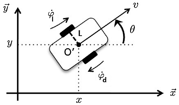
Figure 1: Unicycle-type mobile robot
It is obvious that the real controls
where the linear and angular velocities,
parameter
The objective of trajectory tracking is to asymptotically stabilize the tracking errors
Transforming the tracking errors expressed in the inertial frame to the robot frame, the error coordinates can be denoted as follows:
Thus, the tracking-error model is represented by the following equation:
where
2.2 Integral Sliding Mode Controller Design
Sliding Mode Control (SMC) is widely used in the control of different type of systems, such as wheeled mobile robot [40], five DOF redundant robot [41], PH process in stirred tanks [42], tunnel bow thrusters [43] or for other purpose such as multi-sensors data fusion [44]. In this part, we propose to enhance the SMC with the integral action, to improve its disturbances rejection. This controller is then applied to our UGV system.
For system Eq. (5), the control law is defined as follows:
The first part of the control design is to find a saturated control law
The positive parameters
For the ISMC part
where
The variable
with
In order to reduce the chattering phenomena, the sign function is replaced by:
Remark 1: The trajectory evolves on the manifold
2.3 Stability Analysis of the Smooth ISMC
Let us study the effect of the approximation of the sign function by tanh on global stability.
Lemma 1. [48] For every given scalar x and positive scalar
Proof of Lemma 1. According to the definition of tanh function, we have:
Since
Therefore
And
Proof of stability. Consider the following Lyapunov function candidate:
The discontinuous control term must satisfy the condition
According to Lemma 1, the above condition is satisfied if:
with
Therefore, according to LaSalle’s theorem, the control system with the smoothed ISMC is asymptotically stable in the sense of Lyapunov.
2.4 Tracking Algorithm based on Kalman Filter
Ground targets (UGVs) were always implicitly assumed to be non-manoeuvring and the noise statistics involved in the dynamics model/target observation (matrices
where:
and
and
where
As the measurement vector is the UGV position
The predicting and update equations for the Kalman filter are presented as follows:
Let us describe the Kalman filter parameters (
• For the initialization (
• The selection of matrices
The covariance matrix of the process noise (
3 Quadrotor Dynamics and Control
Our interest in such type of UAV (Fig. 2) is its hovering capability and high manoeuverability.
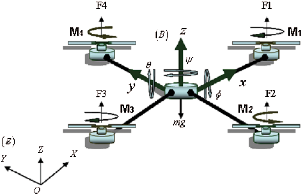
Figure 2: Quadrotor configuration
The dynamic models of the quadrotor are well studied. The details of the following Newton-Euler equations can be found in Refs. [50–53].
The control inputs of the UAV are defined as follows:
The description of the parameters used in this model is given in Tab. 1.
Table 1: Quadrotor parameters description

3.2 Backstepping Controller (BC) Design
In order to control the UAV a backstepping control scheme is used. The inner controller stabilizes the orientation angles in order to achieve a stable flight while the outer controller is responsible for the control of the position of UAV. Further the state vector of the UAV is defined as follows:
Thus we obtain the following equations:
with
The following Lyapunov functions are used:
with
The application of the backstepping technique [50] and [54] on the quadrotor state model give the following control inputs:
with
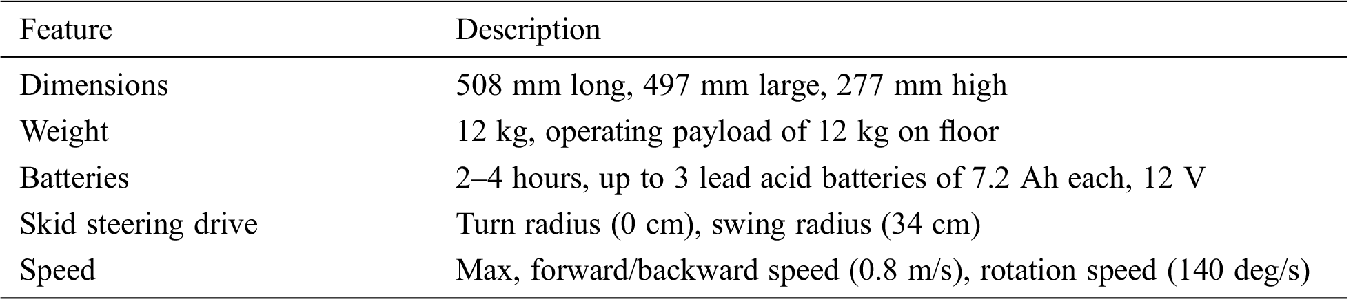
The simulation results are obtained based on the following realistic parameters of quadrotor in Tab. 2 and characteristics of Pioneer 3-AT mobile robot in Tab. 3.
Table 2: Quadrotor general parameters [50]
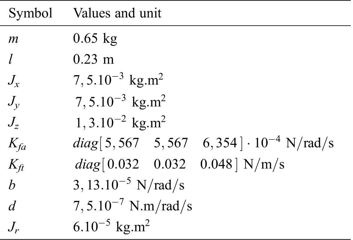
Table 3: Characteristics of the Pioneer 3-AT
In this first simulations set, we aim to evaluate the ISMC controller of the ground agent (UGV), thus the first tracking approach based on the Kalman filter and the backstepping control of the quadrotor.
In this context of the ground agent tracking by a UAV, and in order to get closer to reality, several scenarios are considered as follows.
• The initial conditions of the UGV:
• The initial conditions of the quadrotor:
• The control inputs of the quadrotor are bounded as follows:
• The initial parameters of the Kalman estimator are given as follows:
Scenario 1: The quadrotor may be affected by external disturbances such as wind. Several models of wind are proposed in Gawronski [55]. In our work, we assume that the wind has caused the same acceleration intensity on all axes
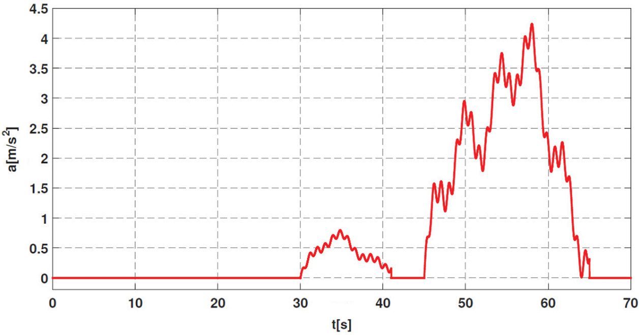
Figure 3: Time evolution of wind acceleration
• Scenario 2: This scenario is designed to evaluate the robustness of the control system with respect to modelling errors and measurement noises. In terms of parametric uncertainty, we assume that the elements of the inertia matrix
As for the measurement noises, an additive Gaussian white noise with the density
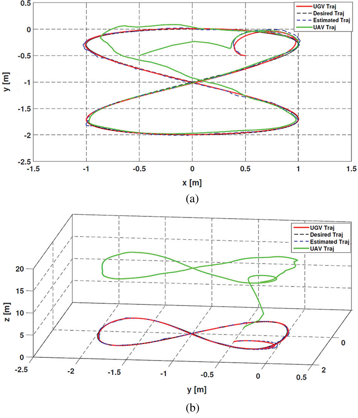
Figure 4: Tracking of UGV by the quadrotor in the presence of wind: (a) 2D, (b) 3D
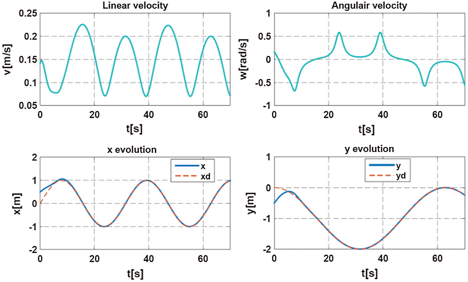
Figure 5: Evolution in time of the mobile robot position and control inputs
In the presence of wind gusts (Fig. 3) and as shown in Fig. 4, the quadrotor tracks the UGV that traveled Eight trajectory using the ISMC controller. By looking at Figs. 5 and 6, it can be noticed that the ISMC allows the robot to follow the set point correctly according to the two axes
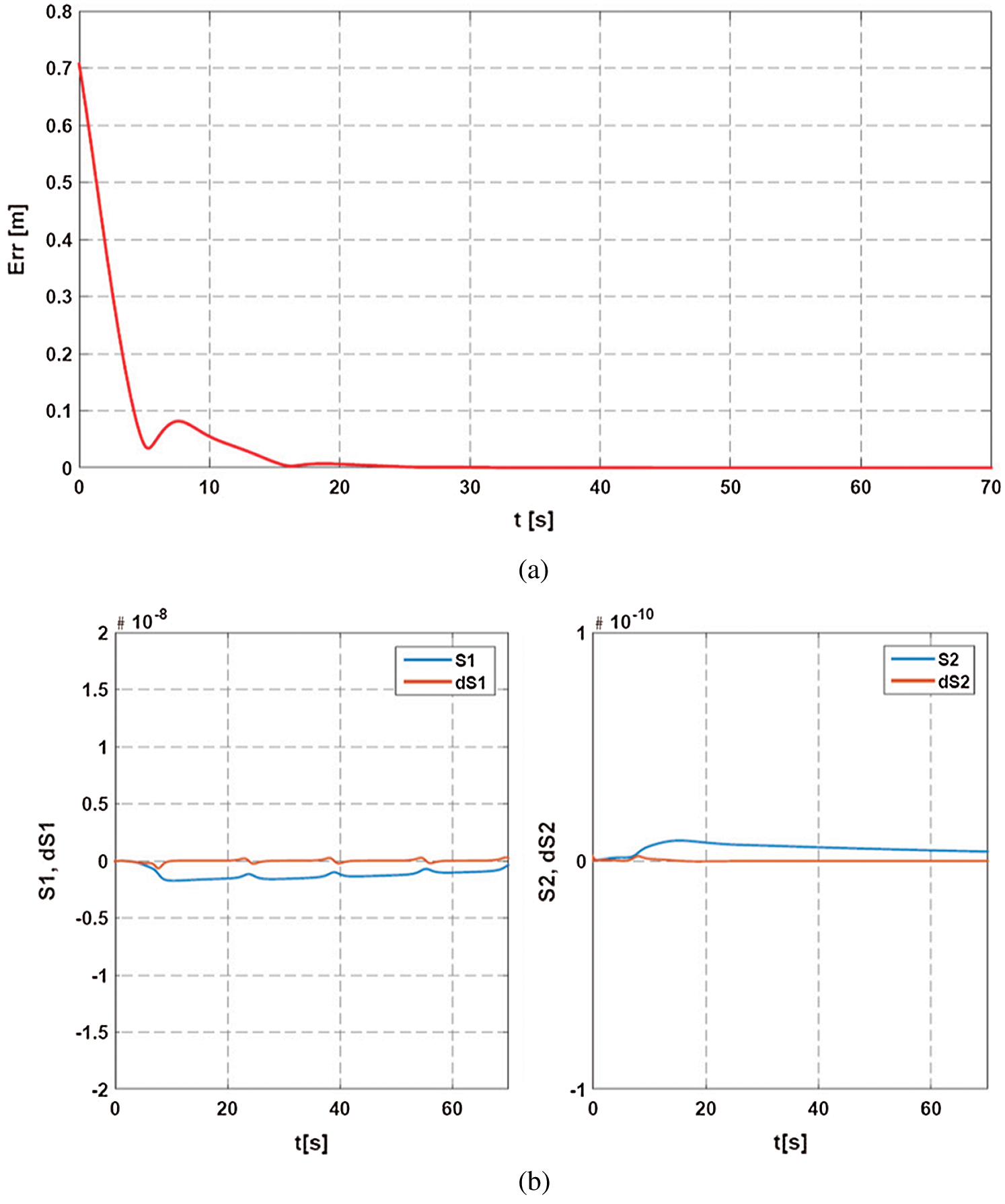
Figure 6: Evolution in time of: (a) Tracking error (b) The sliding surfaces
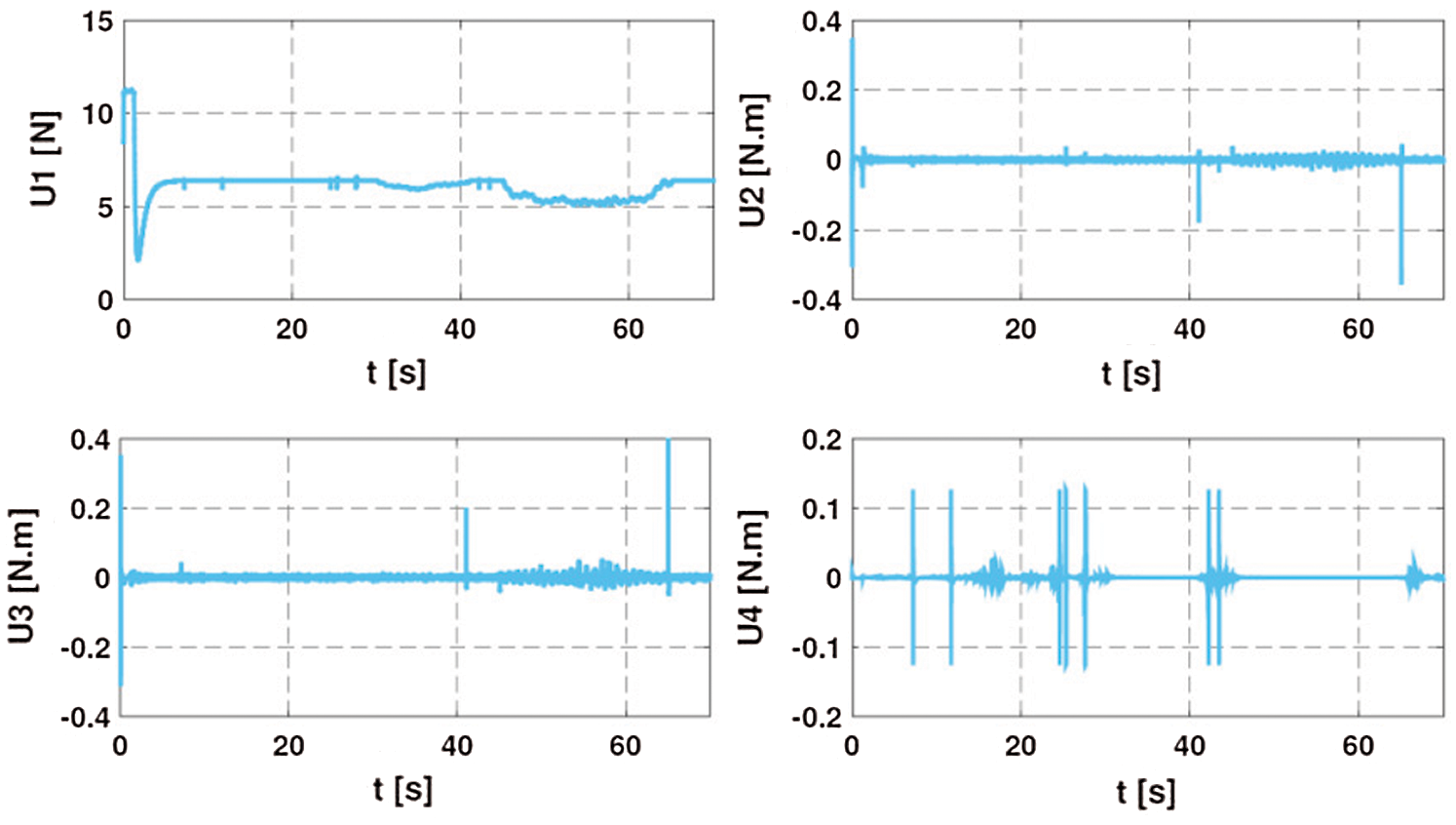
Figure 7: Control inputs of the quadrotor in the presence of wind disturbance (scenario 1)
As for scenario 1, even with the existence of parametric uncertainties and measurement noises, the quadrotor succeeds in tracking the mobile robot with small fluctuations in its tracking trajectory (Fig. 9). The tracking error along

Figure 8: Evolution of the quadrotor: (a) Translation (x,y,z) (b) Orientation angles (scenario 1)
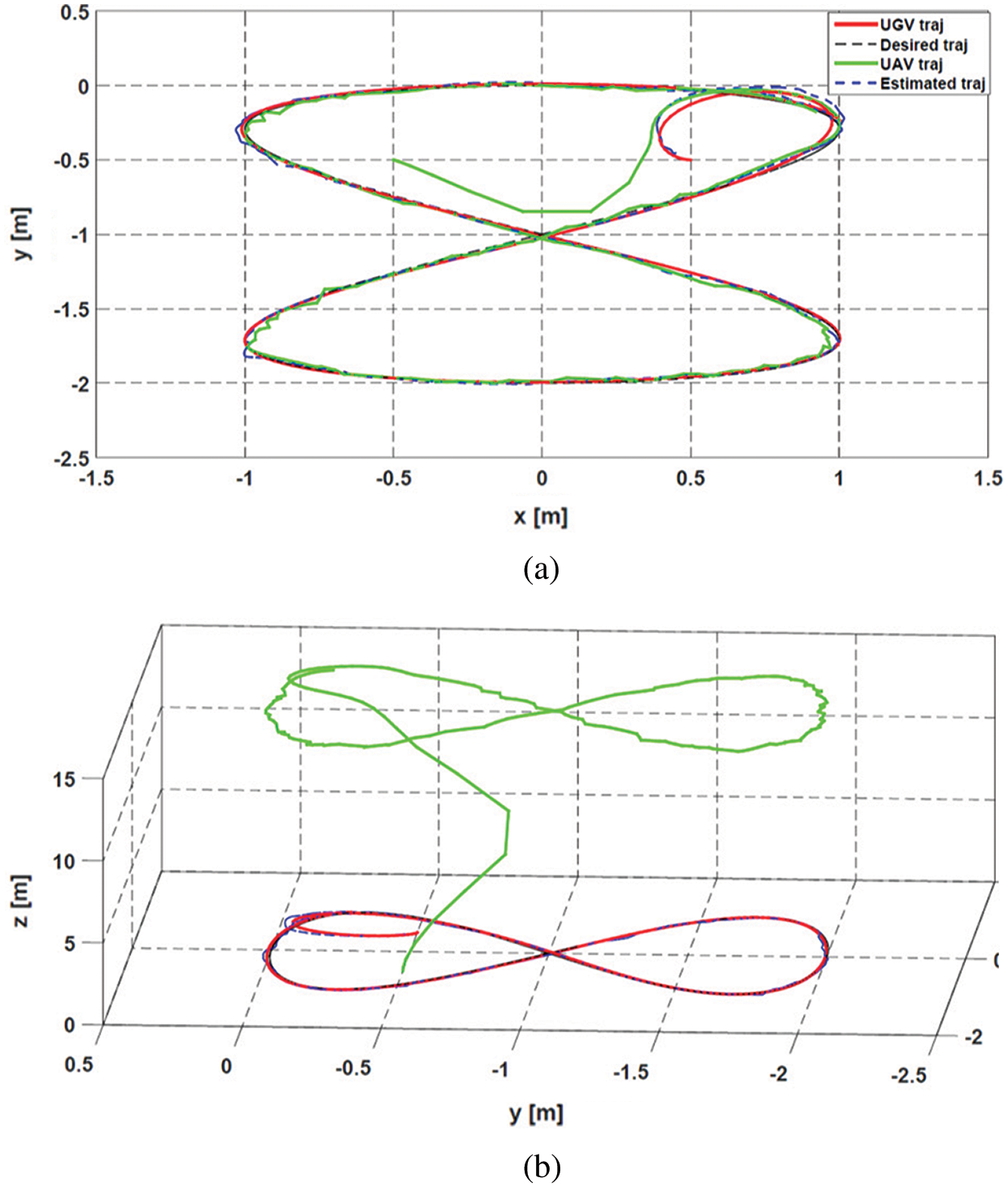
Figure 9: Tracking of UGV by the quadrotor with parametric uncertainties and measurement noise: (a) 2D, (b) 3D
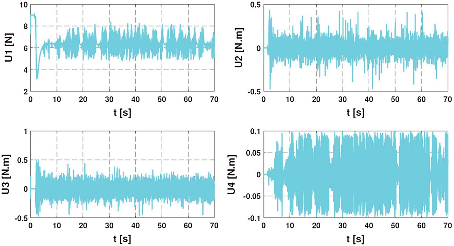
Figure 10: The control inputs of the quadrotor (scenario 2)
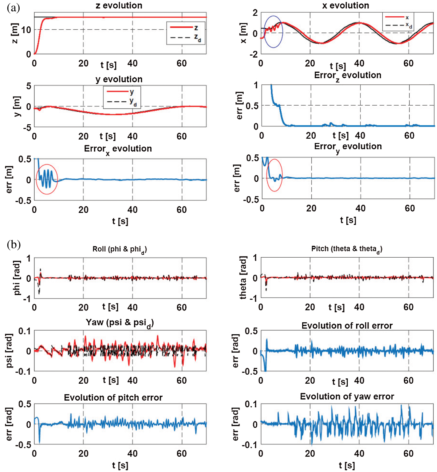
Figure 11: Evolution of the quadrotor: (a) Translation (x,y,z) (b) Orientation angles (scenario 2)
4 Robust Control/Tracking Architecture
4.1 Robust Tracking algorithm based on SVSF
One of the major challenges for the tracking algorithm is the uncertainty in the motion of UGV. This uncertainty refers to the fact that a precise dynamic model of the movement is not available at the level of the tracking algorithm [57,58]. However, the Kalman filter (KF) can only achieve a good performance (optimal solution) under the assumption that the complete and exact information of the process model and the noise distribution are to be known as a prior. In practice, state and observation models are often poorly known, or contain uncertain parameters, and the statistical properties of noise (state and observation) are also poorly known, coming to the optimality of the solution obtained. Therefore, to improve our tracking algorithm, and to overcome these limitations, we propose to use a new filter or estimator called Smooth Variable Structure Filter (SVSF) to process the tracking problem of a UGV [59,60].
The Smooth Variable Structure Filter is a relatively new estimating strategy proposed by Habibi in 2007 [61]. This strategy is based on the concepts of sliding mode control and the theory of systems with variable structure, outcome and similar design to variable structure filter (VSF) [62]. This filter is formulated in the predictive-correction format, and can be used for linear or non-linear systems. It uses a correction gain simpler than the one used by the VSF. The SVSF is introduced to provide more stability and robustness to the estimation process. This technique is generally used for the estimation of states and parameters of dynamic systems [63], the prediction and diagnosis of defects in systems [64] and targets tracking problems [59,60,65].
To formulate the tracking problem, we use the same model that has been described in detail by the two Eqs. (15) and (18).
The SVSF estimation method is described by the following series of equations. Note that this formulation includes state error covariance equations as presented in Gadsden et al. [66], which was not originally presented in the standard SVSF form [61]. The prediction stage is similar to the KF; its steps are as follows:
- Initialization
- Prediction
where
then, pretest measurement error is calculated by the following equation:
- Update
For the state estimate, the SVSF correction gain is calculated by MacArthur et al. [22] and Phan et al. [31]:
where
The form of saturation used in Eq. (35) is defined as follows:
The gain is used to update the predicted state as follows:
The covariance associated with the state updates is then calculated as follows:
Thus, the estimated measurement and the corresponding empirical measurement error are calculated as follows:
Two critical variables in this process are the pretest and empirical measurements (output) error estimates, defined by Eqs. (34) and (40). It shall be noted that Eq. (40) is the empirical measurement error estimates from the previous time step, and is used only in the gain calculation.
The selection of the smoothing boundary layer width vector
4.2 Integral-Backstepping Controller (IBC)
The backstepping control cannot ensure the favorable tracking performance of the quadrotor if unpredictable disturbances from the unknown external disturbance, modeling errors, as well as measurement noise occur. In order to improve these performances and consequently the robustness, we propose to combine the conventional PID with the backstepping control. This will allow for integral backstepping. However, this control technique has been proposed in several research studies [50,52,67,68,69], which demonstrated that the integral backstepping controller allows rejection of external disturbances and is robust to parametric uncertainties.
The application of the integral backstepping control on the quadrotor state model gives the following control inputs:
Such as:
and the Lyapunov functions take the following form:
For the selection of the controller parameters, we have used an approach based on PSO (Particle Swarm Optimization) optimization method, more details can be found in Yacef et al. [70].
After explaining and presenting the various tracking algorithms (KF and SVSF), showing the principle and the mathematical development. Their estimation accuracy and robustness to different types of noise will be evaluated. The root mean square error (RMSE) of the different results is calculated for different scenarios.
Scenario 3: In this scenario, the favorable conditions for the Kalman filter will be placed, by applying on the states and on the obtained measurements decorrelated centered noises as covariance matrix:
The
The expression of RMSE on the estimate is given by the following equation:
The expression of RMSE on the estimation of the position of the mobile robot is given by the following equation:
The implementation results under Matlab are shown in Fig. 12 for the two algorithms. In order to evaluate the estimation accuracy, we calculated the RMSE on the estimate. Tab. 4 shows the results obtained.
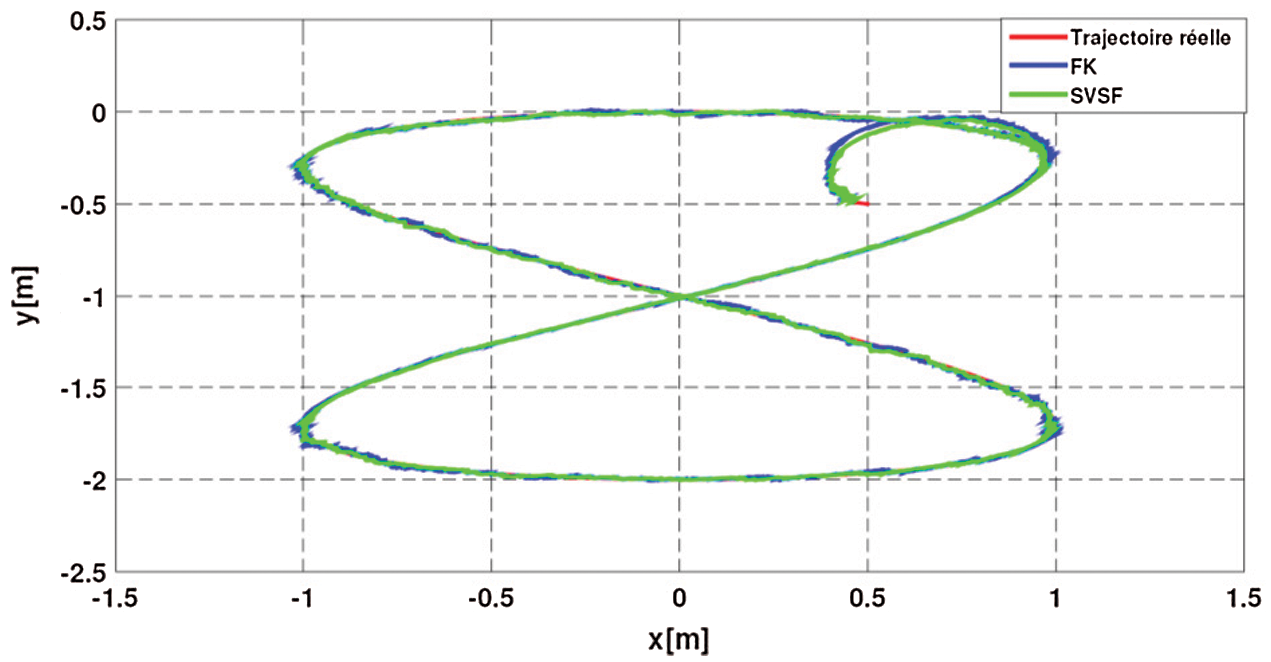
Figure 12: The trajectories estimated by the different algorithms
Table 4: Comparison of the different estimation algorithms with RMSE for Scenario 3
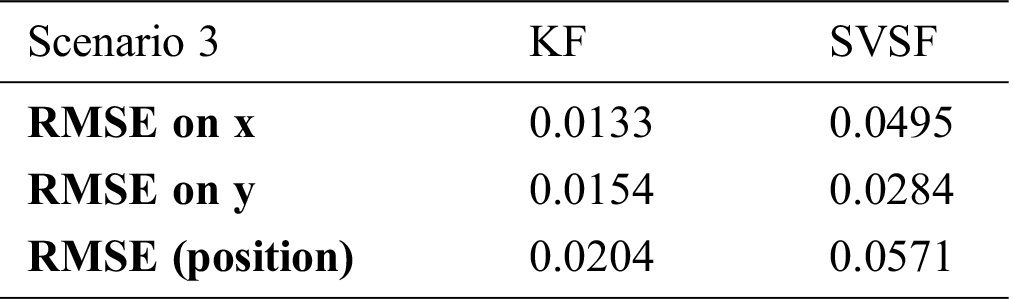
It was found that the values of RMSE of the Kalman filter are lower than those of the SVSF. In this scenario we deduced that the estimation of the trajectory of the UGV by the KF is more accurate in comparison with the SVSF.
Scenario 4: In this scenario, unfavorable conditions for the Kalman filter will be considered, in order to show the efficiency, robustness and superiority of the SVSF with respect to the KF, when the initial conditions are poorly chosen (the initial conditions are increased by a factor of 10), so that noises on states and measurements are Gaussian, correlated, non-centered:
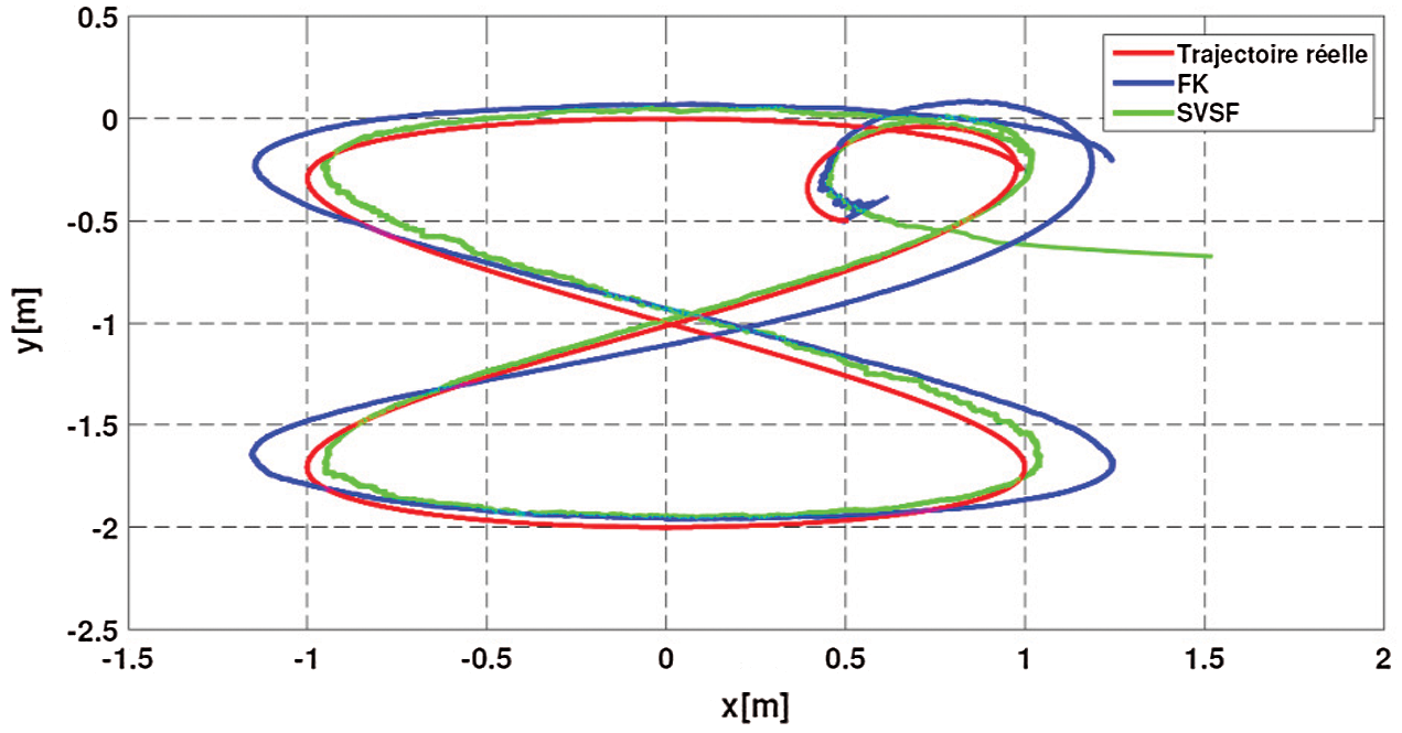
Figure 13: The estimated trajectories by different algorithms
Fig. 13 shows the estimated trajectories of the UGV and the RMSE are given in Tab. 5.
Table 5: Comparison of the different estimation algorithms with RMSE for Scenario 4
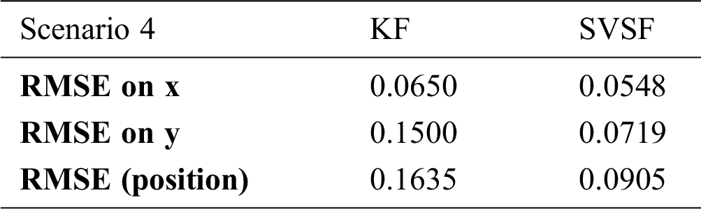
It was found that the values of
5.2 Robust Ground Agent Tracking using SVSF and IBC of UAV
In order to evaluate the performance of this architecture, we mainly integrate in this case two scenarios 1 and 2 described above and based on the results of estimation of the SVSF to carry out missions of tracking a ground agent. The initial conditions and constraints are the same. The initial parameters of the SVSF estimator are given in Eqs. (44) and (45).
From the results of Fig. 14, it is clear that the IBC control is more efficient. This control (Fig. 15) reduces tracking errors. For example, in Scenario 1, we obtained 0.08 m in
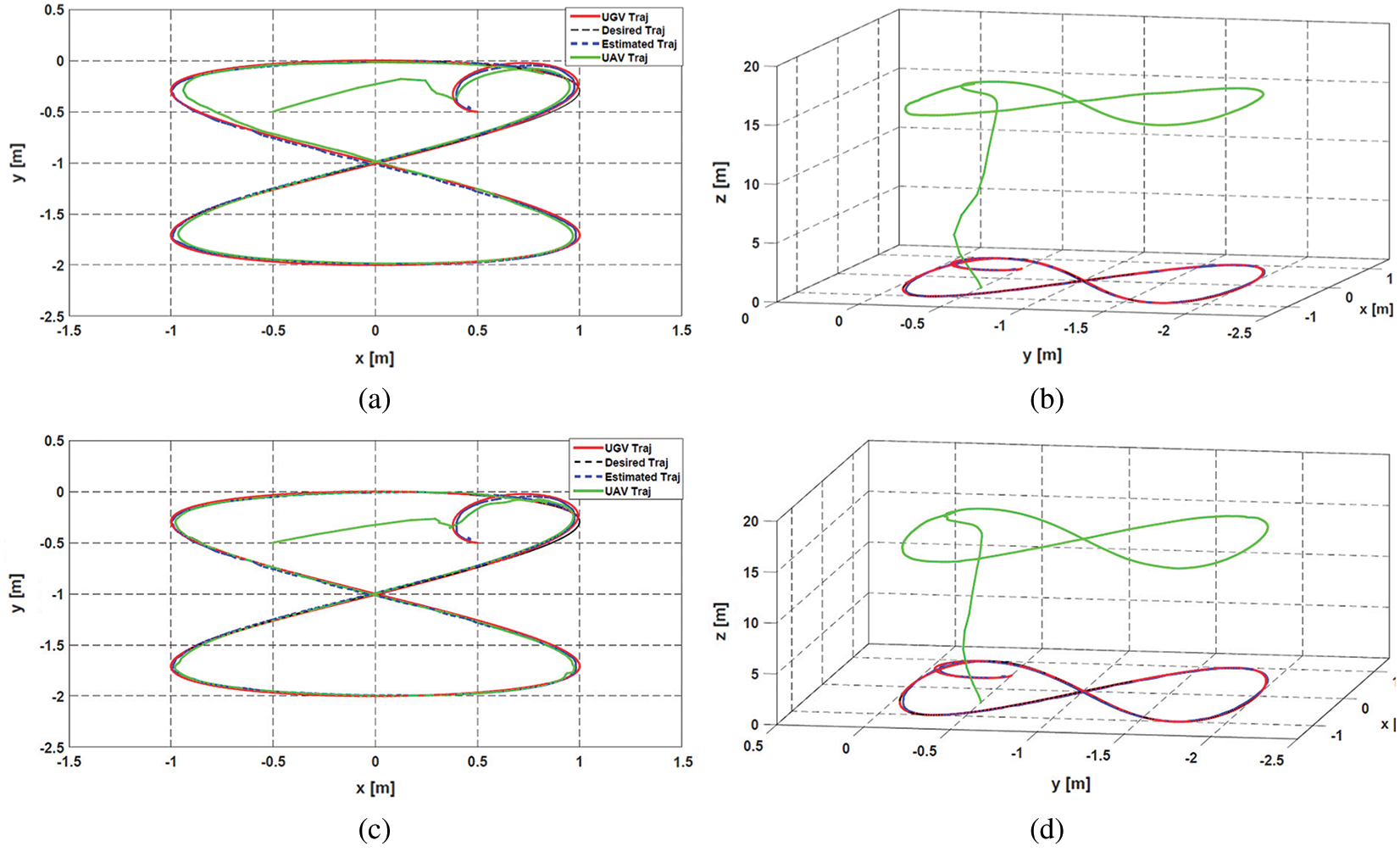
Figure 14: Tracking of UGV by UAV using SVSF and the IBC: scenario 1 ((a) 2D, (b) 3D), scenario 2 ((c) 2D, (d) 3D)
Thus, it can be deduced that the IBC makes it possible to obtain a better robustness with respect to the parametric uncertainties and a better rejection of the external disturbances with respect to the BC.
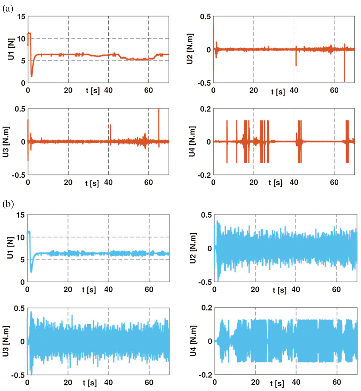
Figure 15: Integral backstepping control inputs of the quadrotor for different scenarios: (a) scenario 1, (b) scenario 2
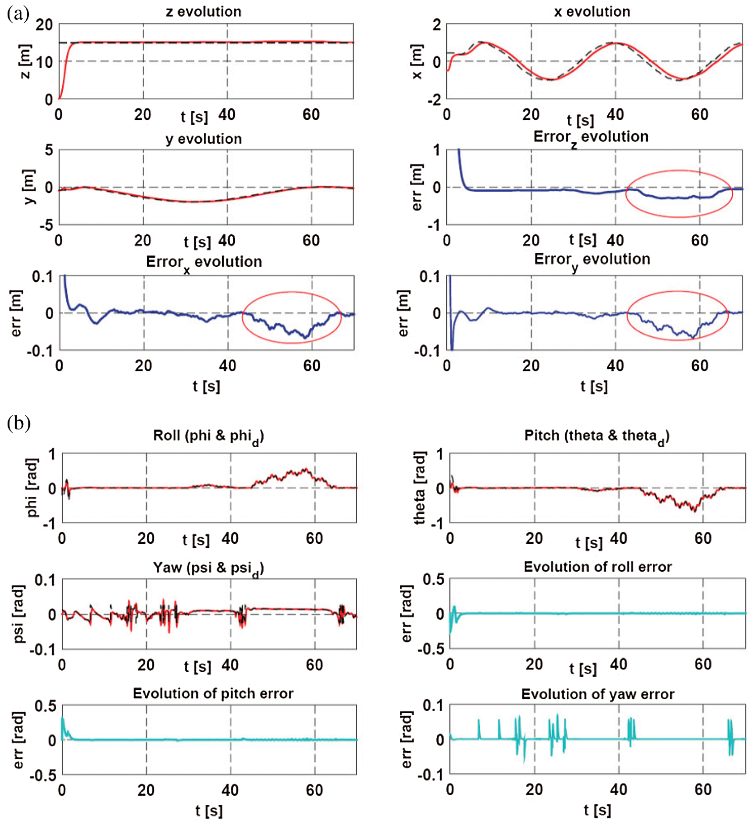
Figure 16: Evolution of the translation (x, y, z) and the angles of orientation of the quadrotor with wind disturbance respectively (a) and (b)
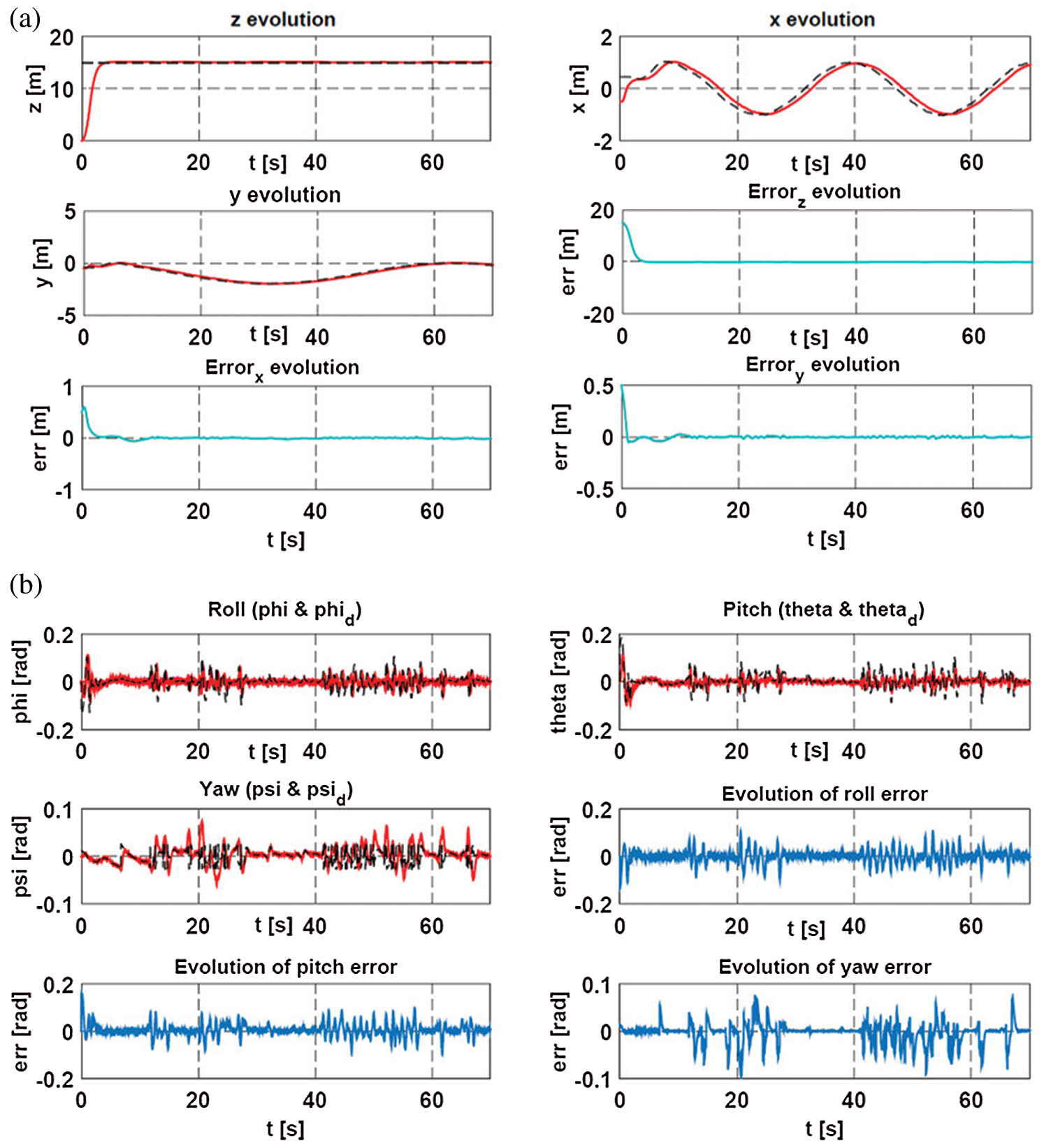
Figure 17: Evolution of the translation (x, y, z) and the angles of orientation of the quadrotor with parametric uncertainties and measurement noises respectively (a) and (b)
This paper proposed a robust control and tracking architecture in order to allow for an UAV to track an UGV in disturbed environment. The considered UGV is a Unicycle mobile robot. On one hand, the latter has been controlled based on the Integral Sliding Mode technique taking into account the kinematics constraints on the speed limitations. A tracking algorithm based on the Kalman filter was introduced in order to estimate the relative state of the UGV in a disturbed environment. On the other hand, a considered UAV type quadrotor and a backstepping controller is designed to stabilize this UAV. A first set of simulations was performed by considering several scenarios. The simulation results of this tracking architecture have shown limited robustness with respect to external disturbances, modeling errors and measurement noises.
In order to improve the performance of this architecture, the Kalman filter has been replaced by the Smooth Variable Structure Filter and the integral-backstepping controller was introduced in order to overcome the challenges of classical backstepping robustness. The stability of the synthesized control laws has been proved by the Lyapunov theory; which is necessary to achieve UGV/UAV cooperation architecture. The second set of simulations considering the proposed architecture has shown the improvement of robustness and accuracy of this architecture.
Current and future works concern the implementation of the proposed architecture and algorithms on a Pixhawk autopilot for UAV control and Raspberry Pi based vision module for automated UGV target visual detection, recognition and tracking.
Acknowledgement: We would like to thank the staff of the Ecole Militaire Polytechnique of Algiers, especially Doctor Oualid Araar, for the assistance afforded to perform this research.
Funding Statement: The authors received no specific funding for this study.
Conflicts of Interest: The authors declare that they have no conflicts of interest to report regarding this study.
1. E. H. C. Harik, F. Guinand, H. Pelvillain, F. Guérin and J. F. Brethé, “A decentralized interactive architecture for aerial and ground mobile robots cooperation,” in Proc. Int. Conf. on Control, Automation and Robotics, Singapore, pp. 37–43, 2015. [Google Scholar]
2. A. Ferrag, A. Oussar and M. Guiatni, “Robust coordinated motion planning for UGV/UAV agents in disturbed environment,” in Proc. 8th International Conference on Modelling, Identification and Control (ICMICAlgiers, pp. 472–477, 2016. [Google Scholar]
3. J. E. Gomez-Balderas, P. Castillo, J. A. Guerrero and R. Lozano, “Vision based tracking for a quadrotor using vanishing points,” Journal of Intelligent & Robotic Systems, vol. 65, no. 1–4, pp. 361–371, 2012. [Google Scholar]
4. C. C. Ke, J. G. Herrero and J. Llinas, “Comparison of techniques for ground target tracking,” in State University of New York At Buffalo Center Of Multisource Information Fusion, Rep. ADA400079, 2000. [Google Scholar]
5. F. Rafi, S. Khan, K. Shafiq and M. Shah, “Autonomous target following by unmanned aerial vehicles,” Unmanned Systems Technology VIII, vol. 6230, pp. 10–18, 2006. [Google Scholar]
6. R. Wise and R. Rysdyk, “UAV coordination for autonomous target tracking,” in Proc. AIAA Guidance, Navigation, and Control Conf. and Exhibit, Colorado, pp. 6453–6475, 2006. [Google Scholar]
7. C. Peterson and D. A. Paley, “Multivehicle coordination in an estimated time-varying flowfield,” Journal of Guidance, Control, and Dynamics, vol. 34, no. 1, pp. 177–191, 2011. [Google Scholar]
8. T. H. Summers, M. R. Akella and M. J. Mears, “Coordinated standoff tracking of moving targets: Control laws and information architectures,” Journal of Guidance, Control, and Dynamics, vol. 32, no. 1, pp. 56–69, 2009. [Google Scholar]
9. S. Kim, H. Oh and A. Tsourdos, “Nonlinear model predictive coordinated standoff tracking of a moving ground vehicle,” Journal of Guidance, Control, and Dynamics, vol. 36, no. 2, pp. 557–566, 2013. [Google Scholar]
10. S. A. P. Quintero, D. A. Copp and J. P. Hespanha, “Robust UAV coordination for target tracking using output-feedback model predictive control with moving horizon estimation,” in Proc. American Control Conf. (ACCChicago, pp. 3758–3764, 2015. [Google Scholar]
11. J. Lee, R. Huang, A. Vaughn, X. Xiao and J. K. Hedrick, “Strategies of path-planning for a UAV to track a ground vehicle,” in AINS Conf., Sengupta, 2003. [Google Scholar]
12. Y. Bar-Shalom, Tracking and data association. San Diego: Academic Press Professional, Inc., 1987. [Google Scholar]
13. B. K. Ghosh and E. P. Loucks, “A realization theory for perspective systems with applications to parameter estimation problems in machine vision,” IEEE Transactions on Automatic Control, vol. 41, no. 12, pp. 1706–1722, 1996. [Google Scholar]
14. Y. Bar-Shalom, P. K. Willett and X. Tian, Tracking and data fusion. Storrs: YBS publishing, 2011. [Google Scholar]
15. F. Capezio, A. Sgorbissa and R. Zaccaria, “GPS-based localization for a surveillance UGV in outdoor areas,” in Proc. the Fifth Int. Workshop on Robot Motion and Control (RoMoCo’05Dymaczewo, pp. 157–162, 2005. [Google Scholar]
16. C. C. Haddal and J. Gertler, Homeland security: Unmanned aerial vehicles and border surveillance. Library of Congress Washington DC Congressional Research Service, Rep. ADA524297, 2010. [Google Scholar]
17. C. Pippin, G. Gray, M. Matthews, D. Price, A. P. Hu et al., “The design of an air-ground research platform for cooperative surveillance,” Georgia Tech Research Institute. Tech. Rep. 112010, 2010. [Google Scholar]
18. A. M. Khaleghi, D. Xu, Z. Wang, M. Li, A. Lobos et al., “A DDDAMS-based planning and control framework for surveillance and crowd control via UAVs and UGVs,” Expert Systems with Applications, vol. 40, no. 18, pp. 7168–7183, 2013. [Google Scholar]
19. M. Saska, T. Krajnik and L. Pfeucil, “Cooperative μUAV-UGV autonomous indoor surveillance,” in Proc. 9th Int. Multi-Conf. on Systems, Signals and Devices (SSDChemnitz, pp. 1–6, 2012. [Google Scholar]
20. H. G. Tanner and D. K. Christodoulakis, “Cooperation between Aerial and Ground vehicle groups for Reconnaissance missions,” in Proc. of the 45th IEEE Conf. on Decision and Control, San Diego, CA, pp. 5918–5923, 2006. [Google Scholar]
21. B. Grocholsky, J. Keller and V. Kumar, “Cooperative air and ground surveillance,” IEEE Robotics & Automation Magazine, vol. 13, no. 3, pp. 16–25, 2006. [Google Scholar]
22. D. K. MacArthur and C. D. Crane, “Unmanned ground vehicle state estimation using an unmanned air vehicle,” in Proc. Int. Sym. on Computational Intelligence in Robotics and Automation, Jacksonville, FI, pp. 473–478, 2007. [Google Scholar]
23. S. Kanchanavally, R. Ordonez and J. Layne, “Mobile target tracking by networked uninhabited autonomous vehicles via hospitability maps,” in Proc. of the American Control Conf., Boston, MA, USA, pp. 5570–5575, 2004. [Google Scholar]
24. R. Madhavan, T. Hong and E. Messina, “Temporal range registration for unmanned ground and aerial vehicles,” Journal of Intelligent and Robotic Systems, vol. 44, no. 1, pp. 47–69, 2005. [Google Scholar]
25. U. Zengin and A. Dogan, “Real-time target tracking for autonomous UAVs in adversarial environments: A gradient search algorithm,” IEEE Transactions on Robotics, vol. 23, no. 2, pp. 294–307, 2007. [Google Scholar]
26. J. Y. Choi and S. G. Kim, “Collaborative tracking control of UAV-UGV,” International Journal of Mechanical, Aerospace, Industrial, Mechatronic and Manufacturing Engineering, vol. 6, no. 11, pp. 2487–2493, 2012. [Google Scholar]
27. S. Ulun and M. Unel, “Coordinated motion of UGVs and a UAV,” in Proc. IECON 39th Annual Conf. of the IEEE Industrial Electronics Society, Vienna, pp. 4079–4084, 2013. [Google Scholar]
28. M. Saska, V. Vonásek, T. Krajník and L. Přeučil, “Coordination and navigation of heterogeneous UAVs-UGVs teams localized by a hawk-eye approach,” in Proc. IEEE/RSJ Int. Conf. on Intelligent Robots and Systems, Vilamoura, pp. 2166–2171, 2012. [Google Scholar]
29. L. Barnes, R. Garcia, M. Fields and K. Valavanis, “Swarm formation control utilizing ground and aerial unmanned systems,” in Proc. IEEE/RSJ Int. Conf. on Intelligent Robots and Systems, Nice, pp. 4205–4205, 2008. [Google Scholar]
30. N. Rackliffe, H. A. Yanco and J. Casper, “Using geographic information systems (GIS) for UAV landings and UGV navigation,” in Proc. IEEE Conf. on Technologies for Practical Robot Applications, Woburn, MA, pp. 145–150, 2011. [Google Scholar]
31. C. Phan and H. H. T. Liu, “A cooperative UAV/UGV platform for wildfire detection and fighting,” in Proc. Asia Simulation Conf.—7th Int. Conf. on System Simulation and Scientific Computing, Beijing, pp. 494–498, 2008. [Google Scholar]
32. P. Tokekar, J. V. Hook and D. Mulla, “Sensor planning for a symbiotic UAV and UGV system for precision agriculture,” IEEE Transactions on Robotics, vol. 32, no. 6, pp. 1498–1511, 2016. [Google Scholar]
33. D. Yulong, X. Bin, C. Jie, F. Hao and Z. Yangguang, “Path planning of messenger UAV in air-ground coordination,” IFAC-PapersOnLine, vol. 50, no. 1, pp. 8045–8051, 2017. [Google Scholar]
34. H. Abaunza, E. Ibarra, P. Castillo and A. Victorino, “Quaternion based control for circular UAV trajectory tracking, following a ground vehicle: Real-time validation,” IFAC-PapersOnLine, vol. 50, no. 1, pp. 11453–11458, 2017. [Google Scholar]
35. D. C. Guastella, L. Cantelli, C. D. Melita and G. Muscato, “A global path planning strategy for a UGV from aerial elevation maps for disaster response,” in Proc. 9th Int. Conf. on Agents and Artificial Intelligence(ICAARTPorto, pp. 335–342, 2017. [Google Scholar]
36. J. Peterson, H. Chaudhry, K. Abdelatty and J. Bird, “Online aerial terrain mapping for ground robot navigation,” Sensors, vol. 18, no. 2, pp. 630–652, 2018. [Google Scholar]
37. S. Govindaraj, K. Chintamani and J. Gancet, “The ICARUS project—Command, control and intelligence (C2I),” in Proc. IEEE Int. Sym. on Safety, Security, and Rescue Robotics (SSRRLinkoping, pp. 1–4, 2013. [Google Scholar]
38. S. Batzdorfer, M. Bobbe, M. Becker, H. Harms and U. Bestmann, “Multisensor equipped UAV/UGV for automated exploration,” The International Archives of Photogrammetry, Remote Sensing and Spatial Information Sciences, vol. 42, pp. 33–41, 2017. [Google Scholar]
39. M. Defoort, J. Palos, A. Kokosy, T. Floquet, W. Perruquetti et al., “Experimental motion planning and control for an autonomous nonholonomic mobile robot,” in Proc. IEEE Int. Conf. on Robotics and Automation, Roma, pp. 2221–2226, 2007. [Google Scholar]
40. M. Asif, A. Y. Memon and M. J. Khan, “Output feedback control for trajectory tracking of wheeled mobile robot,” Intelligent Automation & Soft Computing, vol. 22, no. 1, pp. 75–87, 2015. [Google Scholar]
41. J. A. Ruz-Hernandez, E. N. Sanchez and M. Saad, “Real-time decentralized neural control for a five Dof redundant robot,” Intelligent Automation & Soft Computing, vol. 19, no. 1, pp. 23–37, 2013. [Google Scholar]
42. L. E. Zárate and P. Resende, “Fuzzy sliding mode controller for a PH process in stirred tanks,” Intelligent Automation & Soft Computing, vol. 18, no. 4, pp. 349–367, 2012. [Google Scholar]
43. M. H. Casado and F. J. Velasco, “Thruster control based on the shunt DC motors for a precise positioning of the marine vehicles,” Intelligent Automation & Soft Computing, vol. 15, no. 3, pp. 425–438, 2009. [Google Scholar]
44. S. Bogosyan, “A sliding mode based neural network for data fusion and estimation using multiple sensors,” Intelligent Automation & Soft Computing, vol. 17, no. 4, pp. 477–493, 2011. [Google Scholar]
45. Z. P. Jiang, E. Lefeber and H. Nijmeijer, “Saturated stabilization and tracking of a nonholonomic mobile robot,” Systems & Control Letters, vol. 42, no. 5, pp. 327–332, 2001. [Google Scholar]
46. M. Defoort, T. Floquet and A. Kokosy, “Integral sliding mode control for trajectory tracking of a unicycle type mobile robot,” Integrated Computer-Aided Engineering, vol. 13, no. 3, pp. 277–288, Jul. 2006. [Google Scholar]
47. R. Abbas and Q. Wu, “Formation tracking for multiple quadrotor based on sliding mode and fixed communication topology,” in Proc. 5th Int. Conf. on Intelligent Human-Machine Systems and Cybernetics, Hangzhou, pp. 233–238, 2013. [Google Scholar]
48. M. P. Aghababa and M. E. Akbari, “A chattering-free robust adaptive sliding mode controller for synchronization of two different chaotic systems with unknown uncertainties and external disturbances,” Applied Mathematics and Computation, vol. 218, no. 9, pp. 5757–5768, 2012. [Google Scholar]
49. X. R. Li and V. P. Jilkov, “Survey of maneuvering target tracking: Dynamic models,” Signal and Data Processing of Small Targets, vol. 4048, pp. 212–236, 2000. [Google Scholar]
50. S. Bouabdallah, “Design and control of quadrotors with application to autonomous flying,” Ph.D dissertation. École Polytechnique Fédérale de Lausanne (EPFLLausanne, 2007. [Google Scholar]
51. R. Mahony, V. Kumar and P. Corke, “Multirotor aerial vehicles: Modeling, estimation, and control of quadrotor,” IEEE Robotics & Automation Magazine, vol. 19, no. 3, pp. 20–32, 2012. [Google Scholar]
52. H. Khebbache, B. Sait, Naâmane Bounar et al., “Robust stabilization of a quadrotor UAV in presence of actuator and sensor faults,” International Journal of Instrumentation and Control Systems, vol. 2, no. 2, pp. 53–67, 2012. [Google Scholar]
53. F. Yacef, O. Bouhali, M. Hamerlain and N. Rizoug, “Observer-based adaptive fuzzy backstepping tracking control of quadrotor unmanned aerial vehicle powered by Li-ion battery,” Journal of Intelligent & Robotic Systems, vol. 84, no. 1–4, pp. 179–197, 2016. [Google Scholar]
54. E. C. Suiçmez, “Trajectory tracking of a quadrotor unmanned aerial vehicle (UAV) via attitude and position control,” Ph.D. dissertation. Middle East Technical University, Ankara, 2014. [Google Scholar]
55. W. Gawronski, “Three models of wind-gust disturbances for the analysis of antenna pointing accuracy,” Jet Propulsion Laboratory, California Institute of Technology, vol. 42, no. 149, IPN progress report, 2002. [Google Scholar]
56. J. Wang, M. Geamanu, A. Cela, H. Mounier and S. Niculescu, “Event driven model free control of quadrotor,” in Proc. IEEE Int. Conf. on Control Applications (CCAHyderabad, pp. 722–727, 2013. [Google Scholar]
57. T. Bandyopadhyay, N. Rong, M. Ang, D. Hsu and W. S. Lee, “Motion planning for people tracking in uncertain and dynamic environments,” in Proc. Workshop on People Detection and Tracking, IEEE Int. Conf. on Robotics and Automation, Kobe, pp. 1935–1943, 2009. [Google Scholar]
58. S. J. Godsill, J. Vermaak, W. Ng and J. F. Li, “Models and algorithms for tracking of maneuvering objects using variable rate particle filters,” Proceedings of the IEEE, vol. 95, no. 5, pp. 925–952, 2007. [Google Scholar]
59. A. Gadsden and S. Habibi, “Target tracking using the smooth variable structure filter,” in Proc. ASME Dynamic Systems and Control Conf., Hollywood, pp. 187–193, 2009. [Google Scholar]
60. S. A. Gadsden, “Smooth variable structure filtering: Theory and applications,” Ph.D. dissertation. McMaster University, Hamilton, 2011. [Google Scholar]
61. S. Habibi, “The smooth variable structure filter,” Proceedings of the IEEE, vol. 95, no. 5, pp. 1026–1059, 2007. [Google Scholar]
62. S. R. Habibi and R. Burton, “The variable structure filter,” in Proc. ASME Int. Mechanical Engineering Congress and Exposition, New Orleans, pp. 157–165, 2002. [Google Scholar]
63. M. Al-Shabi, A. Saleem and T. A. Tutunji, “Smooth variable structure filter for pneumatic system identification,” in Proc. IEEE Jordan Conf. on Applied Electrical Engineering and Computing Technologies (AEECTAmman, pp. 1–6, 2011. [Google Scholar]
64. S. R. Habibi and R. Burton, “Parameter identification for a high-performance hydrostatic actuation system using the variable structure filter concept,” Journal of Dynamic Systems, Measurement, and Control, vol. 129, no. 2, pp. 229–235, 2007. [Google Scholar]
65. M. Attari, “SVSF estimation for target tracking with measurement origin uncertainty,” Ph.D. dissertation. McMaster University, Hamilton, 2016. [Google Scholar]
66. S. A. Gadsden and S. R. Habibi, “A new form of the smooth variable structure filter with a covariance derivation,” in Proc. 49th IEEE Conf. on Decision and Control (CDCAtlanta, GA, pp. 7389–7394, 2010. [Google Scholar]
67. M. Bouchoucha, S. Seghour, H. Osmani and M. Bouri, “Integral backstepping for attitude tracking of a quadrotor system,” Elektronika ir Elektrotechnika, vol. 116, no. 10, pp. 75–80, 2011. [Google Scholar]
68. M. Tahar, K. M. Zemalache and A. Omari, “Control of an under-actuated X4-flyer using integral backstepping controller,” Przegląd Elektrotechniczny, vol. 87, no. 10, pp. 251–256, 2011. [Google Scholar]
69. R. Rashad, A. Aboudonia and A. El-Badawy, “Backstepping trajectory tracking control of a quadrotor with disturbance rejection,” in Proc. XXV Int. Conf. on Information, Communication and Automation Technologies (ICATSarajevo, pp. 1–7, 2015. [Google Scholar]
70. F. Yacef, O. Bouhali, M. Hamerlain and A. Rezoug, “PSO optimization of integral backstepping controller for quadrotor attitude stabilization,” in Proc. 3rd Int. Conf. on Systems and Control, Algiers, pp. 462–466, 2013. [Google Scholar]
 | This work is licensed under a Creative Commons Attribution 4.0 International License, which permits unrestricted use, distribution, and reproduction in any medium, provided the original work is properly cited. |