DOI:10.32604/iasc.2021.016989
| Intelligent Automation & Soft Computing DOI:10.32604/iasc.2021.016989 | |
| Article |
RMCA-LSA: A Method of Monkey Brain Extraction
1Department of Information and Computer, Taiyuan University of Technology, Jin Zhong, 030600, China
2Department of Mathematics, Taiyuan University of Technology, Jin Zhong, 030600, China
3Ruyi Health Company, Atlanta of Georgia, America
*Corresponding Author: Haifang Li. Email: lihaifang@tyut.edu.cn
Received: 17 January 2021; Accepted: 28 February 2021
Abstract: The traditional level set algorithm selects the position of the initial contour randomly and lacks the processing of edge information. Therefore, it cannot accurately extract the edge of the brain tissue. In order to solve this problem, this paper proposes a level set algorithm that fuses partition and Canny function. Firstly, the idea of partition is fused, and the initial contour position is selected by combining the morphological information of each region, so that the initial contour contains more brain tissue regions, and the efficiency of brain tissue extraction is improved. Secondly, the canny operator is fused in the energy functional, which improves the accuracy of edge detection of rhesus monkey brain tissue while retaining the advantage of the traditional level set algorithm in processing an uneven gray image. Experimental results show that the algorithm can accurately extract the brain tissue of rhesus monkeys with an accuracy of up to 86%.
Keywords: Monkey brain extraction; magnetic resonance (MR); level set
Most brain research is based on MRI images [1]. However, the intensity of the magnetic field during brain research generally does not exceed 1.5 Tesla, the imaging of the cerebral limbic area is fuzzy and the structural information of fine brain tissues such as hippocampus and amygdala cannot be obtained [2]. For this reason, the researchers propose to use the brain of macaque monkeys [3,4] and compare the results with the human brain across species, so as to better advance the study of the human brain. This paper focuses on the research on the brain tissue extraction of macaques. The rhesus monkey brain tissue is separated from the non-brain tissue in magnetic resonance imaging to accurately extract the rhesus monkey brain tissue, to ensure the validity of the follow-up research results. Therefore, based on the National Natural Science Foundation of China and the Natural Science Foundation of Shanxi Province, this paper aims to propose an automated algorithm for accurately extracting macaque brain tissue.
At present, brain extraction methods are divided into three categories: region-based method, graph-based method, and deep learning-based method. The method based on the region [5–8] is to conduct curve evolution and complete segmentation according to the intensity information of the target image. However, because only the gray level information of the image is considered, the uneven gray level of medical images cannot be accurately segmented. The method based on atlas [9–14] refers to making brain probability atlas for different macaque species based on prior information, then performs brain extraction through a specific registration method. This method requires a large amount of manpower and time to make the probability atlas of different macaque species, which is time-consuming and cannot achieve the purpose of rapid brain tissue extraction. Methods based on deep learning [15–19] mainly use the Bayesian convolutional neural network, Unet network model and other deep convolutional models to achieve the extraction of brain tissue. However, deep learning relies heavily on model training and parameter selection, which requires a lot of time and data to debug the model.
To sum up, facing the existing problems in the current research results, this paper uses the level set method [20–24] to extract the monkey brain. The level set method does not need a lot of data set and has a good effect on medical image processing. But the traditional level set method for the selection of the initial contour position has randomness, to a certain extent, reduce the rate of brain tissue extract, due to lack of edge information processing algorithms at the same time, leads to extract a monkey can’t realize the brain tissue extract on the edge of the fine [25–29].
Therefore, the paper, with a view to the study of the extraction of the monkey brain, gives the Level set of fused Regional morphology and the Level set of the Canny functional function (RMCA-Level Set). Based on the level set algorithm, the construction method of its initial contour and energy function is improved. The main contents are as follows:
1. To solve the problem of location selection of the initial contour, the idea of partition is introduced and the contour building model combining regional morphological information is proposed. The initial contour construction is completed by combining the morphological information of each region, which can speed up the iteration speed of the initial contour and improve the accuracy of monkey brain tissue extraction.
2. To solve the problem that the effect of edge segmentation of brain tissue is not ideal, a level set algorithm integrating Canny energy functional is proposed. In LBF energy functional, Canny edge detection operator is integrated to enhance the segmentation of edge regions, which not only extends the advantages of traditional level set algorithm in processing gray-scale inhomogeneous images, but also strengthens the detection of target edge, so as to achieve the purpose of accurately extracting the brain tissue of macaque monkeys.
The level set algorithm is a method to solve the curve evolution. The idea is that the low-dimensional curve is taken as the zero level set of the high-dimensional surface, and the initial contour is segmenting through the evolution iteration of the curve, that is, the initial curve where the level set function starts to iterate. The more target regions the initial contour contains, the shorter the iteration time is, and the more accurate the result is [30,31].
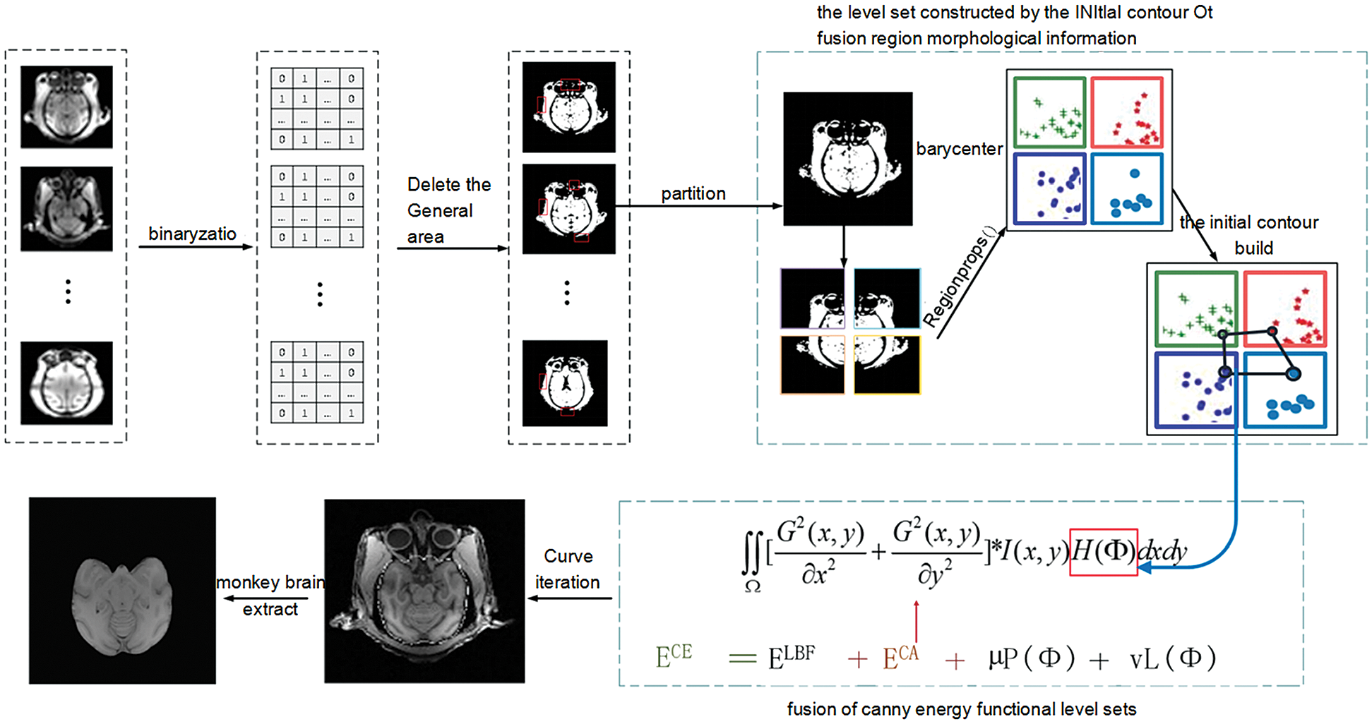
Figure 1: The overall architecture of our proposed method
As shown in Fig. 1, the model in this paper consists of two modules. The first module is an improvement of the initial contour construction algorithm. Based on the idea of partition, statistical analysis is performed on the morphological information of each region to establish the equation, and the initial contour is constructed to include the brain tissue of the macaque monkey to the maximum extent. The second module is to increase the processing of the edge information of brain tissue. Canny edge detection operator is fused in the LBF energy functional to achieve accurate detection of the edge of monkey brain tissue.
2.1 Initial Contour Construction Algorithm
Image binarization is the process of changing the gray value of pixel point to 0 or 255 according to the set threshold. The threshold th is assumed to exist, and all pixels of the image are divided into two categories, one is greater than the threshold th, and the other is less than the threshold th. The mean values of a1, a2 and the mean value of the whole image are calculated respectively. The optimal threshold for the best segmentation effect is calculated according to the following formula.
where, ω1 = number of background pixels/total pixels, ω2 = number of foreground pixels/total pixels.
2.1.2 Delete Small Connected Areas
The connected area of the image was counted, and the small non-brain tissue area was deleted by threshold setting. To compare the area of the small connected area of the rhesus monkey image and accurately select the threshold, Fig. 2 selected the statistical data of the 300, 310, 320 and 330 layers of the rhesus monkey brain of 32127 for display, and cut off the data with the area of the connected area greater than 1000. It can be found that the Area of small connected Area is concentrated around 200, so the threshold value of Area is preliminarily set as 200.
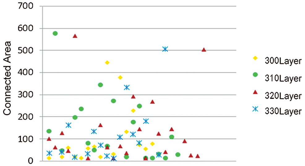
Figure 2: Scatter plots of connected areas in different layers of the same macaque
At the same time, the area of the connected area of the layers 230, 260, 280, 290, 310, 320, 330, 330, 340, 350, 360, 370, 380, 390 and 410 in no.32126 and no.32127 rhesus macaque MRI images were calculated. In Fig. 3, the statistical data with the connected area greater than 1000 are cut off, which better shows the statistical results of the data of small areas. It can be found from the box diagram that the box bodies of the connected area of the images of no.32126 and no.32127 macaques at different layers are mostly concentrated below 200. Therefore, in the step of deleting the small area connected area, the threshold is set as 200.
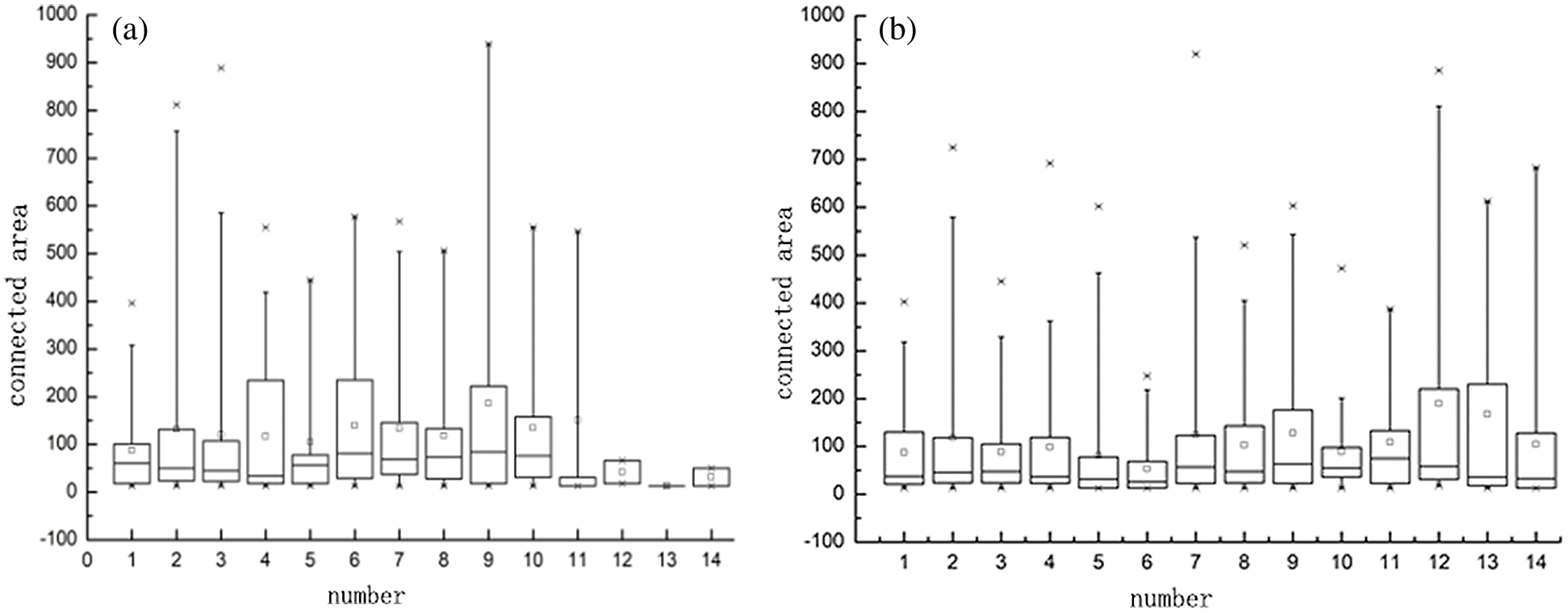
Figure 3: Box diagram of connected areas of different macaques. (a) 32126- Statistics of the small connected area of macaques and (b) 32127- Statistics of the small connected area of macaques
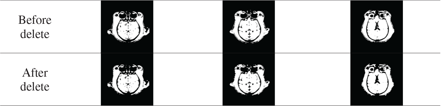
Tab. 1 shows the comparison results before and after deleting small connected regions. This step removes tissue such as the muscles around the eye and simplifies the calculation.
Table 1: Remove small area connectivity region results
To make the initial contour contain more target areas and improve the accuracy of monkey brain extraction, the image needs to be partitioned. Because the four local areas can maximize the coverage of the target area with the least amount of calculation, and the more target regions are included, the faster and more accurate the curve evolves. For any image A, divide it into four rectangular local areas as the seed areas for constructing the initial contour. The target image
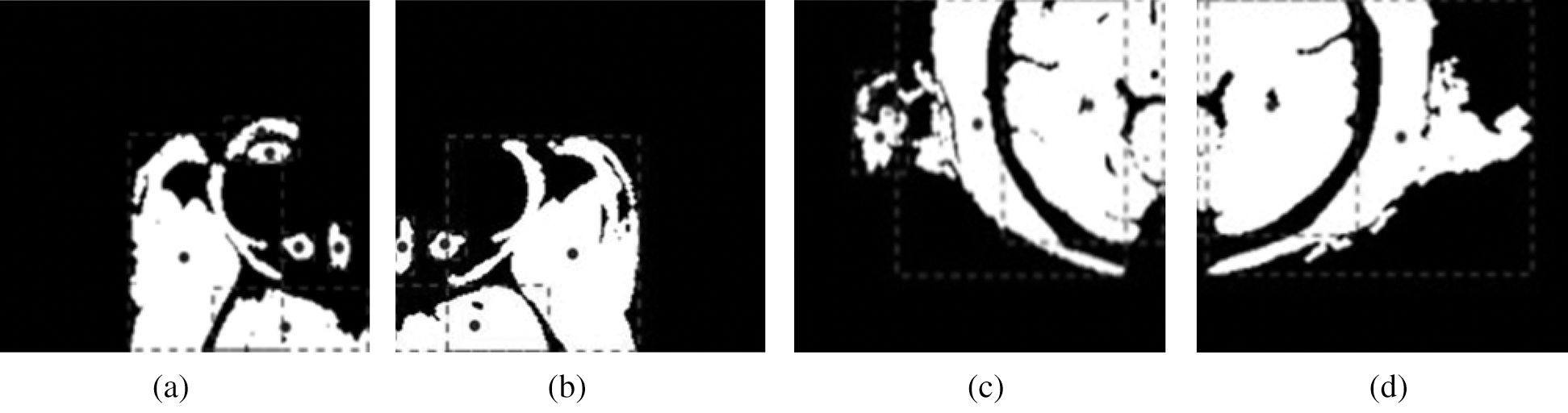
Figure 4: Centroid of each connected region in each rectangular region. (a) upper left, (b) upper right, (c) left lower and (d) right lower
The 300th layer image of rhesus monkey no. 32127 was divided into four local areas, and the centroid points of each connected region in each local area were calculated respectively. The results were shown in Fig. 4.
2.1.4 Initial Contour Construction
According to the morphological characteristics of the images, the monkey brain focusses on the image center and around the brain tissue adhesion. Therefore, the Euclidean distance between each centroid point and the partition point is calculated based on the centroid points of each connected region. In each local area, the centroid point with the smallest Euclidean distance is selected as the seed point to construct the initial contour, and the construction of the initial contour is completed [32,33]. Tab. 2 shows the construction results of the initial contours (red curve) of the monkey brain at different levels randomly selected from different macaques.
Table 2: Results of constructing the initial contour

2.2 Fusing Canny’s Energy Functional
To improve the efficiency of monkey brain edge detection, the edge detection operator was fused in the traditional level set LBF energy functional [34–36]. Tab. 3 compares the experimental results of various edge detection operators.
Table 3: Comparison of edge detection results

Tab. 3 compares the detection results of the first-order edge detection operator (first row) and the second-order edge detection operator (second row) on the same image, it can be found based on the second derivative test results of edge detection operator is better than the first derivative edge detection operator. The Canny operator adds a non-maximum value suppression operation and a dual-threshold filtering process to make the edge curve continuous and the lines thinner, making the detection result more accurate. Therefore, the Canny operator and the level set energy function are selected for fusion to better detect the boundary of monkey brain tissue.
The horizontal set function shall conform to the characteristics of the symbolic distance function, which is defined as follows:
Among,
Introduce the level set function into the energy functional, and define the following LBF energy function:
Among,
When canny detects the edge, the noise is first removed by the Gaussian filter. The generation equation of the Gaussian filter with the size of:
After the filtering operation is completed, the convolution operation is carried out, that is, all pixels in the image should be weighted and summed with their surrounding pixels. The gradient amplitude and direction of all pixels in the image are obtained according to the following formula.
where,
where,
Also, the length term constraint function
In the evolution process, in order to prevent the horizontal set function from losing the characteristic of sign distance function and causing instability in the evolution process, the distance penalty term function was added in the energy functional to shorten the reinitialization process of the level set, so that the evolution process could be carried out smoothly.
Therefore, the total energy functional of the model in this paper is:
where,
The standard gradient descent flow is used to minimize the energy functional so that the
The gradient descent flow equation obtained by keeping
where,
The process of solving the minimum value of the horizontal set energy functional is the process of solving the minimum value of the partial differential equation. This process meets the requirements of using the finite-difference method. The image space belongs to the equipartition grid, so the finite-difference method is generally used for calculation. It should be noted that in the case of fixed space step h, the time step
where
The evolution equation of the level set function
where,
3 Analysis of Experimental Results
1. UC Davis Dataset. The data set collected data from 19 rhesus monkeys using the Siemens Skyra3T scanner. The data included structures T1 and T2, as well as task-state fMRI and dMRI. In this experiment, NMR data with structures T1 were used. All the 19 monkeys were females, ranging in age from 18.5 to 22.5 years. The weight distribution was 7.28-14.95kg. Scanning sequence parameters: voxel resolution = 0.3 × 0.3 × 0.3 mm, TE = 6.93 ms, TR = 15 ms, TI = 1100 ms, Flip Angle = 8°.
2. Mountsinai-P Dataset. Data of 9 macaques were collected by the Philips 3T scanner. The data included structures T1, T2, and dMRI. In this experiment, NMR data with structures T1 were used. The data set included 8 males and 1 female, with an age distribution of 3.4-8 years and a weight distribution of 4.7-7.42kg. The scanning sequence parameters were as follows: voxel resolution = 0.5 × 0.5 × 0.5 mm, TE = 6.93 ms, TR = 15 ms, TI = 1100 ms, Flip Angle = 8°.
3. Princeton Dataset. The data set used Simens Prisma VE11C 3T scanner to collect data from two rhesus monkeys. The data included structures T1, T2, dMRI, and task-state fMRI. In this experiment, NMR data with structures T1 were used. All the two macaques in the data set were male, with an age distribution of 3 years and a weight distribution of 4.7-5.5kg. Scanning sequence parameters were as follows: voxel resolution = 0.5 × 0.5 × 0.5 mm, TE = 2.32 ms, TR = 2700 ms, TI = 850 ms, Flip Angle = 9°.
4. Uminn Dataset. The data set was used to collect the data of 2 rhesus monkeys with Simens 7T scanner. The data included structures T1, T2, dMRI, and task-state fMRI. In this experiment, NMR data with structures T1 were used. All the two macaques in the data set were female, and their age distribution was over 10 years old. The scanning sequence parameters were as follows: voxel resolution = 0.3 × 0.3 × 0.3 mm, TE = 3.65 ms, TR = 2500 ms, TI = 1100 ms, Flip Angle = 7°.
Tab. 4 below shows some data of the above four experimental data sets.
Table 4: Experimental data set
Experiment one: The ce-LevelSet of the model in this paper was applied to UC Davis, Mountsinai-P, Princeton and Uminn, respectively, to verify the feasibility of the model in this paper. The default parameters of the model in this paper are: time step
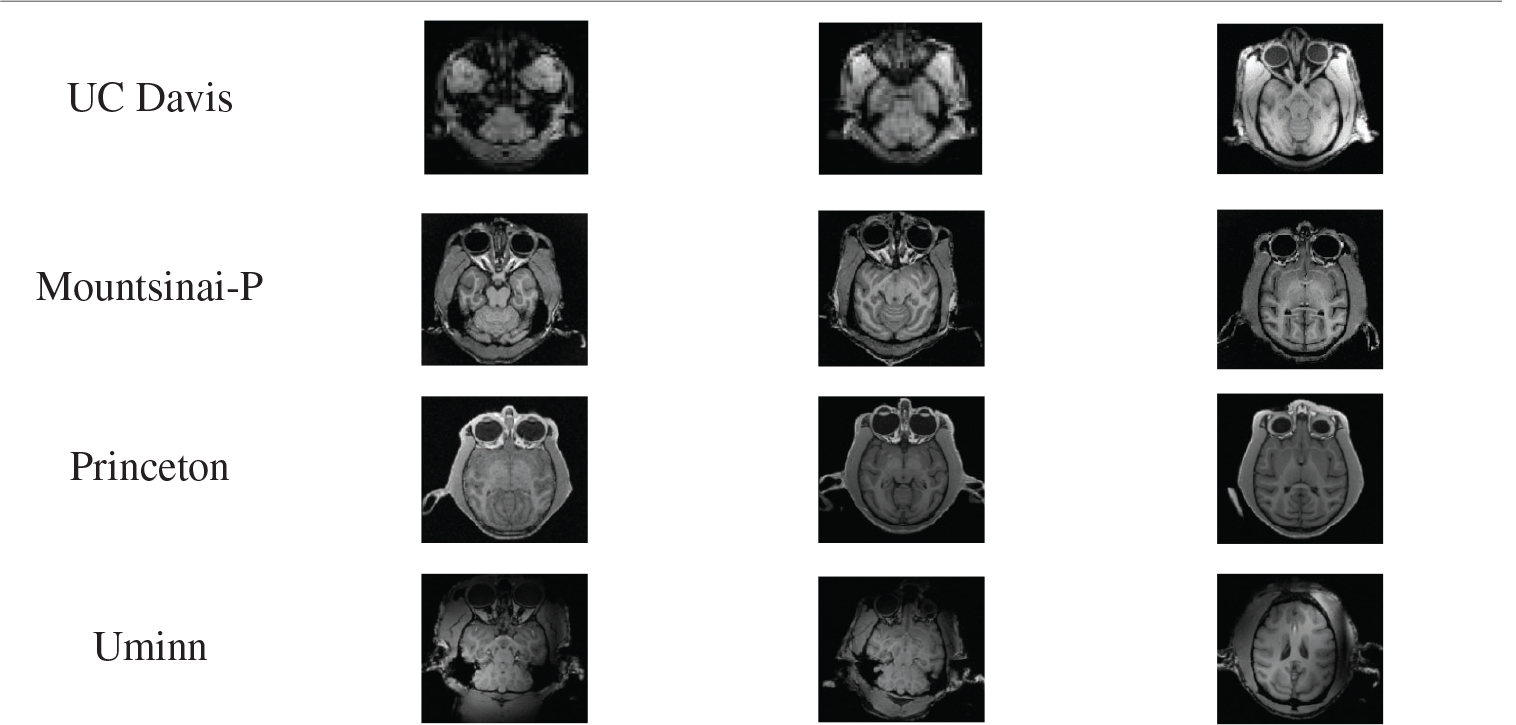
Tab. 5 shows the results of monkey brain tissue extraction after the model was applied to four sets of UC Davis, Mountsinai-P, Princeton and Uminn, and it can be found that the model applied to four different data sets in this paper can achieve complete extraction of monkey brain tissue, with good extraction effect.
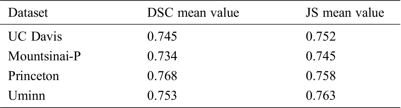
Tab. 6 shows the average value of DSC and JS of rhesus monkey brain tissue obtained after the model is applied to four data sets. From Tab. 6, it can be found that the monkey brain extraction results obtained after the model is applied to different data sets are good, and the similarity of DSC and JS with the standard brain tissue can reach about 0.75, and the performance is stable.
Table 5: Brain extraction results
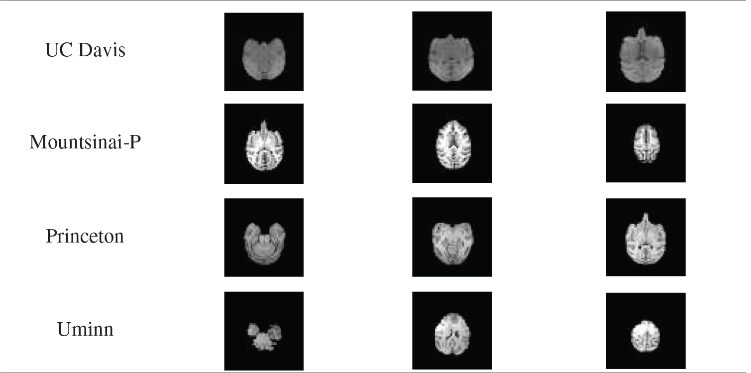
Table 6: The average value of DSC and JS values of the brain extracted by the model in different data sets
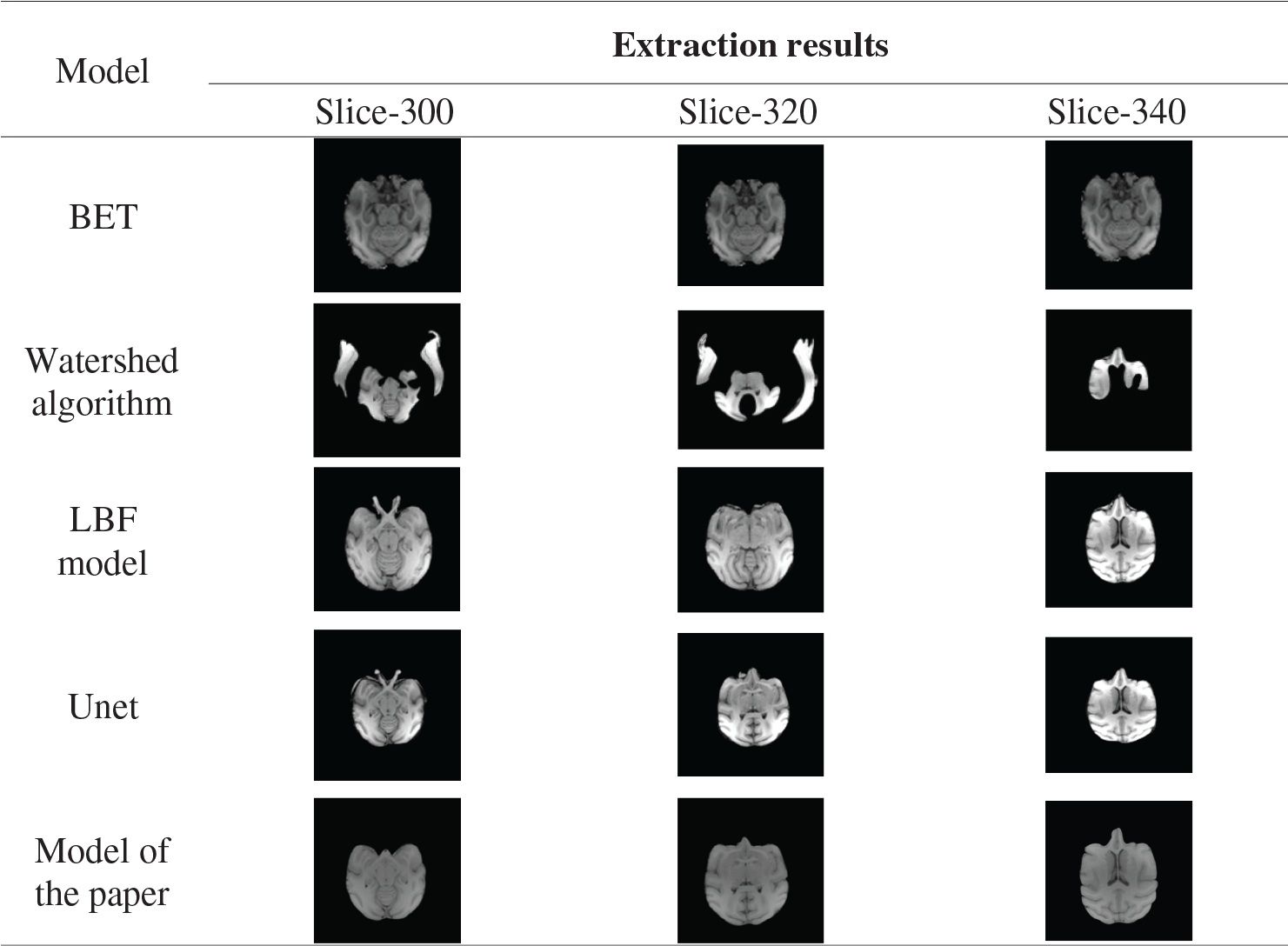
Experiment two: BET algorithm [37–39], watershed algorithm [40,41], LBF model and the model in this paper were used to extract the 300th, 320th, 340th and 360th layers of the brains of 32127 macaques in the UC Davis data set. A macaque brain image is cut into 512 layers according to the Z-axis [42], namely 512 images, each pixel size of 480
As can be seen from Tab. 7, the BET algorithm, LBF model, and Unet model cannot correctly peel off the fat and other non-brain tissues around the eyes, and their extraction effect on the edge part of brain tissues is poor. The Watershed algorithm cannot correctly extract brain tissue. In this paper, the model can accurately segment the eye and the temporal region and other muscle tissues, and the segmentation effect of the marginal region is better.
Table 7: Extraction results of different models
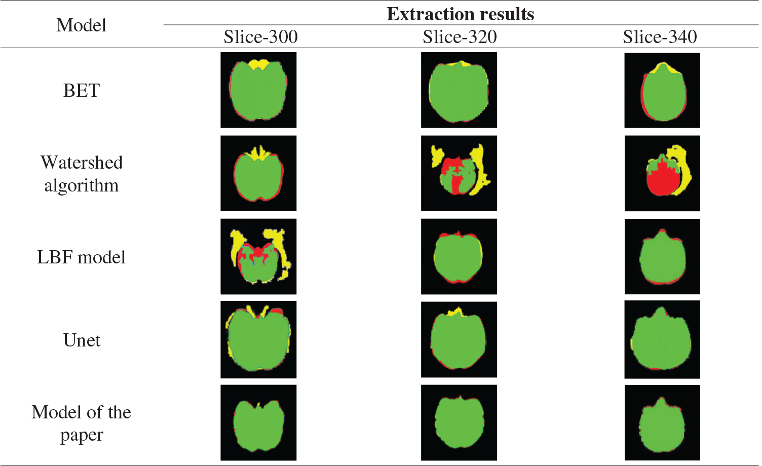
BET, watershed model, shown in Tab. 8 LBF model, Unet, this paper model the 300th floor of the monkey brain, 300, 320, 340 layers in the brain extract results as well as standard brain mask as a result, The red areas are the missing part of the mask extracted by the algorithm model compared with the standard mask, the yellow areas are the redundant part of the mask extracted by the algorithm model compared with the standard mask, and the green areas are the overlap between the mask extracted from the algorithm model and the standard mask. It can be seen from the table that the extraction results from BET, LBF, and Unet models include non-brain tissues such as muscles around the eyes, and the segmentation of marginal tissues such as the temporal region is inaccurate. The results of the watershed model include more non-brain tissue, such as skull, and more brain tissue regions, which are not accurately segmented. The results of the model extraction in this paper are accurate for the edge segmentation of brain tissue and clean for the separation of non-brain tissue.
Table 8: Extracted masks for different models
In order to more accurately compare the differences between the extraction results of different models, DSC and Jaccard similarity coefficient are used to carry out quantitative analysis on the experimental results. The DSC and Jaccard similarity coefficients range from 0 to 1 The closer the value is to 1, the higher the similarity is and the more accurate the segmentation result of the model is. On the contrary, the closer the similarity coefficient value is to 0, the lower the similarity is, and the worse the segmentation effect of the model is.
Table 9: Mean and standard deviation of DSC and JS values extracted by different models for the brain 32127
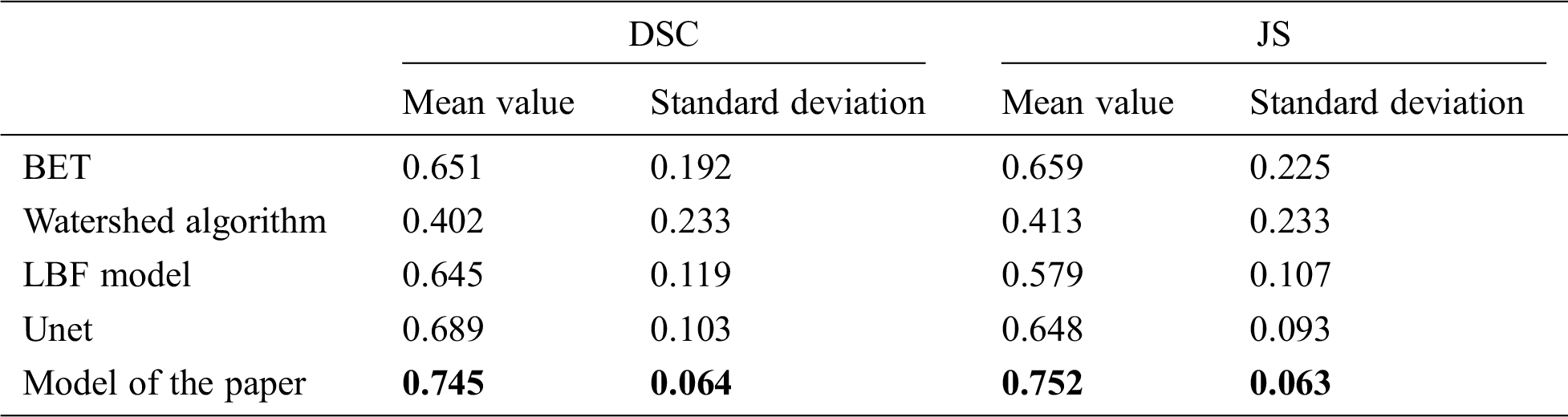
Tab. 9 shows the DSC and JS comparison results of the BET algorithm, watershed algorithm, LBF model, Unet, and the model in this paper after extracting the brain of 32127 rhesus monkeys. It can be found that the average value of DSC value and JS value of this model are 0.745 and 0.752, all take to its highest level in five models, the results show that this model of extracting similarity is higher than other models, at the same time, DSC and JS value standard deviation was 0.064 and 0.063, respectively, in the five models at the minimum, indicating that this model is more stable than other models, the results of the monkey brain images are extracted difference is smaller. The mean values of DSC and JS values of the other four models are all below 0.7, indicating that the monkey brain extraction results of these four models are poor. Meanwhile, the standard difference between DSC values and JS values can reach 0.1 or above, which is greater than the standard deviation of the model in this paper, indicating that these four models are less stable than the model in this paper.
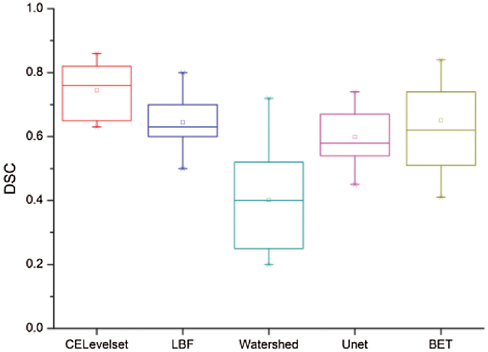
Figure 5: Dice similarity coefficient

Figure 6: Jaccard similarity coefficient
Fig. 5 shows that the median of the DSC value of the model in this paper is 0.78, which is the highest among the five models, the box body part between 0.82 0.67, The median of the DSC values of the LBF, Unet, and BET models are all in near 0.7, the LBF and Unet box parts are narrow, the BET model box part is between 0.5 0.75, the median of the DSC value of watershed algorithm is 0.42, and the box is between 0.23-0.48. we can get the brain tissue extract results of this model are the best.
Fig. 6 shows that the median of the JS value of the model in this paper is 0.78, which is the highest among the five models. the box body part between 0.81 and 0.66, LBF, the median of the DSC values of the LBF, Unet, and BET models are all in around 0.6, the LBF and Unet box parts are narrow, the box part of the BET model is between 0.52-0.77, we can get the brain tissue extract results of this model are the best.
Meanwhile, in this paper, the brain tissue of Monkey No. 32125 to 32136 was extracted using the above five models, and the DSC value and JS value of the extracted results were shown in Figs. 7 and 8.
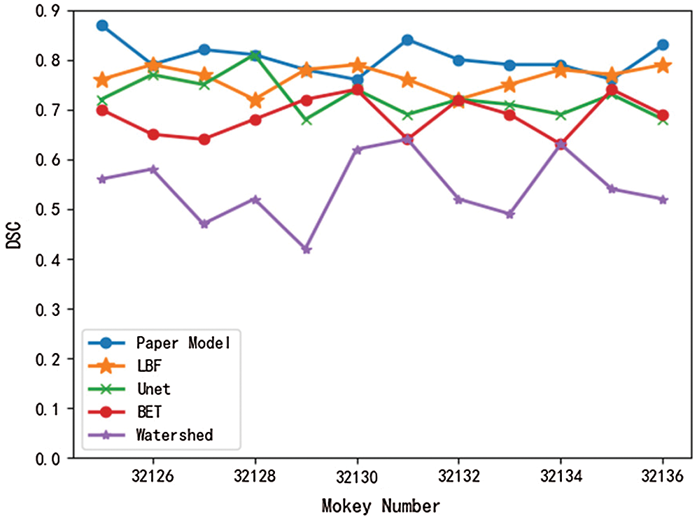
Figure 7: Comparison of DSC values of different models
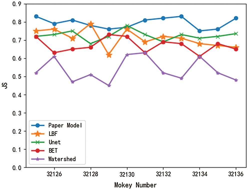
Figure 8: Comparison of JS values of different models
As can be seen from Figs. 7 and 8, DSC value and JS value in the brain tissue extraction results of different rhesus monkeys in the model presented in this paper perform well, at the highest value, and the model is relatively stable, with little difference in the extraction results for different rhesus monkeys. The extraction results of LBF, Unet, and BET models were significantly different and the models were unstable, while the extraction results of watershed models were poor and very unstable. In conclusion, compared with the other four models, DSC value and JS value in the experimental results of this model are close to 1, with a higher similarity coefficient and more accurate extraction results.
The automatic extraction of the macaque brain is the primary problem encountered in the research of the macaque brain. Therefore, this paper puts forward the RMCA-Level Set algorithm. First, the idea of partition is fused, and the initial contour is constructed by combining the mentality information of each region. The initial contour is constructed by binarization, deletion of small connected regions, and calculation of the center of mass by regions, etc., so as to improve the efficiency of brain tissue extraction. Secondly, to solve the problem of low edge extraction accuracy, a canny operator was fused into LBF energy functional to improve the extraction accuracy of the edge of brain tissue in this paper. Numerous experiments show that this model can be used to extract the brain tissue of the rhesus monkey.
Acknowledgement: Thank you for the National Natural Science Foundation of China, Natural Science Foundation of Shanxi Province, Key Research and Development Projects of Shanxi Province.
Funding Statement: This study was supported by research grants from the National Natural Science Foundation of China (61873178,61976150) and Key Research and Development Projects of Shanxi Province(201803D31038), Haifang Li received the grant and the URLs to sponsors’ websites is https://isisn.nsfc.gov.cn/egrantweb/ and http://kjt.shanxi.gov.cn/. This work was also supported by the Natural Science Foundation of Shanxi Province (201801D121135). Hongxia Deng received the grant and URLs to sponsors’ websites is http://kjt.shanxi.gov.cn/.
Conflicts of Interest: The authors declare that they have no conflicts of interest to report regarding the present study.
1. W. Yang, “The development of ultra-high field magnetic resonance imaging,” Physics, vol. 48, no. 4, pp. 227–236, 2019. [Google Scholar]
2. M. Quallo, C. J. Pric and K. UenoK, “Gray and white matter changes associated with tool-use learning in macaque monkeys,” in Proceedings of the National Academy of Sciences of the United States, New York, NY, USA, pp. 18379–18384, 2009. [Google Scholar]
3. K. M. Gilbert, J. S. Gati and K. Barker, “Optimized parallel transmit and receive radiofrequency coil for ultrahigh-field MRI of monkeys,” NeuroImage, vol. 125, pp. 153–161, 2016. [Google Scholar]
4. S. M. Smith, “Fast robust automated brain extraction,” Human Brain Mapping, vol. 17, no. 3, pp. 143–155, 2002. [Google Scholar]
5. T. Imtiaz, S. Rifat, S. A. Fattah and K. A. Wahid, “Automated brain tumor segmentation based on multi-planar superpixel level features extracted from 3D MR images,” IEEE Access, vol. 8, pp. 25335–25349, 2020. [Google Scholar]
6. Y. Ren, J. Qi, Y. Cheng, J. Wang and O. Asama, “Digital continuity guarantee approach of electronic record based on data quality theory,” Computers, Materials & Continua, vol. 63, no. 3, pp. 1471–1483, 2020. [Google Scholar]
7. L. Risser, L. Dolius and C. Fonta, “Diffeomorphic registration with self-adaptive spatial regularization for the segmentation of non-human primate brains,” in Proceedings of the Engineering in Medicine & Biology Society, Chicago IL USA, pp. 6695–6698, 2014. [Google Scholar]
8. M. A. El-Sayed, A. A. Alib and M. E. Hussien, “A multi-level threshold method for edge detection and segmentation based on entropy,” Computers, Materials & Continua, vol. 63, no. 1, pp. 1–16, 2020. [Google Scholar]
9. J. Doshi, G. Erus and Y. Ou, “Multi-atlas skull-stripping,” Academic Radiology, vol. 20, no. 12, pp. 1566–1576, 2013. [Google Scholar]
10. S. Dhifallah and I. Rekik, “Estimation of connectional brain templates using selective multi-view network normalization,” Medical Image Analysis, vol. 59, no. 1, pp. 1361–8415, 2020. [Google Scholar]
11. Y. Luo, B. Gao and Y. Deng, “Automated brain extraction and immersive exploration of its layers in virtual reality for the rhesus macaque MRI data sets,” Computer Animation and Virtual Worlds, vol. 30, no. 1, pp. 1841–1856, 2019. [Google Scholar]
12. Y. Ren, Y. Leng, J. Qi, K. S. Pradip, J. Wang et al., “Multiple cloud storage mechanism based on blockchain in smart homes,” Future Generation Computer Systems, vol. 115, no. 3, pp. 304–313, 2021. [Google Scholar]
13. J. Seidlitz, C. Sponheim and D. Glen, “A population MRI brain template and analysis tools for the macaque,” NeuroImage, vol. 170, no. 4, pp. 121–131, 2017. [Google Scholar]
14. J. Wang, W. Chen, L. Wang, Y. Ren and R. S. Sherratt, “Blockchain-based data storage mechanism for industrial Internet of Things,” Intelligent Automation & Soft Computing, vol. 26, no. 5, pp. 1157–1172, 2020. [Google Scholar]
15. G. Zhao, F. Liu and J. A. Oler, “Bayesian convolutional neural network based MRI brain extraction on nonhuman primates,” NeuroImage, vol. 175, pp. 32–44, 2018. [Google Scholar]
16. T. Li, Y. Ren and J. Xia, “Blockchain queuing model with non-preemptive limited-priority,” Intelligent Automation & Soft Computing, vol. 26, no. 5, pp. 1111–1122, 2020. [Google Scholar]
17. S. Qamar, H. Jin and R. Zheng, “A variant form of 3D-UNet for infant brain segmentation,” Future Generation Computer Systems, vol. 108, no. 5, pp. 613–623, 2020. [Google Scholar]
18. X. Y. Gong, S. Hu and X. De, “An overview of contour detection approaches,” International Journal of Automation and Computing, vol. 15, no. 6, pp. 656–672, 2018. [Google Scholar]
19. X. Chen, J. Chen and Z. Sha, “Edge detection based on generative adversarial networks,” Journal of New Media, vol. 2, no. 2, pp. 61–77, 2020. [Google Scholar]
20. X. Wang and Q. Pang, “Protoplasm somatic cells segmentation based on circle dependent fast level set segmentation,” Journal of Image and Graphics, vol. 18, no. 1, pp. 55–61, 2013. [Google Scholar]
21. G. Pan, L. Gao and S. Zhao, “Active contour model driven by local entropy energy,” Journal of Image and Graphics, vol. 18, no. 1, pp. 78–85, 2013. [Google Scholar]
22. F. M. Wang, H. Fan and Y. Wang, “Continuous level set algorithm based on improved CV model for magnetic resonance breast image segmentation,” Journal of Xi’an Jiaotong University, vol. 2014, no. 2, pp. 38–43, 2014. [Google Scholar]
23. C. Ge, Z. Liu, J. Xia and L. Fang, “Revocable identity-based broadcast proxy re-encryption for data sharing in clouds,” IEEE Transactions on Dependable and Secure Computing, vol. 16, no. 2, pp. 1–19, 2019. [Google Scholar]
24. Y. Ren, Y. Leng, Y. Cheng and J. Wang, “Secure data storage based on blockchain and coding in edge computing,” Mathematical Biosciences and Engineering, vol. 16, no. 4, pp. 1874–1892, 2019. [Google Scholar]
25. J. Wang, Y. Q. Yang, T. Wang, R. S. Sherratt and J. Y. Zhang, “Big data service architecture: A survey,” Journal of Internet Technology, vol. 21, no. 2, pp. 393–405, 2020. [Google Scholar]
26. D. Cao, B. Zheng, B. Ji, Z. Lei and C. Feng, “A robust distance-based relay selection for message dissemination in vehicular network,” Wireless Networks, vol. 26, no. 1, pp. 1755–1771, 2020. [Google Scholar]
27. K. Gu, X. Dong and W. Jia, “Malicious node detection scheme based on correlation of data and network topology in fog computing-based VANETs,” IEEE Transactions on Cloud Computing, vol. 8, no. 4, pp. 1–12, 2020. [Google Scholar]
28. X. F. Wang and D. S. Huang, “A novel density-based clustering framework by using level set method,” IEEE Transactions on Knowledge and Data Engineering, vol. 21, no. 11, pp. 1515–1531, 2009. [Google Scholar]
29. J. Wang, Y. Gao, W. Liu, A. K. Sangaiah and H. Kim, “An intelligent data gathering schema with data fusion supported for mobile sink in wireless sensor networks,” International Journal of Distributed Sensor Networks, vol. 15, no. 3, pp. 1–9, 2019. [Google Scholar]
30. R. Abdolvahab, M. R. Mohd, K. Hoshang and M. A. Ismail, “Morphological region-based initial contour algorithm for level set methods in image segmentation,” Multimedia Tools and Applications, vol. 76, no. 2, pp. 2185–2201, 2016. [Google Scholar]
31. J. Wang, X. Gu, W. Liu, A. K. Sangaiah and H. Kim, “An empower hamilton loop based data collection algorithm with mobile agent for WSNs,” Human-Centric Computing and Information Sciences, vol. 18, no. 9, pp. 1–14, 2019. [Google Scholar]
32. Y. Ren, F. Zhu, K. S. Pradip, J. Wang, T. Wang et al., “Data query mechanism based on hash computing power of blockchain in internet of things,” Sensors, vol. 20, no. 1, pp. 1–22, 2020. [Google Scholar]
33. A. E. Rad, M. S. M. Rahim and H. Kolivand, “Morphological region-based initial contour algorithm for level set methods in image segmentation,” Multimedia Tools and Applications, vol. 76, no. 2, pp. 2185–2201, 2016. [Google Scholar]
34. L. Xiang, W. Wu, X. Li and C. Yang, “A linguistic steganography based on word indexing compression and candidate selection,” Multimedia Tools and Applications, vol. 77, no. 5, pp. 28969–28989, 2018. [Google Scholar]
35. C. Ge, W. Susilo, Z. Liu, J. Xia, P. Szalachowski et al., “Secure keyword search and data sharing mechanism for cloud computing,” IEEE Transactions on Dependable and Secure Computing, vol. 17, no. 1, pp. 1–18, 2020. [Google Scholar]
36. A. Septiarini, H. Hamdani and H. R. Hatta, “Automatic image segmentation of oil palm fruits by applying the contour-based approach,” Scientia Horticulturae, vol. 261, no. 6, pp. 4238–4304, 2020. [Google Scholar]
37. R. Jin and G. Weng, “Active contours driven by adaptive functions and fuzzy c-means energy for fast image segmentation,” Signal Processing, vol. 163, no. 1, pp. 1–10, 2019. [Google Scholar]
38. W. Zhao, J. Liu, H. Guo and T. Hara, “ETC-IoT: Edge-node-assisted transmitting for the cloud-centric internet of things,” IEEE Network, vol. 32, no. 3, pp. 101–107, 2018. [Google Scholar]
39. J. Wang, Z. Sun and H. Ji, “A fast 3D brain extraction and visualization framework using active contour and modern openGL pipelines,” IEEE Access, vol. 7, pp. 156097–156109, 2019. [Google Scholar]
40. L. Song, C. Song and T. Zhuang, “Watershed-based brain magnetic resonance image automated segmentation,” Journal of Shanghai Jiaotong University, vol. 37, no. 11, pp. 1754–1756, 2003. [Google Scholar]
41. L. Fang, Y. Li, X. Yun, Z. Wen, S. Ji et al., “THP: A novel authentication scheme to prevent multiple attacks in SDN-based IoT network,” IEEE Internet of Things Journal, vol. 7, no. 7, pp. 5745–5759, 2020. [Google Scholar]
42. Y. Ren, Y. Liu, S. Ji, A. K. Sangaiah and J. Wang, “Incentive mechanism of data storage based on blockchain for wireless sensor networks,” Mobile Information Systems, vol. 2018, no. 8, pp. 1–10, 2018. [Google Scholar]
 | This work is licensed under a Creative Commons Attribution 4.0 International License, which permits unrestricted use, distribution, and reproduction in any medium, provided the original work is properly cited. |