DOI:10.32604/iasc.2021.017256
| Intelligent Automation & Soft Computing DOI:10.32604/iasc.2021.017256 | |
| Article |
Design and Experimentation of Causal Relationship Discovery among Features of Healthcare Datasets
Department of CSE, Pondicherry Engineering College, Puducherry, 605 014, India
*Corresponding Author: Y. Sreeraman. Email: sramany@gmail.com
Received: 25 January 2021; Accepted: 03 April 2021
Abstract: Causal relationships in a data play vital role in decision making. Identification of causal association in data is one of the important areas of research in data analytics. Simple correlations between data variables reveal the degree of linear relationship. Partial correlation explains the association between two variables within the control of other related variables. Partial association test explains the causality in data. In this paper a couple of causal relationship discovery strategies are proposed using the design of partial association tree that makes use of partial association test among variables. These decision trees are different from normal decision trees in terms of construction, scalability, interpretability and the ability of identifying causality in data. Normal Decision Trees are supervised machine learning approach to classify data based on a labeled attribute values. Variants of partial association trees are constructed as a part of analytics on a number of healthcare datasets. The applicability of design variants are carefully analyzed through this experimentation. In the above said experimentation it is found that the causation in data is not existed in data in some situations and sometimes the existing causality cannot be extracted where low associated dimensions are involved in data and hiding the underlying causality. One of the variants of proposed algorithms which was named dimensionality reduced partial association tree, did well in extracting causal association in case of a hidden causality in data.
Keywords: Supervised learning; causal relationship; data analytics; partial association tree
A normal decision tree is a supervised machine leaning approach that can be used to explore the relationship among data variables. It can test a data context for a target variant or class label. Causal relationships among data variables provide more useful knowledge for decision making. To find causal relationships experimentation is needed, but full experimentation is sometimes difficult to perform due to cost and ethical issues. When two variables are related it does not mean causation. A simple relation can be found using correlation, but not the causation.
Mantel et al. test [1] is a statistical test for repeated tests of independence when we have multiple 2 × 2 tables of independence. When there is an availability of observational data relating to a problem context, we can go for stratification of such data to convert it into multiple independent 2 × 2 tables. In this process a pair of variables acts as cause and effect variables and the rest is compounding variables. The chi-square value of the test is determined by the causal relationship between the pair of variables. Causal relationships can also be found from the data that was collected on observations [2]. Observational data needs hypothesis settings. If the automation is possible it must be competent with the ever increasing size of data. Though a decision tree is able to deal with observational data it is limited to the class prediction task [3]. A normal decision tree is not a suitable substitute for causal relationship mining. Therefore there is a need to construct a model that can identify the causality in data and can interpret the data context with respect to the underlying causalities.
In this paper a causal relation framework in the form of a decision tree which is based on partial association in data is constructed with a couple of assumptions about association, partial association, purity of the decision, and the strength of the decision at the concluding node. These assumptions lead to variants of design options for causal decision trees. This framework can identify the casual relationship between the predictor variable(s) and the outcome variable. The main contributions of this work include:
a) Design of a casual relationship discovery model
b) A systematic study of causal relationships among the data through various analytics.
c) Experimentation of the designed model on different healthcare datasets.
Causal analysis is an upcoming area in medicine and social sciences. Conclusion of causal relationship between two variables needs a lot of care when the decision is used for clinical applications [4]. Structural equation model is a deterministic model that interprets causality at population level [5]. A consequence of the causal inference research is a term recently came into existence that is “Decision Medicine” [6] which is nothing but treatment of patients based on causal inference from observational data. Probabilistic causality played a good role in past research [7]. After that Bayesian networks emerged as promising models for discovering causal structures [8–11]. He et al. [12] proposed models for finding prediction accuracy of the output results by combining Bayesian network based additive regression trees. They commented that the proposed model is better than existing algorithms in terms of speed and accuracy. Tree boosting algorithm is a well known and vital machine learning technique. Chen et al. [13] proposed advanced machine learning algorithm for sparse type data approximation with boosted tree based learning capability. This algorithm is faster in execution and wants lesser number of resources. In recent past constraint based approaches gained popularity in causal inference [14–16].
Though these model choices are quite interesting in idea, the applicability of these models has their own limitations. Some are demanding high experimentation cost. Some are facing the scalability problems. To deal with such situations observational study is a good alternative where the investigator does not intervene and rather simply “observes” and assesses the strength of the relationship between a predictor variable and a response variable. Recently some researchers proposed partial association rules to elevate casual relationships among data where the data is mostly observational [17,18].
Identifying cause of an outcome variable in data is a challenge task. Generally this task needs full experimentation which is not possible in many contexts due to the cost and other limitations of the experiment. Observational data play a vital role in cause identification, but analysis of observational data for cause identification needs a set of assumptions and computational overloads. The existing methods of causal discovery are suffering from scalability issues. The existing methods of causal relationship discovery have their own limitations in terms of experimentation cost, problem of high dimensionality, and scalability problems. Sometimes the nature of the data is also a significant limitation. To cope with such limitations better methodologies are in demand.
The proposed model is a decision tree where each splitting attribute is decided based on the strength of causal relationship between the current attribute and the goal attribute. To test the causality a statistical test named Mantel–Haenszel test for partial association [19] is used. This test is widely used to compare the outcome of two treatments based on stratification. The set of treatment variables of a dataset will be tested here to decide which variable has highest causal relationship. The attribute with highest partial association become the splitting attribute for the decision tree. At each node the process continues until the leaf nodes are generated based on some specified criteria.
Partial association test find the effect of a predictor variable on outcome variable in the presence of other compounding variables. Without these compounding variables the relation is just an association. The partial association in the context of other variables gives the partial association value and this value is used to determine the causality. This test is a tool to test the persistency of association between two variables given by other variables [20]. Partial association test eliminates inconsistencies that may risen by association rules.
Algorithm: Partial Association Tree (PAT)
Input
X = set of attributes (X1, X2… Xk-1, Y) where k is the dimension of the dataset.
D = dataset h = height of the tree
e = label of the edge (1 for left, 0 for right, −1 for initial edge and −1 for the root node)
Output: Partial association tree (PAT)
Steps:
1. Create root node T
2. Compute the correlation of Xi versus Y and trim the size of dimension by eliminating the attributes which are unable to meet the specified correlation threshold (follow this step for the algorithm variant named dimensionality reduced PAT)
3. Partial Association Tree Generation (T, X, D, D, h, e)
4. Prune Partial Association Tree: Prune (T)
Partial Association Tree Generation (T, X, D, D', h, e)
{
if (X is empty or (h + 1) = threshold or cardinality (D') < specified threshold (in the case of pre pruned PAT tree ) Then /*case-1 for leaf node creation with given threshold */
Create new treeNode and then find its class label as highest number among 0s or 1s of the outcome variable with respect to the current predictor variable (For extended PAT tree find the proportion values at the leaf nodes as the ratio of number of attributes with labeled decision value to total number of attributes at the current node. If the proportion value does not meet the sufficient threshold skip the following steps of leaf node creation)
if (e = 1) Then
add treeNode as left child of parent node, T
else
add treeNode as right child of parent node, T
end if
return
end if
find Correlation of Each Attribute in X (for partial association guided tree skip to the next step)
find PAT value for each correlation threshold satisfied attribute in X, where
Find one attribute whose PAT value is the largest. (for correlation guided tree find the PAT value of the attribute with largest correlation and consider it as largest PAT value)
if (largest PAT value <= 3.84) /* case-2 for creating leaf node */
Create new treeNode and then find its class label as highest number among 0s or 1s of the outcome variable with respect to the current predictor variable
if (e = 1) then
add treeNode as left child of parent node, T
else
add treeNode as right child of parent node, T
end if
return
end if
create new node W
if ( e = −1 ) Then
W = T //W will be the root node
else
add W as a child node of T
end if
X* = (X - best attribute with largest PAT value)
divide D into left data set, D1 and right data set, D2
call Partial Association Tree Generation (W, X*, D, D1, h, 1)
call Partial Association Tree Generation (W, X*, D, D2, h, 0)
Prune (T)
1. Repeat
2. for each leaf nodes in the Partial_Association_Tree do
2.1 if the present leaf node and its corresponding sibling leaf node have the same class label then convert their parent node into leaf node and label it with the appropriate class label.
2.2. delete both the leaf nodes
3. end for
4. until two sibling leaf nodes have different class labels
The proposed algorithm has a variable algorithm of six variants with respect to six cases.
Case-1: The given dataset is a collection of number of predictor attributes along with a decision attributes. The tree starts growing by determining a split attribute at each level of a tree. To identify a split attribute with current data in hand, first the correlation of each predictor attribute with the decision attribute will be computed. Based on the correlation threshold the PAT value of selected predictor variables to the decision variable is determined. A predictor attribute with the highest PAT value is the candidate for splitting attribute. The tree continues to grow until the following conditions are met:
a) the current node becomes a leaf node when the PAT value is not sufficient.
b) the current node becomes a leaf node when the tree reached a specified height or all the decision attributes have been exhausted. A pruning process is followed next to merge two leaves of a node with the same outcome label as a leaf at the parent node with the matched label. This process will continue for leaf pairs until no more pruning is possible.
Case-2: (Dimensionality reduction PAT tree): This case adds one pretest of correlation between each predictor variable versus the decision variable. The dimensionality of the dataset gets reduced based on the correlation values. With the reduced dataset the procedure mentioned in case-1 will be continued.
Case-3: (Correlation guided tree): This case select the top correlated attribute as the splitting attribute if it has the sufficient PAT value .The rest of the process is same as case-1.
Case-4: (Extended tree): This case search for the leaves where the proportion value (the ratio of the total tuples with current label value to the total number of attributes at the current node) is near to 50%, where stopping the tree growth is not a wise decision. Here instead of being a leaf node the current node grows further to provide more extension.
Case-5: (Pre pruned tree): This case stops the growth of the tree where the number of tuples at a node does not meet a specified threshold. The rest of the process is same as in case 1.
Case-6: (PAT value based tree without correlation): This case does not compute correlation values and does not require the same. The rest of the algorithm is same as in case 1.
10 datasets are considered for experimentation all of which are health and medical context. Majority of the datasets are sourced from UCI machine learning repository. To analyze the capability of the proposed approach various datasets with different sizes and dimensions are considered.
Dataset 1) Cardiovascular Disease dataset: It has twelve attributes. The value of target attribute decides whether the patient has heart problem or not. The size of this dataset is 70,000 which is sourced from Kaggle Progression System.
Dataset 2) Momographic mass (Bio chemical) dataset: It has six attributes. The value of outcome attribute decides about the severity of the bio chemical. The size of this dataset is 829.
Dataset 3) Vertebral Column Data Set: It has seven attributes. The value of class attribute decides whether the patient condition is normal or abnormal. The size of this dataset is 309.
Dataset 4) Health care dataset (stroke data): It has twelve attributes. The value of stroke attribute decides whether the patient got a stroke or not. The size of this dataset is 43400.
Dataset 5) Pima Indians Diabetes dataset: It has nine attributes. The value of outcome attribute decides whether to go for caesarian or not. The size of this dataset is 768.
Dataset 6) Breast Cancer dataset: This dataset have sixteen attributes. The value of diagnosis attribute decides whether the disease is benign or malignant. The size of this dataset is 568.
Dataset 7) Caesarian dataset: It has six attributes. The value of caesarian attribute decides whether to go for caesarian or not. The size of this dataset is 80.
Dataset 8) Indian liver dataset: It has eleven attributes. The value of Liver status attribute decides whether the patient has liver disease or not. The size of this dataset is 583.
Dataset 9) Insurance dataset: It has seven attributes. The value of charges attribute decides whether to pay < Rs.13271.0 or >= Rs. 13271.0 as insurance charge. The size of this dataset is 1338.
Dataset 10) Heart_Two dataset: It has seven attributes. The value of target attribute decides whether the patient has heart problem or not. The size of this dataset is 303.
6.1 Partial Association Tree Construction with Dataset1
Dataset1 (Cardio vascular disease dataset) with 70000 records is considered for experiment and explained the proposed algorithm variants. The results of the variants with findings are detailed below.
6.1.1 Partial Association Tree of Dataset1
From figure it is observed that the first variant of the algorithm produced a tree (Fig. 1) with four causal relation attributes { Resting ECG, Chest pain type, Exercise induced angina, and Fasting blood sugar}.Among these Resting ECG is the top level causal attribute with highest causality followed by the other attributes towards down the tree.

Figure 1: Partial Association Tree (PAT) E: Resting ECG, A: Chest pain type, G: Exercise induced angina, D: Fasting blood sugar
6.1.2 A Partial Association Tree with Dimension Reduced of Dataset1
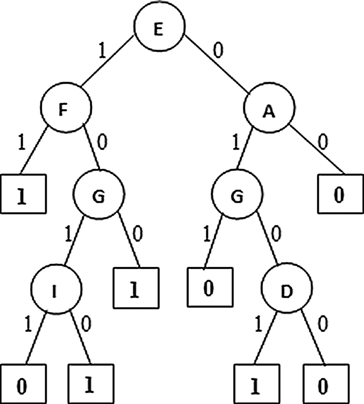
Figure 2: PAT with Dimensionality Reduction E: Resting ECG, F: Maximum heart rate achieved, A: Chest pain type, G: Exercise induced angina, D: Fasting blood sugar, I: Slope
From figure it is observed that the second variant of the algorithm named dimensionality reduction produced a tree (Fig. 2) with five causal relation attributes {Resting ECG, Maximum heart rate achieved, Chest pain type, Exercise induced angina, and Fasting blood sugar}. Among these Resting ECG is the top level causal attribute with highest causality followed by the other attributed towards down the tree. Here the dimensionality reduction variant produced more choices with one more attribute for decision making with respect to causality.
6.1.3 A Partial Association Tree Guided by Correlation of Dataset1

Figure 3: PAT through Correlation
This variant generated a Partial Association Tree (PAT) which is shown in Fig. 3 is same as the tree generated from the first variant. This similarity is signaling that for this particular dataset association among variables leading to causation also. For such data context this variant of the algorithm works well with lesser computations.
6.1.4 A Partial Association Tree with Extensions at Low Proportion Nodes of Dataset1
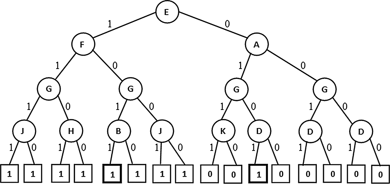
Figure 4: PAT without extension (non-pruned)
(Highlighted leaves with proportions near to 50% indicating traced labeling. Here proportion is the ratio of tuples with current label to total labels at the parent node)
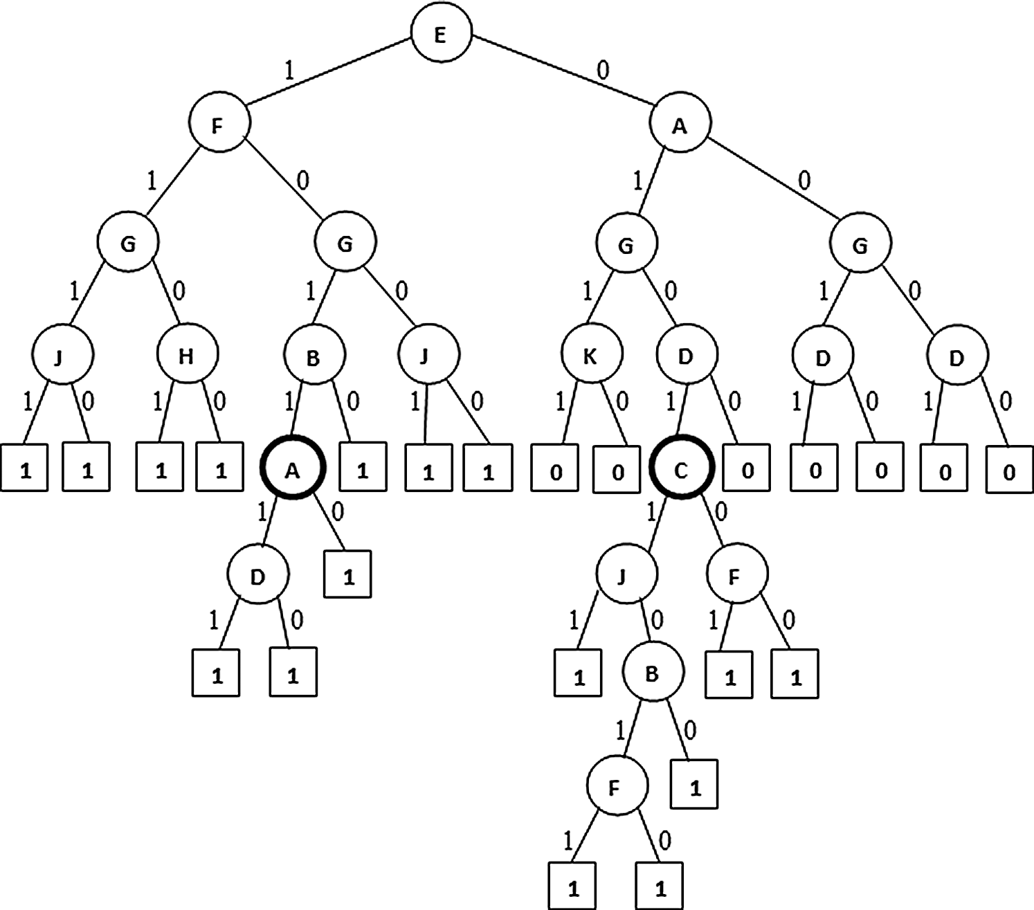
Figure 5: Extended PAT (non-pruned)
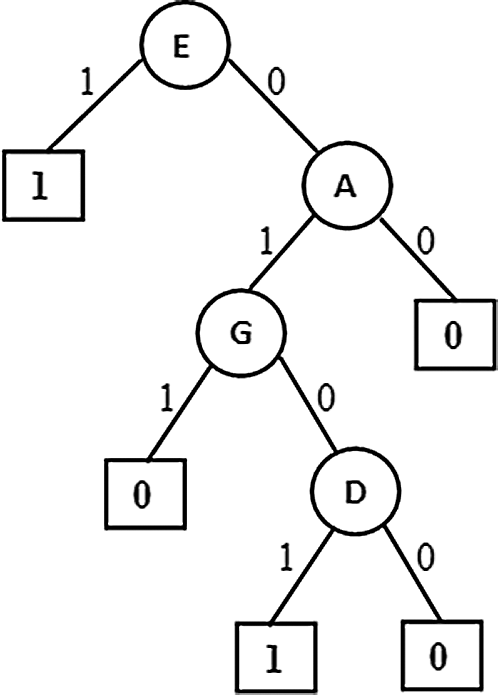
Figure 6: Pruned version of Extended PAT
In Figs. 4–6 the tree generation with the variant named extended PAT is presented. In Fig. 4 a partial association tree without extension is presented. Here at highlighted leaf nodes the proportion of the decision is very close to 50% which is really a trace situation where the chances of labels one and zero are almost equal and because of a little majority of chance one of the labels got selected. The present version of the algorithm tried to extend the tree to lower levels to get more precise information and the result is shown in Fig. 5. Here the tree grown up to further levels. This type of tree extension certainly put additional knowledge for decision making. The pruned version is shown in Fig. 6 which is again same as the one produced for the first variant.
6.1.5 A Partial Association Tree with Pre Pruning at Low Sized Nodes of Dataset1
The partial association tree with prior pruning done based on number of tuples participating at a node. If the participation is less than a minimum defined threshold then the current node become a leaf. Result of such algorithm variant is presented in Fig. 7. This variant is almost same as the first variant but differs slightly with the attribute set. This variant is promising when the observed data for some particular cases is too less and guides the user to invest such cases thoroughly.
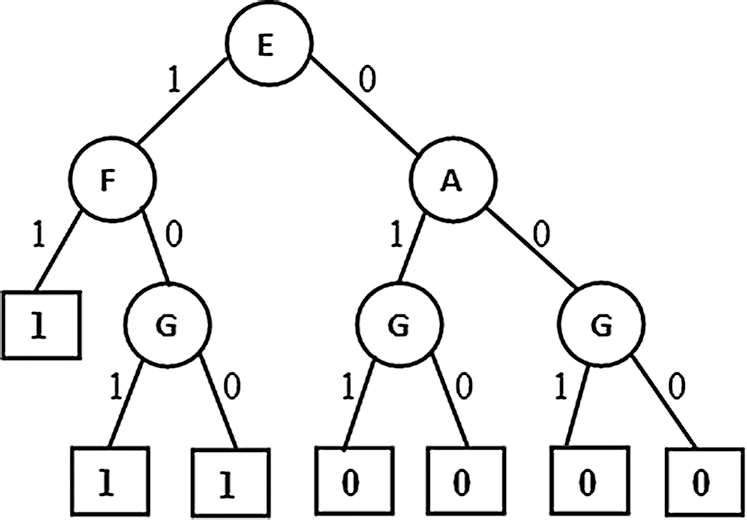
Figure 7: Pre Pruned PAT
6.1.6 A Partial Association Tree with No Correlation Computations of Dataset1
This variant generated a Partial Association Tree (PAT) shown in Fig. 8 is same as the tree generated from the first variant. When the dimensionality is low this variant is suitable with fewer computations where the saving is through non computation of correlation among the attributes. This similarity is signaling that for such data context with low dimensions this variant of the algorithm works well with lesser computations.

Figure 8: PAT without using correlation and based on PAT value only
6.2 Decision Tree Construction with Selected Datasets
Variants of the proposed algorithm are applied on the datasets dataset1 to dataset10. The comparative tables of results are given below.
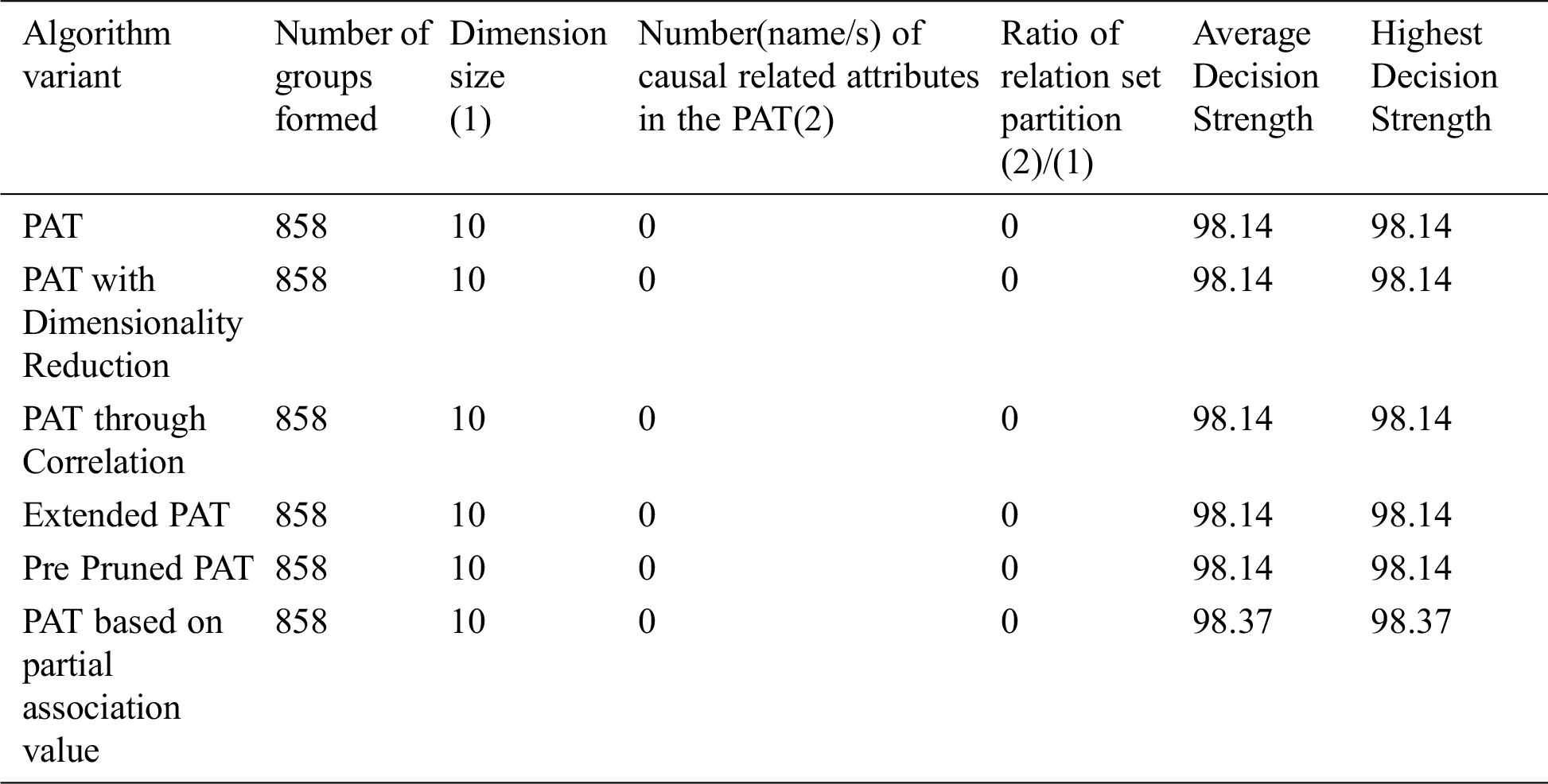
6.2.1 Variants of the Proposed Algorithm Are Applied on Dataset-1
The comparative table of results is given by Tab. 1. From Tab. 1 it can be observed that all variants of the algorithm provided almost the same decision tree which provides causality with the variables {restecg, chest_pain type, exang and fbs} of which restecg (resting electrocardiographic results) is the top level causal variable. When the dimensionality reduction is applied prior to the PAT tree generation there is no change in the resultant tree. So, in this context this variant of the algorithm only saved the computational effort.
Table 1: Comparative table for the dataset named “Cardiovascular Disease” & size-70000
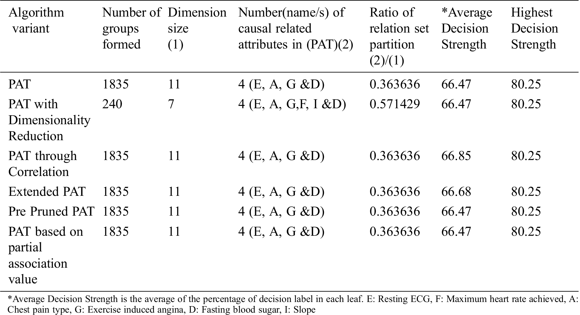
The comparative table of results is given by Tab. 1. From Tab. 1 it can be observed that all variants of the algorithm provided almost the same decision tree which provides causality with the variables {restecg, chest_pain type, exang and fbs} of which restecg (resting electrocardiographic results) is the top level causal variable. When the dimensionality reduction is applied prior to the PAT tree generation there is no change in the resultant tree. So, in this context this variant of the algorithm only saved the computational effort.
6.2.2 Variants of the Proposed Algorithm Are Applied on Dataset-2
Table 2: Comparative table for the dataset named “Momographic mass” & size-829
From Tab. 2 it can be observed that all variants of the algorithm provided almost the same decision tree with no attributes except the variant dimensionality reduction with which provides causality in the variable {margin} which itself is the top level causal variable. So, when the dimensionality reduction is applied prior to the PAT tree generation there is a change in the resultant tree with one guiding attribute and with the decision strength improved. So, in this context this variant of the algorithm provided a meaningful decision tree which is not possible with other variants and also providing more decision strength comparing to the other variants. It is also found that when the dimensionality is reduced, number of subgroups of data reduced significantly and it leads to extraction of hidden causality.
6.2.3 Variants of the Proposed Algorithm Are Applied on Dataset-3
Table 3: Comparative table for the dataset named “Vertebral column” & size-309
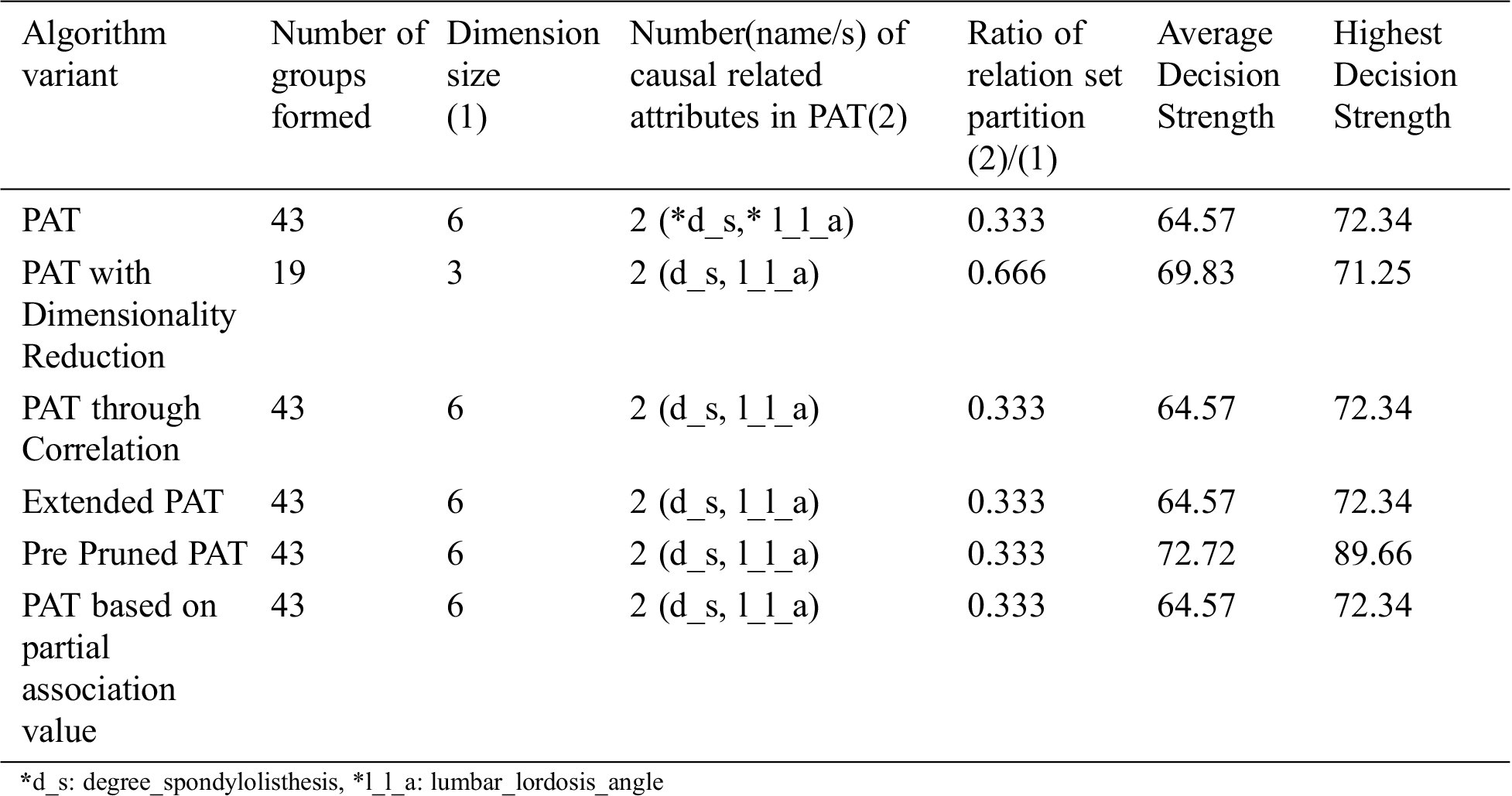
From the above Tab. 3 it can be observed that all variants of the algorithm provided almost the same decision tree which provides causality with the variables {degree_spondylolisthesis, lumbar_lordosis_angle} of which degree_spondylolisthesis is the top level causal variable. When the dimensionality reduction is applied prior to the PAT tree generation there is no change in the resultant tree. So, in this context the variant of the algorithm is saved by the computational effort.
6.2.4 Variants of the Proposed Algorithm Are Applied on Dataset-4
The comparative table of results is given by Tab. 4. From Tab. 4 it can be observed that all variants of the algorithm provided almost the same decision tree which causality is there but with no visual tree as a result of pruning. Pruning covered the casualty existed in data. This is an indication of almost the absence of causality in data. So in this context this variant of the algorithm only saved the computational effort.
Table 4: Comparative table for the dataset named “Health Care” & size-43400
6.2.5 Variants of the Proposed Algorithm Are Applied on Dataset-5
Table 5: Comparative table for the dataset named “Pima Indian” & size-768
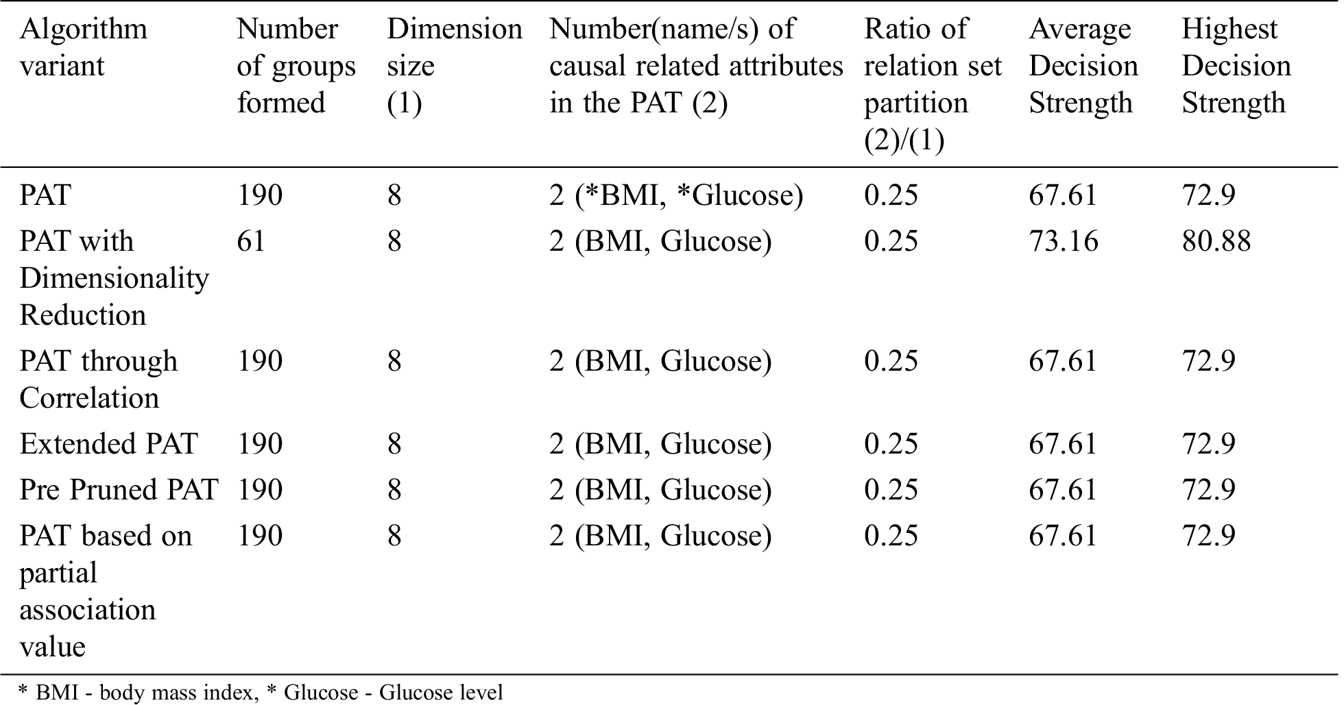
The comparative table of results is given by Tab. 5. From Tab. 5 it can be observed that all variants of the algorithm provided almost the same decision tree which provides causality with the variables of which BMI is the top level causal variable. When the dimensionality reduction is applied prior to the PAT tree generation there is no change in the resultant tree but the decision strength is improved. So, in this context this variant of the algorithm provided more decision strength comparing to the other variants.
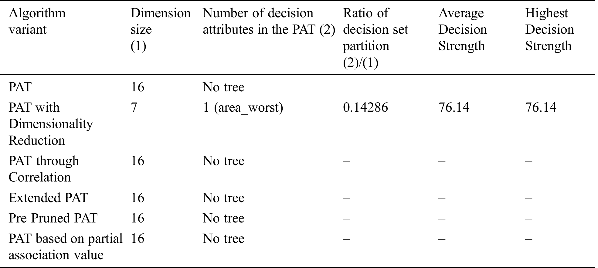
6.2.6 Variants of the Proposed Algorithm Are Applied on Dataset-6
From Tab. 6 we conclude that PAT with Dimensionality reduction only generated the tree and with remaining variants tree is not possible.
Table 6: Comparative table for the dataset named “Breast Cancer” & size-568
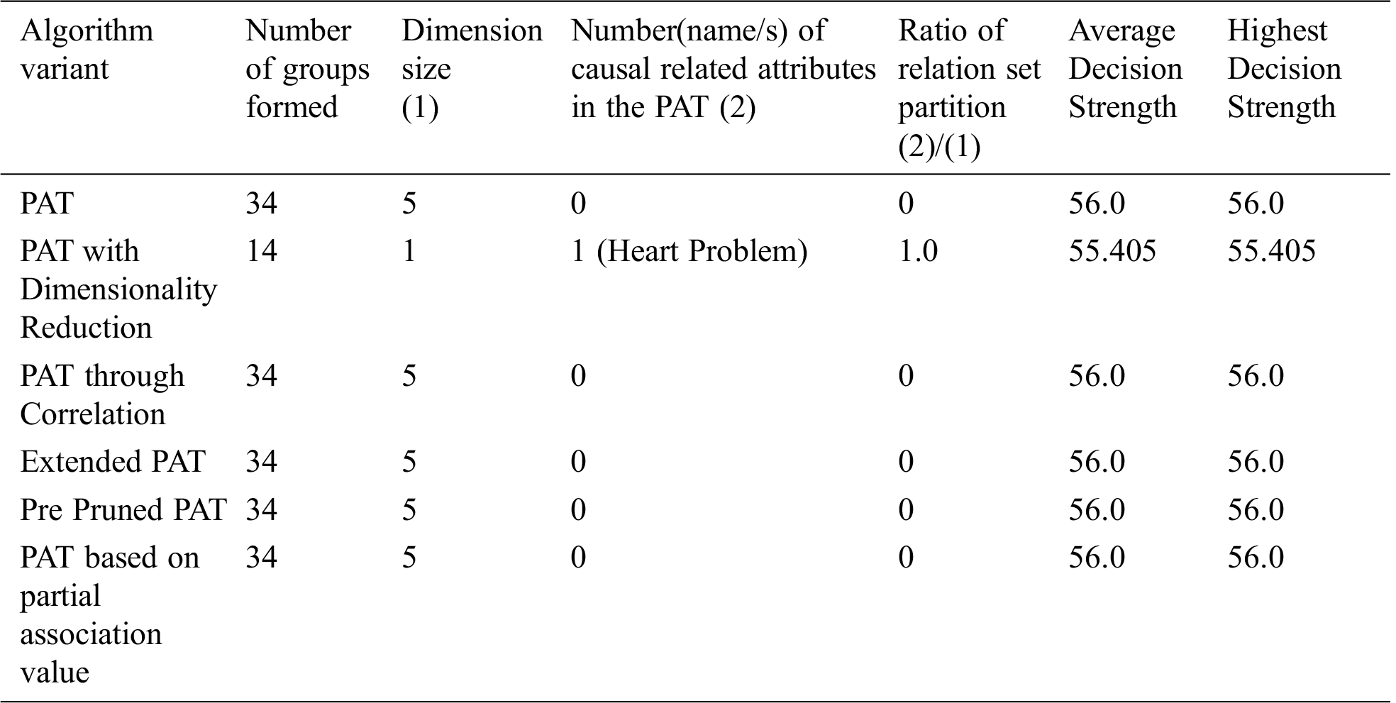
6.2.7 Variants of the Proposed Algorithm Are Applied on Dataset-7
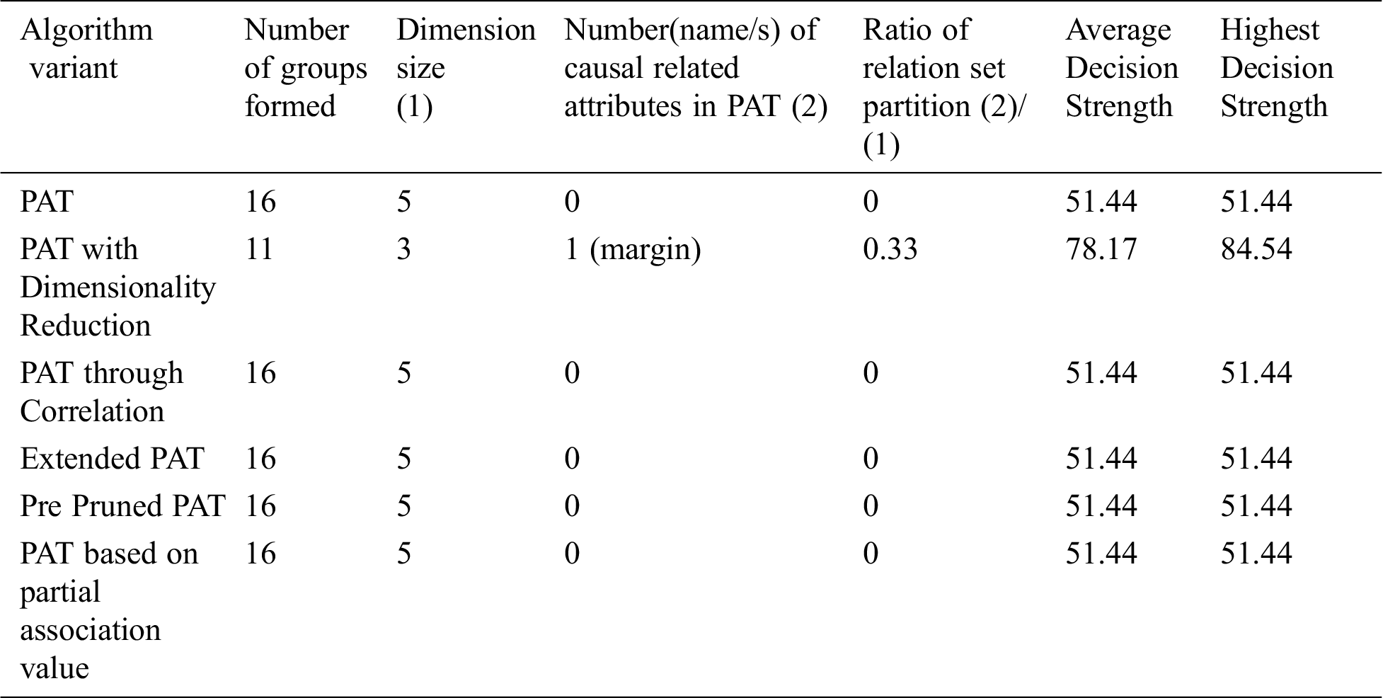
The result of partial association tree algorithm variants for the dataset named caesarian is presented in Tab. 7. All variants are produced by the decision trees with no decision attribute. It is a sign of no causality in data. The resultant tree before pruning showed some causality but the equal effect of all causal attributes made the decision tree null. From the table it can be observed that all variants of the algorithm provided almost the same decision tree with no attributes except the variant dimensionality reduction with which provides causality with the variable{heart problem} which itself is the top level causal variable. So, when the dimensionality reduction is applied prior to the PAT tree generation there is a change in the resultant tree with one guiding attribute. So, in this context the variant of the algorithm provided a meaningful decision tree which is not possible with other variants. It is also found that when the dimensionality is reduced, number of subgroups of data is reduced significantly and it leads to extraction of hidden causality.
Table 7: Comparative table for the dataset named “Caesarian” & size-80
6.2.8 Variants of the Proposed Algorithm Are Applied on Dataset-8
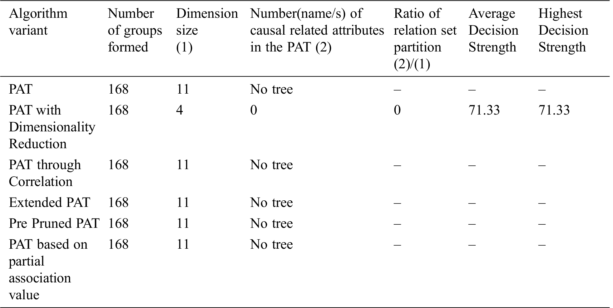
From Tab. 8 we conclude that PAT with Dimensionality reduction only generated the tree, later they are pruned and with remaining variants tree is not possible.
Table 8: Comparative table for the dataset named “Indian Liver” & size-583
6.2.9 Variants of the Proposed Algorithm Are Applied on Dataset-9
Table 9: Comparative table for the dataset named “Insurance” & size-1338
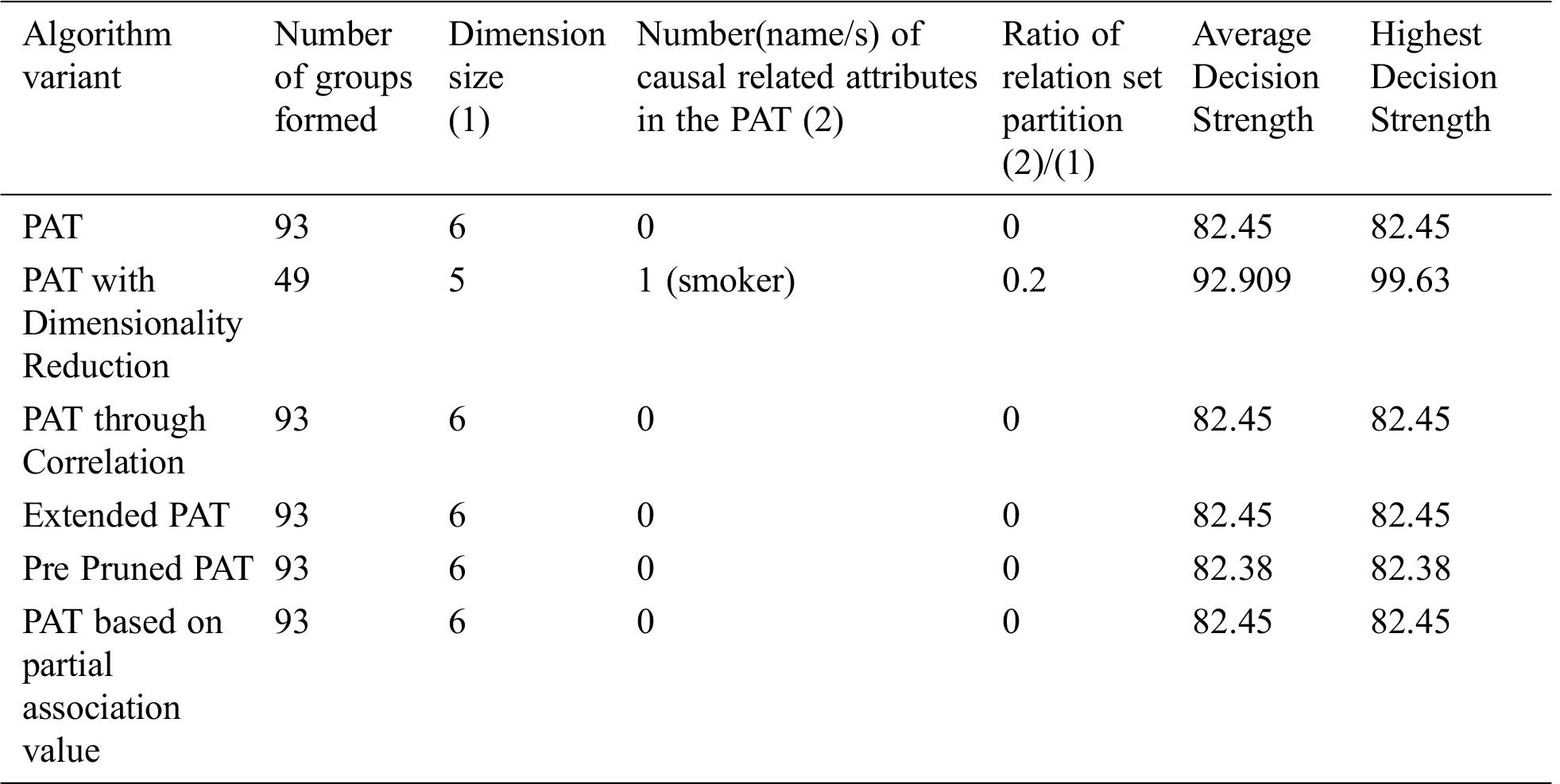
The comparative table of results is given by Tab. 9. The result of partial association tree algorithm variants for the dataset named caesarian is presented in Tab. 9. All variants produced by the decision trees with no decision attribute. It is a sign of no causality in data. The resultant tree before pruning showed some causality but the equal effect of all causal attributes made the decision tree null. From the above table it can be observed that all variants of the algorithm provided almost the same decision tree with no attributes except the variant dimensionality reduction with which provides causality with the variable{smoker} which itself is the top level causal variable. So, when the dimensionality reduction is applied prior to the PAT tree generation there is a change in the resultant tree with one guiding attribute. So, in this context this variant of the algorithm provided a meaningful decision tree which is not possible with other variants. It is also found that when the dimensionality is reduced, number of subgroups of data reduced significantly and it leads to extraction of hidden causality.
6.2.10 Variants of the Proposed Algorithm Are applied on Dataset-10
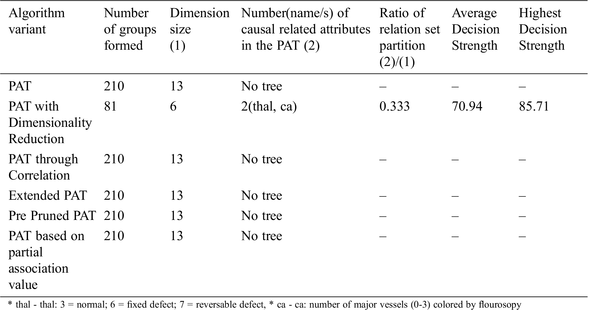
The comparative table of results is given by Tab. 10. The result of partial association tree algorithm variants for the dataset named Heart_Two is presented in Tab. 10. All variants produced the decision trees with no decision attribute. It is a sign of no causality in data. The resultant tree before pruning showed some causality but the equal effect of all causal attributes made the decision tree null. From the below table it can be observed that all variants of the algorithm provided almost the same decision tree with no attributes except the variant dimensionality reduction which provides causality with the variables{thal, ca} of which thal is the top level causal variable.
So, when the dimensionality reduction is applied prior to the PAT tree generation there is a change in the resultant tree with guiding attributes. So, in this context this variant of the algorithm provided a meaningful decision tree which is not possible with other variants. It is also found that when the dimensionality is reduced, number of subgroups of data reduced significantly and it leads to extraction of hidden causality.
Table 10: Comparative table for the dataset named “Heart_Two” & size-303
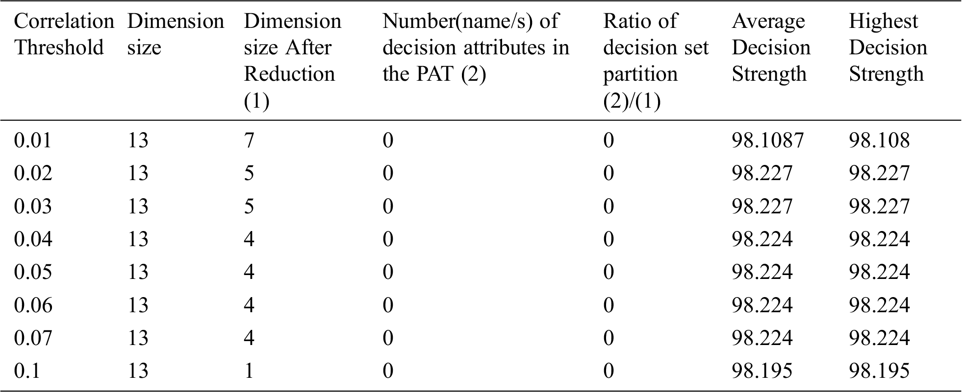
The result of the dimensionality reduction variant on dataset Heart_Two with varying dimensions by adjustment of correlation threshold is given in Tab. 11.
Table 11: Special Table for Heart_Two dataset using Dimensionality reduction
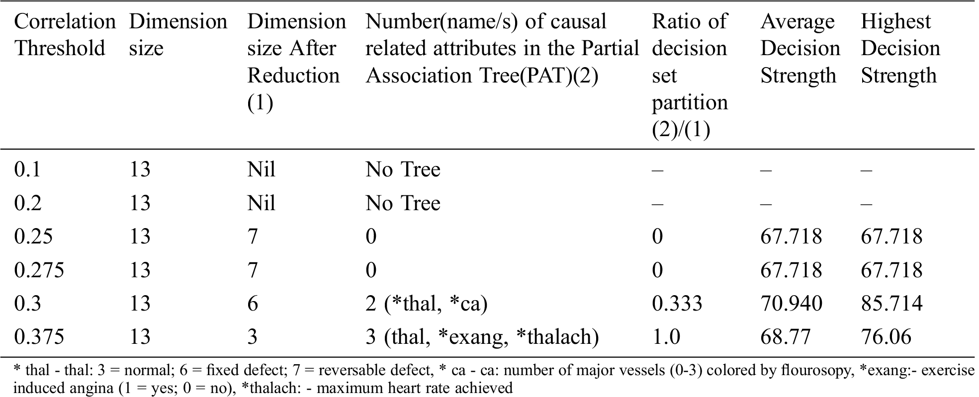
From the above table it is clear that dimensionality reduction (where poor correlation attributes are removed) works well and is able to generate decision tree (extract hidden causality). At the correlation threshold of 0.01 no dimension is reduced. At increased levels of correlations, dimensionality starts reducing and the tree is able to show causal relationships which are hidden at higher dimensions (due to the effect of poor correlated attributes).
The result of the dimensionality reduction variant on dataset Heart_One with varying dimensions by adjustment of correlation threshold is given in Tab. 12.
Table 12: Special Table for Heart One dataset using Dimensionality reduction
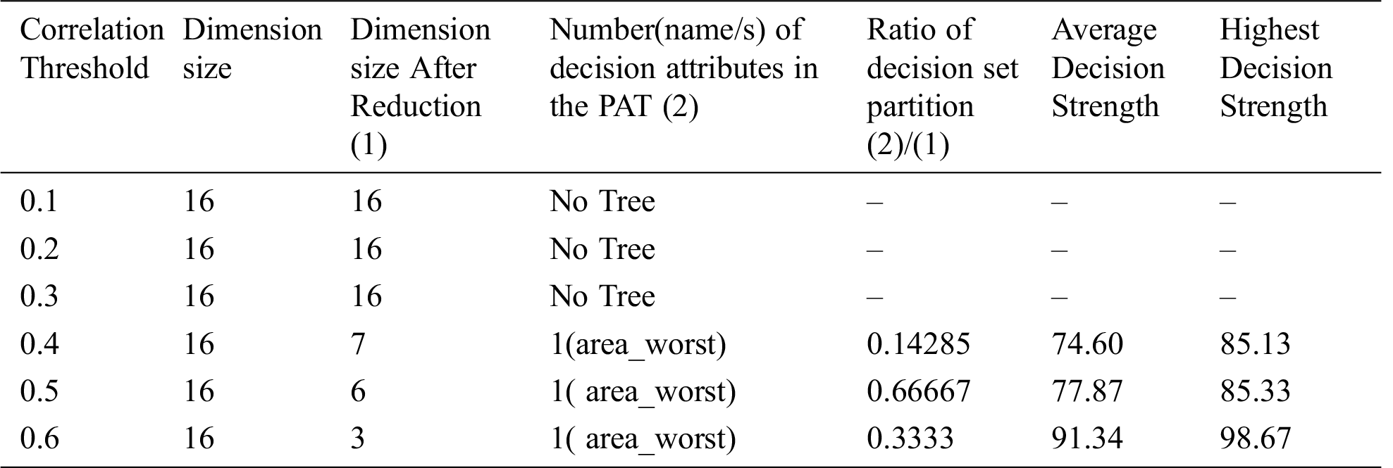
The result of the dimensionality reduction variant on dataset "breast cancer" with varying dimensions by adjustment of correlation threshold is given in Tab. 13.
From the three tables (Tabs. 11–13) it is clear that dimensionality reduction (where poor correlation attributes are removed) works well and is able to generate decision tree (extract hidden causality). At the correlation threshold of 0.01 no dimension is reduced. At increased levels of correlations, dimensionality starts reducing, and the tree is able to show causal relationships which are hidden at higher dimensions (due to the effect of poor correlated attributes). From Tab. 12, it can be observed that the dimensionality reduction is able to generate a tree but the same is hidden by the pruning process resulting zero nodes.
Table 13: Special Table for breast cancer dataset-6 using Dimensionality reduction
From the results obtained from six variant cases of the algorithm the following observations are made. The causal model which is developed in the form of partial association tree is able to give the casual relationships hidden in the data. The more the number of cases identified from the observational data the finer the knowledge that can be provided by the proposed model. To get maximum possible knowledge of causality from data it is needed to touch maximum possible data in terms of number tuples and number of cases of observations that are formed by the size of the dimension. Sometimes the real causation may be sheltered with excess attributes that are loosely associated with the decision variable. As a result the model cannot generate the tree. To uncover such causality a variant of the algorithm with dimensionality reduction is dependable. In some data contexts association among data can equally provide causality also. To observe such data contexts a variant of the algorithm where the tree construction is guided by correlations existed in data is promising. In some situations the strength of a causal relationship in terms of the number of tuples associated with the decision is fuzzy. To deal with such cases either pre pruning or extension versions of the algorithm are the alternatives to make the causal relation more clear.
Extracting causality from data is an intense area of research in data analytics. A causal inference model named Partial Association Tree is proposed in this paper. To meet with different sizes and contexts of data, some variants of the model are exercised to mine interpretable knowledge from data. All the model variants are applied on different datasets observed from medical and related contexts. The proposed algorithm is able to extract causality from data which is not possible from normal decision trees. The proposed model is more suitable than the existing models of causal inference. Using the variants of the proposed model a post optimal analysis is made. This analysis certainly shows the way to deal with datasets with underlined causality but hidden due to the nature, formation and dimensionality of data. The suitability of different variants of the proposed model is studied, and the possibilities are presented with sufficient experimentation. The gist of this approach can offer more research in the area of causal relationship mining.
Funding Statement: The authors received no specific funding for this study.
Conflicts of Interest: The authors declare that they have no conflicts of interest to report regarding the present study.
1. N. Mantel and W. Haenszel, “Statistical aspects of the analysis of data from retrospective studies of disease,” National Cancer Institute, vol. 22, no. 4, pp. 719–748, 1959. [Google Scholar]
2. P. R. Rosenbaum, “Design of observational studies,” in The Springer Series, 1st ed., vol. 1. Berlin, Germany: Springer, 65–94,2010. [Google Scholar]
3. P. N. Tan, M. Steinbach and V. Kumar, “Introduction to data mining,” in The Pearson. Upper Saddle River, NJ, USA: Pearson, pp. 37–69, 2006. [Google Scholar]
4. K. J. Rothman, S. Greenland and T. L. Lash, “Modern epidemiology,” in The Library of Congress Catalog, 3rd ed., Lippincott Williams and Wilkins, pp. 5–31,2008. [Google Scholar]
5. J. Pearl, “The Causal foundations of Structural equation modeling,” in The Handbook of Structural Equation Modeling, R. H. Hoyle ed.,New York: Guilford Press, pp. 68–91,2011. [Google Scholar]
6. K. A. Goddard, W. A. Knaus, E. Whitlock, G. H. Lyman and H. S. Feigelson, “Building the evidence base for decision making in cancer genomic medicine using comparative effectiveness research,” Genetics in Medicine, vol. 14, no. 7, pp. 633–642, 2012. [Google Scholar]
7. J. Pearl, “Probabilistic reasoning in intelligent systems: Networks of plausible inference,” In: The Morgan Kaufmann Series in Representation and Reasoning, Revised 2nded., San Mateo, CA: Morgan Kaufmann, pp. 14–23,1988. [Google Scholar]
8. J. Pearl, “From bayesian network to causal networks,” in The Mathematical Models for Handling Partial Knowledge in Artificial Intelligence. Plenum Press, pp. 157–182,1995. [Google Scholar]
9. D. Heckerman, “A Bayesian approach to learning causal networks,” in Proc. UAI’95, San Francisco, CA, USA, pp. 285–295, 1995. [Google Scholar]
10. N. L. Zhang and D. Poole, “Exploiting causal independence in Bayesian network inference,” Artificial Intelligence Research, vol. 5, no. 1, pp. 301–328, 1996. [Google Scholar]
11. S. Nadkarni and P. P. Shenoy, “A Bayesian network approach to making inferences in causal maps,” Operational Research, vol. 128, no. 3, pp. 479–498, 2001. [Google Scholar]
12. J. He, S. Yalov and P. Richard Hahn, “Accelerated bayesian additive regression trees,” in Proc. AISTAS, Naha, Okinawa, Japan, vol. 89, pp. 1130–1138, 2019. [Google Scholar]
13. T. Chen and C. Guestrin, “XGBoost: A scalable tree boosting system,” in Proc. ACM SIGKDD, San Francisco, CA, USA, pp. 785–794, 2016. [Google Scholar]
14. S. Mani, P. L. Spirtes and G. F. Cooper, “A theoretical study of Y structures for causal discovery,” in Proc. UAI, San Francisco, CA, USA, pp. 314–323, 2006. [Google Scholar]
15. J. P. Pellet and A. Elisseeff, “Using markov blankets for causal structure learning,” Machine Learning Research, vol. 9, pp. 1295–1342, 2008. [Google Scholar]
16. C. F. Aliferis, A. Statnikov, I. Tsamardinos, S. Mani and X. D. Koutsoukos, “Local causal and markov blanket induction for causal discovery and feature selection for classification part i: Algorithm and empirical evaluation,” Machine Learning Research, vol. 11, pp. 171–234, 2010. [Google Scholar]
17. J. Li, T. D. Le, L. Liu, J. Liu, Z. Jin et al., “Mining causal association rule,” in Proc ICDMW. Dallas, Texas, USA, pp. 114–123, 2013. [Google Scholar]
18. Y. Sreeraman and S. Lakshmana Pandian, “Data analytics and mining in healthcare with emphasis on causal relationship mining,” Recent Technology and Engineering, vol. 8, no. 4, pp. 195–204, 2019. [Google Scholar]
19. J. Zhang and D. D. Boos, “Generalized cochran-mantel-haenszel test statistics for correlated categorical data,” Communications in Statistics - Theory and Methods, vol. 26, no. 8, pp. 1813–1837, 1997. [Google Scholar]
20. J. Li., L. Liu and T. Le, “Causal rule discovery with partial association test in: Practical approaches to causal relationship exploration,” in The Springer Briefs in Electrical and Computer Engineering. Springer, pp. 33–50, 2015. [Google Scholar]
 | This work is licensed under a Creative Commons Attribution 4.0 International License, which permits unrestricted use, distribution, and reproduction in any medium, provided the original work is properly cited. |