Intelligent Automation & Soft Computing DOI:10.32604/iasc.2021.017586
Article

Parameter Estimation of Alpha Power Inverted Topp-Leone Distribution with Applications

Gamal M. Ibrahim1, Amal S. Hassan2, Ehab M. Almetwally3,*and Hisham M. Almongy4

1High Institute for Management Sciences, Belqas, 35511, Egypt
2Faculty of Graduate Studies for Statistical Research, Cairo University, Giza, 12613, Egypt
3Faculty of Business Administration, Delta University for Science and Technology, Mansoura, 11152, Egypt
4Faculty of Commerce, Mansoura University, Mansoura, 35516, Egypt
*Corresponding Author: Ehab M. Almetwally. Email: ehabxp_2009@hotmail.com
Received: 03 February 2021; Accepted: 21 March 2021

Abstract: We introduce a new two-parameter lifetime model, referred to alpha power transformed inverted Topp-Leone, derived by combining the alpha power transformation-G family with the inverted Topp-Leone distribution. Structural properties of the proposed distribution are implemented like; quantile function, residual and reversed residual life, Rényi entropy measure, moments and incomplete moments. The maximum likelihood, weighted least squares, maximum product of spacing, and Bayesian methods of estimation are considered. A simulation study is worked out to evaluate the restricted sample properties of the proposed distribution. Numerical results showed that the Bayesian estimates give more accurate results than the corresponding other estimates in the majority of the situations. The flexibility of the suggested model is demonstrated given some applications related to reliability, medicine, and engineering. A real data set is used to illustrate the potentiality of the alpha power transformed inverted Topp-Leone distribution compared to inverted Topp-Leone, inverse Weibull, alpha power inverse Weibull, inverse Lomax, alpha power inverse Lomax, inverse exponential, and alpha power exponential distributions. Criteria measures and their results showed that the suggested distribution is the best candidate for the considered data sets. The alpha power transformed inverted Topp-Leone distribution operates well for lifetime modeling.

Keywords: Inverted Topp-Leone; moments; maximum likelihood; maximum product spacing; weighted least squares; Bayesian estimation; MCMC

1  Introduction

In recent times, probability distributions play a significant role in modeling naturally occurring phenomena. In fact, the statistics literature contains hundreds of continuous univariate distributions and their successful applications. However, there still remain many real-world phenomena involving data, which do not follow any of the traditional probability distributions. So, several attempts are introduced by many researchers to provide more flexibility to a family of distributions. Mahdavi et al. [1] introduced the alpha power transformation (AP) technique by adding an extra shape parameter to well- known baseline distributions. The cumulative distribution function (CDF) of the AP method is defined by:

FAP(x)=[αG(x)−1α−1, α>0,α≠1G(x),    α>0,α=1. (1)

Relevant works have been provided based on the AP method, for instance; AP Weibull distribution [2], AP generalized exponential distribution [3], AP extended exponential distribution [4], AP Lindley distribution [5], AP power Lindley distribution [6], AP inverse Lindley distribution [7], AP exponentiated Lomax distribution [8] and AP inverse Lomax distribution [9].

The inverted distributions were suggested in the literature using the inverse transformation of probability distributions. These distributions display different features in the behavior of the density and hazard rate shapes. They allow applicability to the phenomenon in many fields such as; biological sciences, life testing problems, survey sampling, and engineering sciences. Inverted distributions and their applications were discussed by several authors (see [10–18]).

In Hassan et al. [18], the CDF and the probability density function (PDF) of the inverted Topp-Leone (ITL) distribution with shape parameter λ is defined as follows:

G(x; λ)=1−{(1+2x)λ(1+x)2λ};x≥0, λ>0, (2)

and,

g(x;λ)=2λx(1+x)−2λ−1(1+2x)λ−1;x,λ>0. (3)

In this paper, we propose a new two-parameter related to the ITL distribution depending on the AP family. We call it alpha power inverted Topp Leone (APITL) distribution. The basic motivations to introduce the APITL model are (i) Generalizing a new useful version of the ITL distribution based on the APT method along with deriving its statistical properties, (ii) Providing flexible PDF with right-skewed and uni-modal shapes, (iii) Modeling decreasing, increasing, upside-down hazard rate function (HRF), and (iv) Introducing some real applications in some areas.

This paper is constructed as follows. Section 2 describes the APITL distribution. Section 3 gives some structural properties of the APITL distribution. Section 4 gives the maximum likelihood (ML), the weighted least squares (WLS), the maximum product of spacing (MPS), and Bayesian estimators. Section 5 examines the effectiveness of the proposed estimates through a numerical illustration. Data analyses and some concluding remarks are employed, consequently, in Sections 6 and 7.

2  Description of the Model

In this section, based on the AP family we introduce a new probability distribution related to the ITL distribution. We define the PDF, CDF, HRF and cumulative HRF of the APITL distribution.

Definition 2.1

A random variable X is said to have the APITL distribution when we substitute the CDF (Eq. (2)) and PDF (Eq. (3)) in CDF (Eq. (1)). The CDF of a random variable X has the APITL distribution with parameters α and λ denoted by X ~ APITL (α,λ), is defined by:

F(x;α,λ)=[ α1−{(1+2x)λ(1+x)2λ}−1(α−1),x,α,λ>0,α≠1, 1−{(1+2x)λ(1+x)2λ},x,α,λ>0,α=1 . (4)

The PDF related to Eq. (4) is given by:

f(x;α,λ)=[ \matrix2λlog(α)x(1+x)−2λ−1(1+2x)λ−1α1−{(1+2x)λ(1+x)2λ}(α−1),x,λ,α > 0,α≠1  2λx(1+x)−2λ−1(1+2x)λ−1,  x,λ,α > 0,α=1 . (5)

Descriptive PDF plots of the APITL distribution for some choices of parameters are represented in Fig. 1. It can be seen that the PDF of APITL distribution is uni-modal as well as possesses a long tail right-skewed.

Figure 1: The PDF plots of the APITL distribution

Definition 2.2

The reliability function and the HRF of X are given by:

F¯(x;α,λ)=[ α−α1−{(1+2x)λ(1+x)2λ}α−1, x,λ,α>0,α≠1 (1+2x)λ(1+x)−2λ,x,λ,α>0,α=1 ​​, (6)

and

h(x;α,λ)=[ 2λlog(α)x(1+x)−2λ−1(1+2x)λ−1α1−{(1+2x)λ(1+x)2λ}α−α1−{(1+2x)λ(1+x)2λ},x,λ,α>0,α≠1 2λx[(1+x)(1+2x)]−1,       x,λ,α>0,α=1 . (7)

An illustration of the HRF plots for the APITL distribution, for some choices of α and λ, is represented in Fig. 2. It describes the HRF plots of the APITL distribution which can be decreasing, increasing, and upside down shaped.

Figure 2: The HRF of the APITL distribution

3  Distributional Properties

Here, we give some statistical properties.

3.1 Quantile Function

The APITL distribution is simulated by inverting CDF Eq. (4) as follows:

x=Q(x)=F−1(u),0<u<1. (8)

The uth quantile for the APITL random variable is obtained by solving F(x) = u for x as follows:

xu=−2[(1−K)1λ−1]+4[(1−K)1λ−1]2−4((1−K)1λ)(((1−K)1λ−1)2(1−K)1λ, (9)

where, K=(log⁡u(α−1)+1)(log⁡α)−1. The 25th, 50th, and 75th percentiles for the random variable X is obtained by setting u = 0.25, 0.5 and 0.75 in Eq. (9). The Bowley’s skewness, depends on quartiles, is defined as follows:

SKB=Q(3/4)−2Q(1/2)+Q(1 /4)Q(3 /4)−Q(1/2), (10)

where Q(.) is the APITL quantile function. The Moor’s kurtosis is given as:

KUm=Q(7/8)−Q(5/8)−Q(3/8)+Q(1/8)Q(6/8)−Q(2/8), (11)

Skewness and kurtosis plots of the APITL model, based on the quantiles, are exhibited in Fig. 3.

Figure 3: 3D Plots of (a) Skewness and (b) Kurtosis of the APITL distribution

3.2 Moments

Moments of a probability distribution are crucial to deduce its properties such as measures of central tendency, dispersion, skewness, and kurtosis. The ordinary rth moment of the APITL distribution is derived. The rth moment of the APITL distribution is obtained from Eq. (5) as follows:

μr′=2λlog⁡(α)(α−1)∫0∞xr+1(1+x)−2λ−1(1+2x)λ−1α1−{(1+2x)λ(1+x)2λ}dx. (12)

Since the power series representation is written as:

αx=∑i=0∞(log⁡α)ii!xi. (13)

Using the power series expansion Eq. (13) in Eq. (12), then we get

μr′=2λ(α−1)∑i=0∞(log⁡α)i+1i!∫0∞xr+1(1+x)−2λ−1(1+2x)λ−1[1−{(1+2x)λ(1+x)2λ}]idx. (14)

Using the binomial expansion in Eq. (14) then μr′ takes the form

μr′=2λ(α−1)∑i=0∞∑j=0i(−1)j(ij)(log⁡α)i+1i!∫0∞xr+1(1+x)−2λ(j+1)−1(1+2x)λ(j+1)−1dx. (15)

After using binomial expansion, then the rth moment is given by:

μ′r=2λ(α−1)∑i,m=0∞∑j=0i(−1)j(ij)(λ(j+1)−1m)(log⁡α)i+1i!∫0∞xr+m+1(1+x)−λ(j+1)−m−2dx.=∑i,m=0∞ξi,j,mB(r+m+2,λ(j+1)−r),λ(j+1)>r,r=1,2,.... (16)

where, ξi,j,m=2λ(α−1)∑j=0i(−1)j(ij)(λ(j+1)−1m)(log⁡α)i+1i!.

The first four moments, for r = 1, 2, 3 and 4, of the APITL distribution are obtained from Eq. (16). The rth central moment (μr) of X is given by:

μr=E(X−μ1′)r=∑i=0r(−1)i(ri)(μ1′)iμr−i′. (17)

Values of mean (μ1′), variance (σ2), skewness (γ1), and kurtosis (γ2) of the APITL distribution for certain values of parameters are given in Tab. 1.

Table 1: Some moments values of the APITL distribution for specific values of parameters

We concluded from Tab. 1 that, as the value of λ increases and for fixed value of α, then values of μ1′, σ2, γ1, and γ2 are decreasing. As the value of α increases and for fixed value of λ , then values of μ1′, and σ2 are increasing, while the values of γ1 and γ2 decrease. The distribution is positively skewed and leptokurtic.

3.3 The Probability Weighted Moments

The class of probability-weighted moments (PWMs), denoted by Υs,q, s and q are positive integers, of a random variable X is defined as follows:

Υs,q=E[XsF(x)q]=∫−∞∞xsf(x)(F(x))qdx. (18)

Substituting Eq. (4), and Eq. (5) in Eq. (18), further using expansion Eq. (13) and binomial expansion in Eq. (18), then the PWM of the APITL distribution is obtained as follows:

Υs,q=∑i,d=0∞νm,k,i,dB(s+d+2,λ(m+1)−s). (19)

where, νm,k,i,d=∑m=0i∑k=0q(λ(m+1)−1d)(im)(qk)(−1)q−k+m2λ(log⁡(α))i+1(q+1)i(α−1)q+1i!.

3.4 Residual and Reversed Residual Life

The mth moment of the residual life (RLe), say Πm(t)=E[(X−t)m|X>t],m=1,2,.. uniquely determines F(x). The mth moment of the residual life of X is defined by:

Πm(t)=(F¯(t))−1∫t∞(x−t)mdF(x). (20)

Therefore, the mth moment of RLe for APITL distribution is obtained by substituting PDF Eq. (5) in Eq. (20), then employing binomial expansions and Eq. (13) as follows:

Πm(t)=(F¯(t))−1∑k,ℓ=0∞Ψk,i,ℓ,d(t)m−iB(i+ℓ+2,λ(d+1)−i,(1+t)−1), (21)

where Ψi,k,ℓ,d=∑i=0m∑d=0k(−1)m−i+d2λ(log⁡α)k+1k!(α−1)(mi)(kd)(λ(d+1)−1ℓ), and B(.,.,(1+t)−1) is the incomplete beta function. For m = 1, in Eq. (21) we obtain the mean RLe of the APITL distribution. Also, mth moment of the reversed RLe (RRLe) for the APITL distribution is given by:

ϵm(t)=(F(t))−1∑k,ℓ=0∞Ψi,k,ℓ,d(t)m−iB(i+ℓ+2,λ(d+1)−i,t/t(1+t)), (22)

where, Ψi,k,ℓ,d=∑i=0m∑d=0k(−1)m−i+d2λ(log⁡α)k+1k!(α−1)(mi)(kd)(λ(d+1)−1ℓ).

The mean of RRLe serves as the waiting time elapsed since the failure of an item on the condition that this failure had occurred.

3.5 Rényi Entropy

The entropy of a random variable measures the amounts of information (or uncertainty) contained in a random observation; i.e., large value of entropy indicates higher uncertainty in the data. Rényi entropy of X, for Υ>0 and Υ≠1, is defined by:

Re(x)=(1−Υ)−1log⁡(∫0∞(f(x))Υdx). (23)

Substituting PDF Eq. (5) in Eq. (23), we obtain Rényi entropy of the APTIL model as follows:

Re(x)=(1−Υ)−1log⁡[(2λlog⁡(α)(α−1)Υ)Υ∫0∞xΥ(1+x)−Υ(2λ+1)(1+2x)Υ(λ−1)αΥ[1−{(1+2x)λ(1+x)2λ}]dx]. (24)

From Eq. (24), and after simplification, the Rényi entropy of the APITL distribution will be:

Re(x)=(1−Υ)−1log⁡{∑j,k=0∞Φj,m,kB(Υ+k+1,λΥ+λm+Υ−1)}, (25)

where, Φj,m,k=∑m=0j(Υlogα)j(−1)mj!(2λlog⁡(α)(α−1)Υ)Υ(jm)(Υ(λ−1)+λmk).

4  Parameter Estimation of the APITL Model

In this section, we deal with parameter estimators of the APITL distribution based on ML, WLS, MPS, and Bayesian estimation methods.

4.1 ML Estimators

Let X1,…, Xn e the observed values from the APITL distribution with parameters α and λ. The likelihood function, say L(x_|α,λ) of the APITL distribution is expressed as:

L(x_|α,λ)=2nλn(log⁡(α))n(α−1)−nαn−∑i=1n(1+2xi)λ(1+xi)2λ∏i=1nxi(1+2xi)λ−1(1+xi)2λ+1. (26)

Then the log-likelihood function, say ℓ, of the APITL distribution is given as:

ℓ=nlog⁡(2λ)+nlog⁡(log⁡(α))−nlog⁡(α−1)+nlog⁡(α)−log⁡(α)∑i=1n(1+2xi)λ(1+xi)2λ+∑i=1nlog⁡(xi)+(λ−1)∑i=1nlog⁡(1+2xi)−(2λ+1)∑i=1nlog⁡(1+xi). (27)

Therefore, the ML equations are given by:

∂ℓ∂α=1α[n+nlog(α)−∑i=1n(1+2xi)λ(1+xi)2λ]−nα−1, (28)

and,

∂ℓ∂λ=nλ−log(α)∑i=1n(1+2xi)λ(1+xi)2λlog((1+2xi)(1+xi)2)+∑i=1nlog(1+2xi)−2∑i=1nlog(1+xi). (29)

Solving the non-linear equations (∂ℓ/∂α)=0 and (∂ℓ/∂λ)=0 numerically using optimization algorism as conjugate-gradient optimization, we get the ML estimators of α and λ.

4.2 WLS Estimators

Let X1,…, Xn be a simple random sample from the APITL distribution and let X(1)< X(2)<…<X(n) be the associated order statistics. The WLS estimators of α and λ are attained by minimizing the following:

W(x_|α,λ)=∑i=1n(n+1)2(n+2)i(n−i+1)(Ξ(x(i))−in+1)2, (30)

Ξ(x(i))=(α−1)−1(α1−{(1+2x(i))λ(1+x(i))2λ}−1). Furthermore, the WLS estimators followed by solving the following nonlinear equations:

2∑i=1n(n+1)2(n+2)i(n−i+1)(Ξ(x(i))−in+1)Λs(x(i));s=α,λ. (31)

where Λα(x(i))=α−{(1+2x(i))λ(1+x(i))2λ}[(1+2x(i))λ(1+x(i))2λ(1−α)−1]+1(α−1)2 and Λλ(x(i))=α1−{(1+2x(i))λ(1+x(i))2λ}(α−1)((1+2x(i))(1+x(i))2)λln⁡(α)ln⁡((1+2x(i))(1+x(i))2).

4.3 MPS Estimators

The MPS method is an alternative procedure of the ML method which provides a parameter estimate of continuous distribution. The MPS estimators of α and λ are attained by maximizing the following:

ℓ(g)=1n+1{ln⁡(Ξ(x(1)))+∑i=2nln(Ξ(x(i))−Ξ(x(i−1)))+ln⁡(1−Ξ(x(n)))}. (32)

Solving the non-linear equations (∂ℓ(g)/∂α)=0 and (∂ℓ(g)/∂α)=0 via numerical technique, we obtain the MPS estimators of α and λ. To obtain the MPS estimators, we differentiate natural logarithm of the product spacing function of APITL distribution partially for α and λ.

∂ℓ(g)∂α=1n+1[Λα(x(1))Ξ(x(1))+∑i=2n(Λα(x (i))−Λα(x (i−1)))Ξ(x(i))−Ξ(x(i−1))−Λα(x(n))1−Ξ(x(n))], (33)

and,

∂ℓ(g)∂λ= 1n+1[Λλ(x(1))Ξ(x(1))+∑i=2n(Λλ(x(i))−Λλ(x(i−1)))Ξ(x(i))−Ξ(x(i−1))−Λλ(x(n))1−Ξ(x(n))]. (34)

Equating Eqs. (33) and (34) with zero and using optimization algorism (conjugate-gradient or Newton-Raphson optimization) we get the solution.

4.4 Bayesian Estimators

Here, we get the Bayesian estimator of the APITL parameters. The Bayesian estimator is regarded under symmetric (squared error loss function (SELF)) which is defined as L(α~,α)=E(α~−α)2,L(λ~,λ)=E(λ~−λ)2. Also, the Bayesian estimator is considered under asymmetric (Linear exponential (LINEX) loss function) which is expressed as L(α⌣,α)=eh(α⌣−α)−h(α⌣−α)−1, L(λ⌣,λ)=eh(λ⌣,λ)−h(λ⌣,λ)−1,h≠0, α⌣=−1hln⁡E(e−hα),λ⌣=−1hln⁡E(e−hλ), where h reflects the direction and degree of asymmetry. Assuming that the prior distribution of α and λ , denoted by π(α),π(λ), has an independent gamma distribution. The joint gamma prior density of α and λ can be written as:

π(α,λ)∝αa1−1e−b1αλa2−1e−b2λ;a1,b1,a2,b2>0. (35)

To elicit the hyper-parameters of the informative priors, the ML estimator for α and λ is obtained by equating the estimates and their variances by the inverse of Fisher information matrix of α^ and λ^.

∂2ℓ∂α2=n(α−1)2−nα2(log(α))2−1α2[1+nlog(α)−∑i=1n(1+2xi)λ(1+xi)2λ], (36)

∂2ℓ∂λ2=−nλ2−log(α)∑i=1n(1+2xi)λ(1+xi)2λ[log((1+2xi)(1+xi)2)]2, (37)

∂2ℓ∂λ∂α=−1α∑i=1n(1+2xi)λ(1+xi)2λlog((1+2xi)(1+xi)2), (38)

where, V(α,λ)=[∂2ℓ∂α2∂2ℓ∂λ∂α∂2ℓ∂λ∂α∂2ℓ∂λ2]−1α=α^,λ=λ^.

From Eqs. (26) and (35), the joint posterior of the APITL distribution with parameters α and λ is

π(α,λ|x_)∝e−b1αλn+a2−1e−b2λ(log⁡(α))n(α−1)−nαn−∑i=1n(1+2xi)λ(1+xi)2λ+a1−1∏i=1n(1+2xi)λ−1(1+xi)2λ+1. (39)

To obtain the Bayesian estimators, we can use the Markov Chain Monte Carlo (MCMC) approach. A useful sub-class of the MCMC techniques is the Gibbs sampling and more general Metropolis within Gibbs samplers. The Metropolis-Hastings (MH) algorithm along with the Gibbs sampling are the two most popular examples of the MCMC method. We use the MH within Gibbs sampling steps to generate random samples from conditional posterior densities of α and λ as follows:

π(α|λ,x_)∝e−b1α(log⁡(α))n(α−1)−nαn−∑i=1n(1+2xi)λ(1+xi)2λ+a1−1, (40)

and

π(λ|α,x_)=λn+a2−1e−b2λα−∑i=1n(1+2xi)λ(1+xi)2λ∏i=1n(1+2xi)λ−1(1+xi)2λ+1. (41)

The Bayesian estimators are obtained via SELF and LINEX loss function (for more information see [19–23]).

5  Simulation Study

A Monte-Carlo simulation study was conducted to evaluate and compare the behavior of the different estimates based on mean square errors (MSEs) and biases. Generate 10000 random samples of sizes n = 50, 100, 150 and 200 from APITL distribution. Different actual parameter values were considered.

We calculated the ML estimate (MLE), WLS estimate (WLSE), MPS estimate (MPSE), and Bayesian estimate (BE) of α and λ . Then, the biases and MSEs of the different estimates were determined. Simulated results were scheduled in Tabs. 2 and 3 and we noticed the following:

1.   The bias and MSE for all estimates decrease as n increases (see Tabs. 2 and 3).

2.   As values of λ near to one and for fixed α values, the biases and MSEs of α and λ estimates increase.

3.   For a fixed value of α as well as the value of λ increases, the biases and MSEs of λ estimates are increasing, in approximately most of the cases.

4.   For a fixed value of λ as well as the value of α increases, the biases, and MSEs for all estimates increase, in approximately most of the situations.

5.   The measures of WLSEs are better than MLEs and MPSEs with decreasing sample size.

6.   The measures of MPSEs are preferable to MLEs and WLSEs with sample sizes.

7.   The BEs under the LINEX loss function is preferable to the other estimates.

Table 2: Biases and MSEs of the APITL distribution under different methods

Table 3: Biases and MSEs of the APITL distribution under different methods

6  Real Data Illustration

Here, we fit the APITL distribution under three real data taken from fields of survival times of medicine, engineering, and reliability. The APITL model is compared to other competitive models as, ITL, inverse Weibull (IW), alpha power IW (APIW), inverse Lomax (ILo), alpha power ILo (APILo), inverse exponential (IEx), and alpha power inverse exponential (APIEx) distributions.

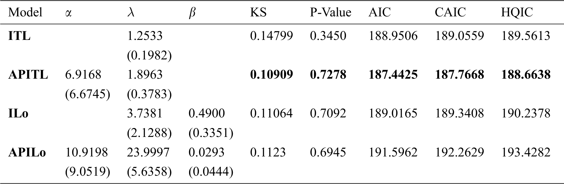
Tabs. 4–6 provide values of Akaike information criterion (AIC), corrected AIC (CAIC), Hannan-Quinn information criterion (HQIC), and Kolmogorov- Smirnov (KS) statistic along with its P-value for all fitted models for three real data. In addition, these tables contain the MLEs and standard errors (SEs) (appear in parentheses) of the parameters for the considered models. We compared the fits of the APITL model with the ITL, IW, APIW, ILo, APILo, IEx, and APIEx models (see Tabs. 4–6). The fitted APITL PDF, CDF, PP-plot and QQ-plot of the three real data were displayed in Figs. 4–6, respectively. These figures indicated that the APITL distribution has the smallest values of AIC, CAIC, HQIC, KS and the largest P-value among all fitted models.

The first (I) set of data was studied in Bjerkedal [24]. It represents the rth survival times (in days) of 72 guinea pigs infected with virulent tubercle bacilli. These data were analyzed in Refs. [25,26]. Tab. 4 listed values of MLEs and statistic measures for data I. Fig. 4 provided estimated PDF, CDF, PP-plot, and QQ-plot of APITL distribution for data I.

The second (II) set of data represents the active repair times (hr) for an airborne communication transceiver [27]. The data are as follows: 0.50, 0.60, 0.60, 0.70, 0.70, 0.70, 0.80, 0.80, 1.00, 1.00, 1.00, 1.00, 1.10, 1.30, 1.50, 1.50, 1.50, 1.50, 2.00, 2.00, 2.20, 2.50, 2.70, 3.00, 3.00, 3.30, 4.00, 4.00, 4.50, 4.70, 5.00, 5.40, 5.40, 7.00, 7.50, 8.80, 9.00, 10.20, 22.00 and 24.50. The MLEs and statistic measures for data II listed in Tab. 5. Fig. 5 provided estimated PDF, CDF, PP-plot, and QQ-plot of the APITL model for data II.

The third (III) set of data was studied in Aarset [28]. It refers to 30 failure times of air-conditioning system of an airplane. Tab. 6 listed values of MLEs and statistic measures for data III. Fig. 6 provided estimated PDF, CDF, PP-plot and QQ-plot of the APITL for data III.

Table 4: MLEs, SEs, and statistic measures for data I

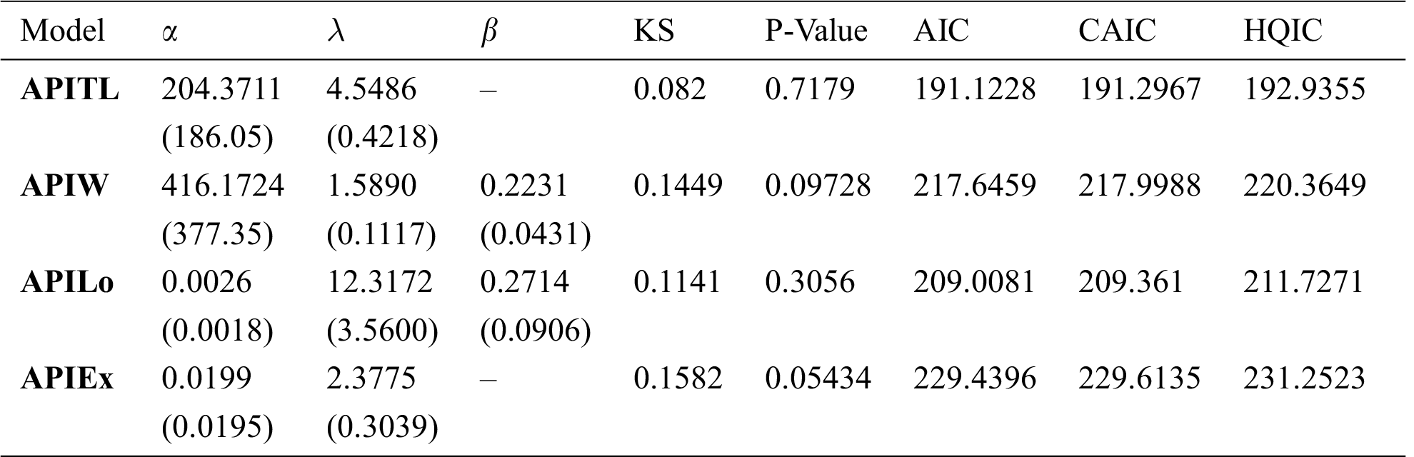
Figure 4: Estimated PDF, CDF, PP-plot and QQ-plot of the APITL model for data I

Figure 5: Estimated PDF, CDF, PP-plot, and QQ-plot of the APITL model for data II

Figure 6: Estimated PDF, CDF, PP-plot, and QQ-plot of the APITL model for data III

Table 5: MLEs, SEs, and statistic measures for data II

According to tables and Figs. 4–6, we observed that the APITL distribution provides well overall the fitted model and consequently could be selected as the more suitable model than other models.

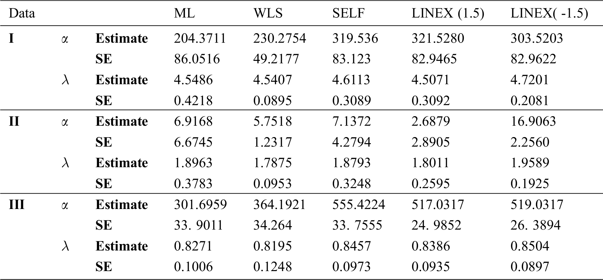
Furthermore, the suggested methods of estimation (see Section 4) for the APITL parameters were considered based on the three data. Tab. 7 displayed different estimates of the APITL parameters for the three data sets. In these data, we cannot use the MPS method because there are equal observations in the data and consequently the spacing followed by the product will be zeros. For more information about this method see [29,30].

Table 6: MLEs, SEs, and statistic measures for data III

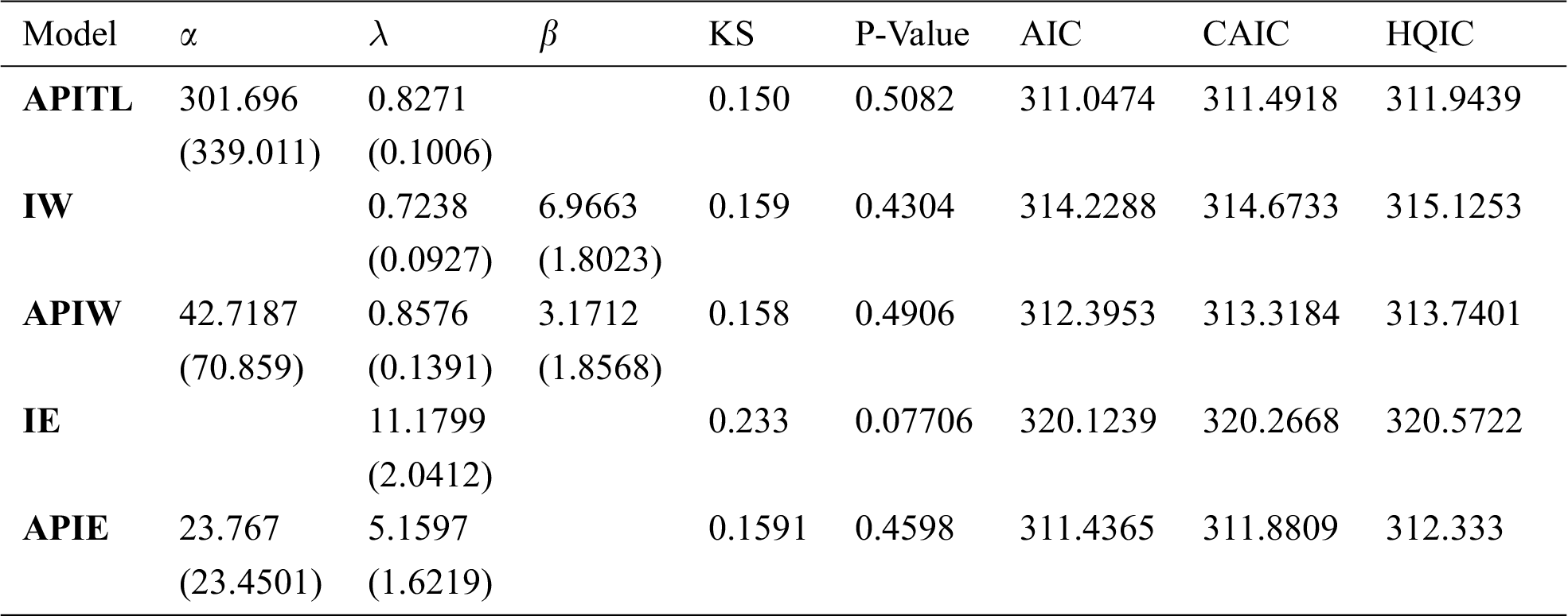
Table 7: Different estimates of the APITL parameters for real datasets

The convergence of the MCMC estimation of α and λ are shown in Figs. 7–9 for all datasets, respectively.

Figure 7: Convergence of the MCMC estimation of α and λ for data I

Figure 8: Convergence of the MCMC estimation of α and λ for data II

Figure 9: Convergence of the MCMC estimation of α and λ for data III

7  Concluding Remarks

We proposed and studied the alpha power transformed inverted Topp-Leone distribution. Some structural properties of the APITL distribution were provided. Bayesian and non-Bayesian methods of estimation were considered. We obtained the ML, WLS, and MPS estimators of the population parameters. The Bayesian estimator was deduced under LINEX and SELF. The Monte Carlo simulation study was worked out to assess the behavior of estimates. Generally, we concluded that the Bayes estimates are preferable to the corresponding other estimates in approximately most of the situations. We proved empirically that the APITL model reveals its superiority over other competitive models for different real data.

Acknowledgement: Thank a lot for every one help full.

Funding Statement: The authors received no specific funding for this study.

Conflicts of Interest: The authors declare that no conflicts of interest to report regarding the present study.

This work is licensed under a Creative Commons Attribution 4.0 International License, which permits unrestricted use, distribution, and reproduction in any medium, provided the original work is properly cited.