DOI:10.32604/iasc.2021.018115
| Intelligent Automation & Soft Computing DOI:10.32604/iasc.2021.018115 | |
| Article |
CNN-Based Voice Emotion Classification Model for Risk Detection
1Contents Convergence Software Research Institute, Kyonggi University, Suwon-si, 16227, Korea
2Department of Computer Science, Kyonggi University, Suwon-si, 16227, Korea
3Division of AI Computer Science and Engineering, Kyonggi University, Suwon-si, 16227, Korea
*Corresponding Author: Kyungyong Chung. Email: dragonhci@gmail.com
Received: 25 February 2021; Accepted: 06 April 2021
Abstract: With the convergence and development of the Internet of things (IoT) and artificial intelligence, closed-circuit television, wearable devices, and artificial neural networks have been combined and applied to crime prevention and follow-up measures against crimes. However, these IoT devices have various limitations based on the physical environment and face the fundamental problem of privacy violations. In this study, voice data are collected and emotions are classified based on an acoustic sensor that is free of privacy violations and is not sensitive to changes in external environments, to overcome these limitations. For the classification of emotions in the voice, the data generated from an acoustic sensor are combined with the convolution neural network algorithm of an artificial neural network. Short-time Fourier transform and wavelet transform as frequency spectrum representation methods are used as preprocessing techniques for the analysis of a pattern of acoustic data. The preprocessed spectrum data are represented as a 2D image of the pattern of emotion felt through hearing, which is applied to the image classification learning model of an artificial neural network. The image classification learning model uses the ResNet. The artificial neural network internally uses various forms of gradient descent to compare the learning of each node and analyzes the pattern through a feature map. The classification model facilitates the classification of voice data into three emotion types: angry, fearful, and surprised. Thus, a system that can detect situations around sensors and predict danger can be established. Despite the different emotional intensities of the base data and sentence-based learning data, the established voice classification model demonstrated an accuracy of more than 77.2%. This model is applicable to various areas, including the prediction of crime situations and the management of work environments for emotional labor.
Keywords: Convolutional neural networks; machine learning; deep learning; voice emotion; crime prediction; crime prevention; IoT
With the development of the Internet of things (IoT) and artificial intelligence (AI), techniques for the convergence of IoT devices and AI have expanded to various areas. These techniques have also been applied in criminal science. Accordingly, the reduction of crimes has been investigated using such a technology [1]. IoT devices for crime prevention include closed-circuit television (CCTV), drones, and wearable devices. Among them, smart CCTV is widely applied in combination with various auxiliary functions, such as behavior recognition and face recognition, for follow-up measures against crimes and crime prevention. CCTV systems have been rapidly developed from analog CCTVs capable of only recording videos to network-based smart CCTV systems [2]. In particular, smart CCTV interacts with various auxiliary functions, such as behavior recognition and face recognition. Accordingly, diverse measures for crime prevention, such as a method for recognizing law-breaking actions and sending a signal to a control system, or a method for installing a speaker and ringing an alarm in case of expected crime, have been developed [3]. In addition, CCTV has been applied to image recognition technologies, such as intrusion detection and tracking, and to various video surveillance systems, such as traffic control systems [4,5]. Accordingly, it has been applied in diverse fields, including disaster prevention, traffic control, and crime prevention and investigation. CCTV has been widely employed globally for crime prevention, irrespective of criticisms regarding privacy violations. These IoT devices have some limitations: as they generate life-logs, they can cause privacy violations. Furthermore, video supervision cameras and network equipment are relatively expensive. In addition, significant errors are likely to occur depending on the recognition range of the camera and the external environment. Therefore, this paper proposes a danger detection classification model using a microphone sensor that has a low range of privacy violations and a wide range of data collection. The proposed model classifies personal emotions based on the vocal frequency input from a microphone sensor. The classified data can be used to predict criminal actions based on emotions, such as anger or fear, generated before or after criminal actions. Recently, voice-based studies have employed speech recognition technology. Such studies focus on the machine analysis of speech language and conversion into text data. These studies facilitate the delivery of commands or information between humans and machines through IoT sensors. Recently, a pattern matching method based on sufficient data that has a high accuracy and supports personalized service through smartphones or separate terminal devices has been investigated. To classify voice data for crime prediction, specific patterns, such as intonation and exclamation, need to be recognized, rather than the implications of voice. Previous studies are not appropriate for the analysis of dangerous situations. In this study, short-time Fourier transform (STFT) [6] and wavelet transforms [7,8] are used as effective acoustic preprocessing techniques to create a frequency power spectrum [9] as an image. These transforms are combined with a residual network (ResNet) [10] based on a convolutional neural network (CNN) [11,12], which is a typical artificial neural network algorithm for image classification. In this process, the auditory frequency pattern is confirmed explicitly through the selection of a gradient descent and the use of a feature map, and the accuracy is improved. By expanding the acoustic IoT model, the limits of the field of view of the visual IoT system, such as smart CCTV, environmental (seasons and weather) limits, and day- and night-time accuracy deterioration may be overcome. In particular, as the proposed model supports inexpensive mass establishment, such devices may be attached to urban facilities, such as streetlights and utility poles. In addition, when these devices are installed in external environments, crimes can be detected in a similar way to CCTV in terms of situational crime prevention, and a large secondary effect may be expected.
2.1 IoT-Based Crime Prevention
IoT technologies including CCTV, drones, big-data analysis, AI, and smart devices have been rapidly developed in recent times. Accordingly, studies have been conducted to respond to various types of crimes in dead zones by applying IoT technologies [1,13]. The convergence techniques of IoT devices and AI facilitate crime prevention and prediction beyond follow-up measures and punishment for crimes [14,15]. CCTV is a typical IoT device used for crime prevention. It supplements the limited manpower and budget of the police. In addition, it supports immediate responses to crime situations. Above all, CCTV can aid in crime prevention; furthermore, it can record crime situations, and the recorded data can be used to arrest criminals [1]. CCTV supports the “situational crime prevention theory” through which the possibility of crime can be reduced in terms of the “rational choice theory” and “opportunity model” [16]. According to the rational choice theory, crimes are reduced when the crime-induced earnings are lower than the crime-induced danger. In the opportunity model, whether to commit a crime depends on the situation, and thus, surveillance factors, such as place and time, need to be enhanced [17]. CCTV helps reduce crimes. However, it has a greater influence on misdemeanors than on felonies [18].
AI technology can recognize big-data patterns for crime analysis using an intelligent algorithm. By extracting significant amounts of data, it can provide data to prevention organizations, such as control centers, and organizations for follow-up measures, such as policy agencies. Accordingly, an AI system requires a machine-learning algorithm that can analyze a large amount of data accurately and efficiently. Today, machine-learning algorithms are widely applied, as they can effectively analyze not only various log files (internet access, credit card purchase records, etc.) but also unstructured data (documents, voices, videos, etc.) [2,19]. The most typical unstructured type of big data used for crime prevention is video information from CCTV cameras. CCTV combined with smart video analysis technology is called smart CCTV [2], and it is capable of analyzing video information in real time and detecting specific abnormal behaviors [2,20,21].
Predictive policing (PredPol) [22] is a representative crime big-data analysis technique. It is the most generally used predictive policing algorithm in the US. Based on AI, PredPol predicts places and time slots with high possibilities of crime in real time. CrimeScan, a predictive crime response program developed after PredPol, predicts various types of crimes by using diverse data, including Facebook data, 911 telephone logs, and police reports. This program has been used in various countries.
The combination of IoT and big data effectively responds to various crimes. Nevertheless, the life-logs generated by IoT devices, such as wearable devices and CCTV, can cause privacy violations. Therefore, rational guidelines must be established to harmonize usefulness and the infringement of personal information [2]. In particular, CCTV has legal issues with traditional confiscation and search, and the collected CCTV data belong to the scope of the search. Therefore, an appropriate compromise between the common good of the majority and the privacy and freedom of individuals needs to be established. In addition, not only base big data, but also data reprocessed through AI technology can be reused for crime analysis. Therefore, a legal system related to big-data collection, cleansing, and analysis processes needs to be established. If a decision is made based on AI, intelligent systems have limitations in terms of legal responsibility [2,23]. In particular, as statistical techniques based on data mining and artificial neural networks have no legal and normative grounds, the limitation of legal responsibility for algorithms and users is unclear. The content for the analysis of algorithm operations, such as eXplainable AI (XAI), needs to be included to enhance the transparency of the decision-making results of algorithms. This content helps secure procedural legitimacy in predicting the outcome of a decision-making system. Therefore, there is an opinion that it is reasonable to define legally the offering of the analyzed content of the outcome of the decision-making system [2].
2.2 Voice-Recognition-Based Classification of Emotions
Speech recognition technology has witnessed significant progress with the development of sensing technology and deep learning. Speech is the easiest way to communicate. Speech recognition technology is capable of interpreting human speech language in machine language and processing it as text data (called speech to text). This technology facilitates easy and convenient human–machine communication [24]. A case in point is the hidden Markov model (HMM) algorithm. Markov models refer to the probability models of changes in certain phenomena. The HMM algorithm is an expansion of the Markov model with hidden states and direct observations [25]. HMM-based speed recognition estimates the parameters of a model using speed signals. Accordingly, the process of determining the similarity to the pattern of input speech can be defined. This method shows an excellent performance if there is a sufficient amount of data for model training. Therefore, it is used as a pattern search method for speech recognition. In a statistical language model, speech and language processes can be developed through a single structure [26]. For instance, people can communicate with their smartphones easily through Samsung’s Bixby [27], Apple’s Siri [28], and LG’s ThinQ [29], and they can receive personalized services.
The intonation, volume, and vibration of people’s voices may vary depending on the context. Accordingly, emotional changes can be judged. Therefore, studies have been actively conducted to find the emotional state of a person and recognize his/her emotions through a pattern analysis of the vibration, pitch, or other types of voice information [30]. Law et al. [30] proposed an automatic voice emotion recognition method in parent–child conversations. The proposed method uses a support vector machine to improve the accuracy of automatic speech recognition to analyze a conversation between a parent and a child in their everyday life. It automatically extracts features from audio signals and labels the minimum or expanded acoustic features extracted with OpenSMILE [31], which is a software application to classify voice and music signals, as small and big speech data. In addition, it analyzes the prevalence of classes with neutral features and addresses the issue of performance optimization of calculation cost in automatic voice emotion recognition and the concept of an emotionally neutral state. Cámbara et al. [32] proposed a convolution speech recognition method using speech quality and the degree of emotion. The proposed method based on CNN has been tested in the framework of automatic speech recognition (ASR) in terms of the degree of emotion and nervousness/shakiness of the voice. During the evaluation, sound quality and the characteristics of sound quality are added to the spectrum coefficients used in an in-depth speech recognition system. The method can easily identify the psychological or functional attributes of speech and improve the ASR performance. Typical video data include audio and images. Accordingly, video data are split into audio and frames, which are preprocessed. In the case of audio data preprocessing, speech signals are presented in a graph of speech pitch. On the other hand, each frame is designed in the case of image data preprocessing. CNN [33] and long short-term memory (LSTM) [34] are used to analyze the features according to the image and voice sequences. Based on the results from the CNN and LSTM, the classification model obtains a result according to each emotion.
3 CNN-Based Voice Emotion Classification Model for Risk Detection
To classify an emotional state based on voice, the size and type of a waveform need to be analyzed, and a technique for learning and distinguishing the differences among anger, pleasure, and ordinary states needs to be applied. The voice emotion classification model consists of three steps: data collection, preprocessing, and artificial neural network learning. Fig. 1 shows the process of the CNN-based voice emotion classification model for risk detection.
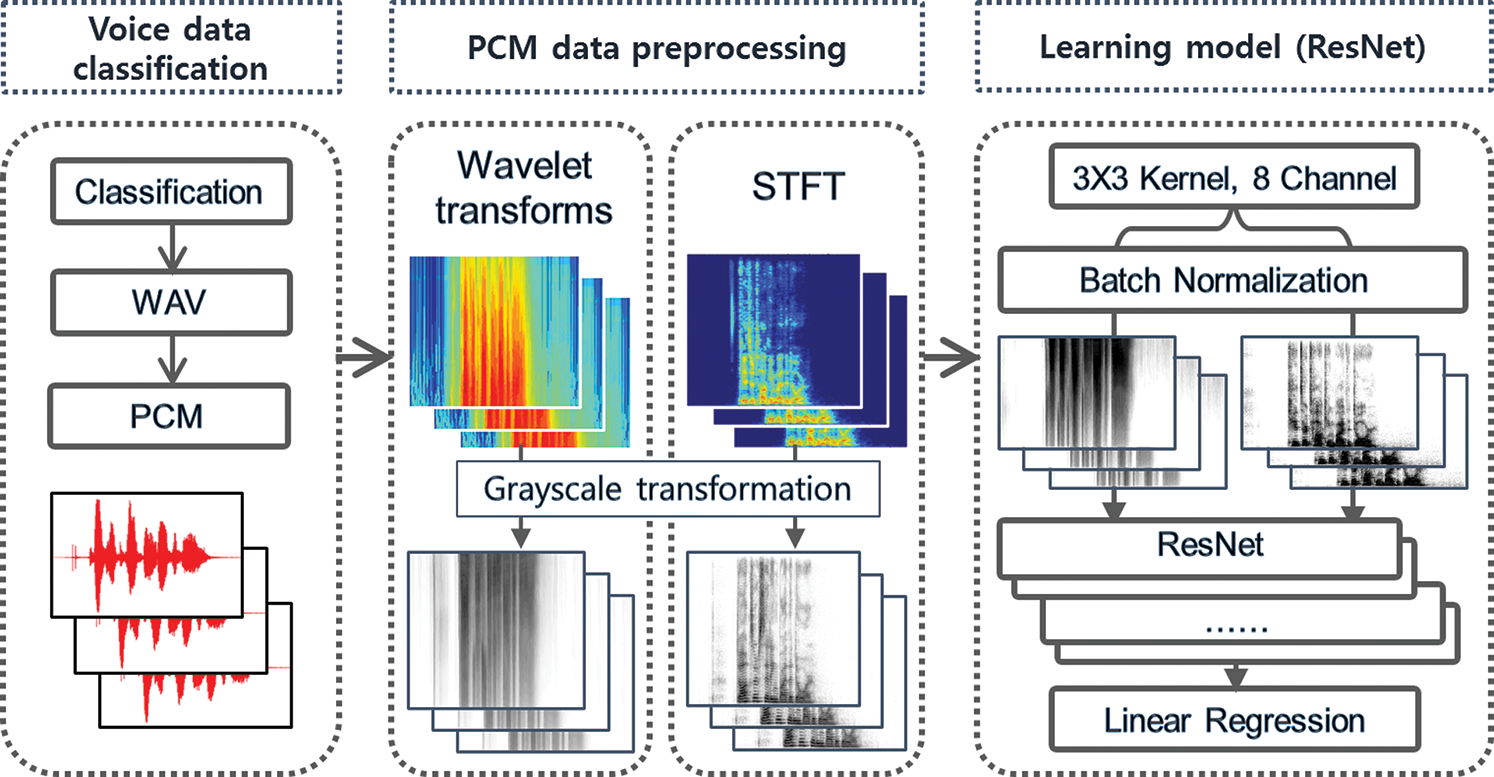
Figure 1: Process of the CNN-based voice emotion classification model for risk detection
In the first step of Fig. 1, the data are collected. That is, voice data are prepared. The voice data are collected as big data from people with various emotions, separated by the type of emotion, and converted into a PCM data format. In the second step, namely preprocessing, the power spectrum is extracted from each of the collected voice files using the STFT and wavelet transforms, and then saved as an image. In the third step, an artificial neural network is established based on the ResNet, and learning is performed based on the two types of preprocessed data. Accordingly, evaluation speed data are added separately, and then, the artificial neural network is implemented.
3.1 Collection and Preprocessing of Voice Big-Data
An artificial neural network algorithm with high accuracy needs to be used [35,36] and uniform and clean voice big-data need to be used for learning, to classify voice big-data effectively. The Ryerson Audio-Visual Database of Emotional Speech and Song (RAVDESS) was used as basic voice data for learning [37]. RAVDESS consists of 7,356 files containing the voice data of 24 professional actors in the categories of calm, happy, sad, angry, fearful, surprise, and disgust expressions. First, the data for learning and evaluation were preprocessed. The number of first audio files was 1,440, and they were classified according to the emotion. In RAVDESS, the number of data points for each emotion is equal, but the neutral data are half in size. Therefore, a class imbalance can occur. Thus, an oversampling technique was applied to solve this problem. Oversampling is the process of applying random-crop to the resulting images of the STFT and wavelet transforms for neutral data. Thus, 96 + 96 data points were obtained for neutral items. Tab. 1 shows the categories of the basic voice data.

In Tab. 1, each emotion has 192 data points, and 1,536 data points are obtained. Among them, 1,120 data points were randomly selected, and 416 data points were used for evaluation. Voice data are composed in the form of frequencies. Therefore, unique features need to be extracted from the saved frequency files, and patterns should be detected. A typical method of presenting frequency characteristics is the Fourier transform, which converts input signals into periodic functions with various frequencies. Using the Fourier transform, the characteristics of the frequency bandwidth can be extracted and noise filtering can be performed. In particular, the Fourier transform is used to reduce data. As it reduces the voice data of the sensor, the complexity of the input layer can be remarkably reduced in the artificial neural network system, thereby significantly decreasing the form and operation amount of the neural network. Fig. 2 shows the results from the PCM and Fourier transform of the voice data files for learning.
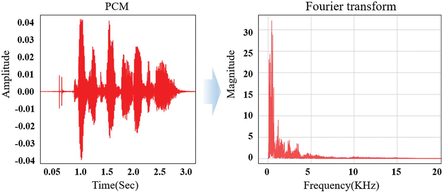
Figure 2: Results from PCM and Fourier transform of the voice data
In the left-side image of Fig. 2, the vertical axis is the amplitude of the voice file PCM for learning, and the horizontal axis represents time. In the right-side image, the vertical axis indicates the magnitude of the frequency of the Fourier transform, and the horizontal axis indicates the frequency. The general Fourier transform fails to detect a change in frequency over time. Thus, STFT, an expanded Fourier transform, or wavelet transforms are used to overcome this problem. STFT divides the entire acoustic data into given short grids, and then applies a Fourier transform to the data in each grid. Thus, it can express the features of the frequency change over time. Although the wavelet transforms are similar to STFT in terms of the basic concept, they lower the frequency resolution of high-frequency signals and decrease the time resolution of low-frequency signals to reduce the data volume. Thus, over time, they can express various frequencies in a 2D image, which is called a spectrogram. Accordingly, using the spectrogram, the change of each wave over time can be determined more effectively. The method proposed in this paper preprocesses data using the STFT and wavelet transforms to clarify the frequency change over time. Through artificial neural network learning with the same structure, this method selects a preprocessing method with a high accuracy between the STFT and wavelet transforms. A discrete Fourier transform (DFT) [6] is used to implement STFT. Generally, if a discrete signal input function is f(x), the DFT is expressed as in Eq. (1).
where N represents the total number of data, and i represents an imaginary number [38]. STFT splits the DFT in a short time unit to extract data, and the extracted data for each frequency are called the power spectrum. These power spectrums are connected with each other, and colors are applied according to the signal intensity; thus, a spectrogram is generated. Fig. 3 shows the spectrogram generated using the STFT.
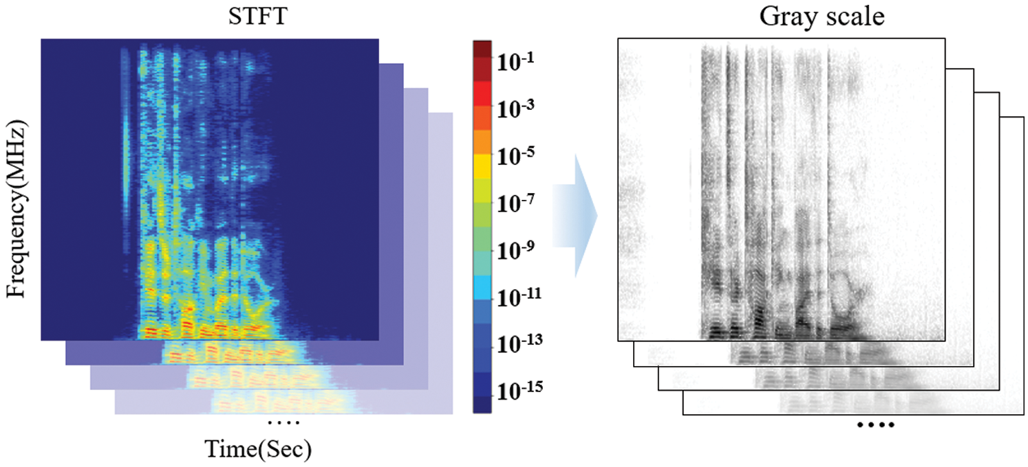
Figure 3: Spectrogram generated using STFT
The spectrogram in Fig. 3 is transformed into grayscale and then used for learning in the artificial neural network to reduce the operation cost. The wavelet transforms use various basic functions that change with each frequency area. A wavelet refers to the repeated increase and decrease in oscillation that begins at zero. Eq. (2) represents a wavelet coefficient that consists of a scale to determine the wavelet size and a translation (trans) related to the time flow [7,8].
where t represents the time.
Accordingly, a wavelet transform function meets the point where random signals are simultaneously limited to one part of the entire time–frequency area [7,8]. In general, a wavelet transform is expressed as in Eq. (3).
In addition, a wavelet transform controls the resolution to improve the resolution over time in a high-frequency area and the resolution of frequency in a low-frequency area. As it controls the resolution according to the number of sound vibrations, the analysis performance can be improved in all frequency areas. Fig. 4 shows the spectrogram generated using the wavelet transforms.
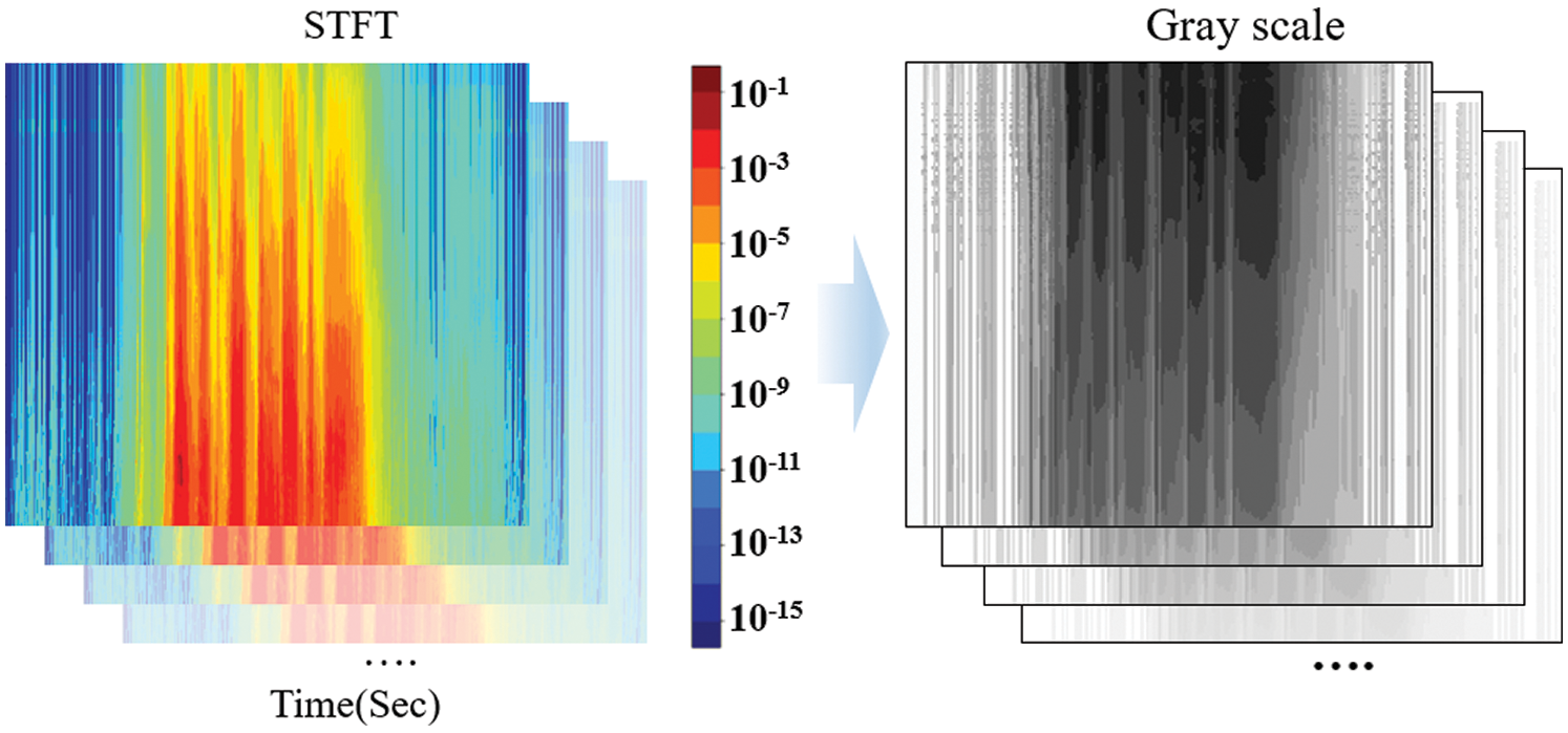
Figure 4: Spectrogram generated using the wavelet transforms
Fig. 4 shows the spectrum image generated using the wavelet transforms and the image used as an input to an artificial neural network. The image extracted using each preprocessing algorithm was used as the input of an artificial neural network. Each image has a PNG format and a grayscale based on a size of 256
3.2 Emotion Classification Model using CNN-Based ResNet
First, an artificial neural network model appropriate for the input data needs to be established [39,40]. The preprocessed acoustic data were designed as a type of 2D image. Therefore, an effective algorithm for classifying 2D images should be applied. A typical AI algorithm for recognizing a 2D pattern is a CNN that operates effectively for image analysis and voice classification. This study uses the structure of a CNN-based ResNet. The basic structure of an emotion classification model consists of input, hidden, and output layers. The hidden layer uses the structure of ResNet, in which the internal data of a neural network are skipped layer by layer to enhance the output. In the ResNet structure, the problem of vanishing/exploding gradients observed in a general CNN with the increase in layers is solved. A neural network that is internally called a residual block is modularized as a block [10,41]. Accordingly, each block is designed via a batch regularization method by adding an input value to an output. Therefore, ResNet produces the effect of overlapping multiple neural networks. Fig. 5 shows the ResNet structure of the hidden layer in the emotion classification model.
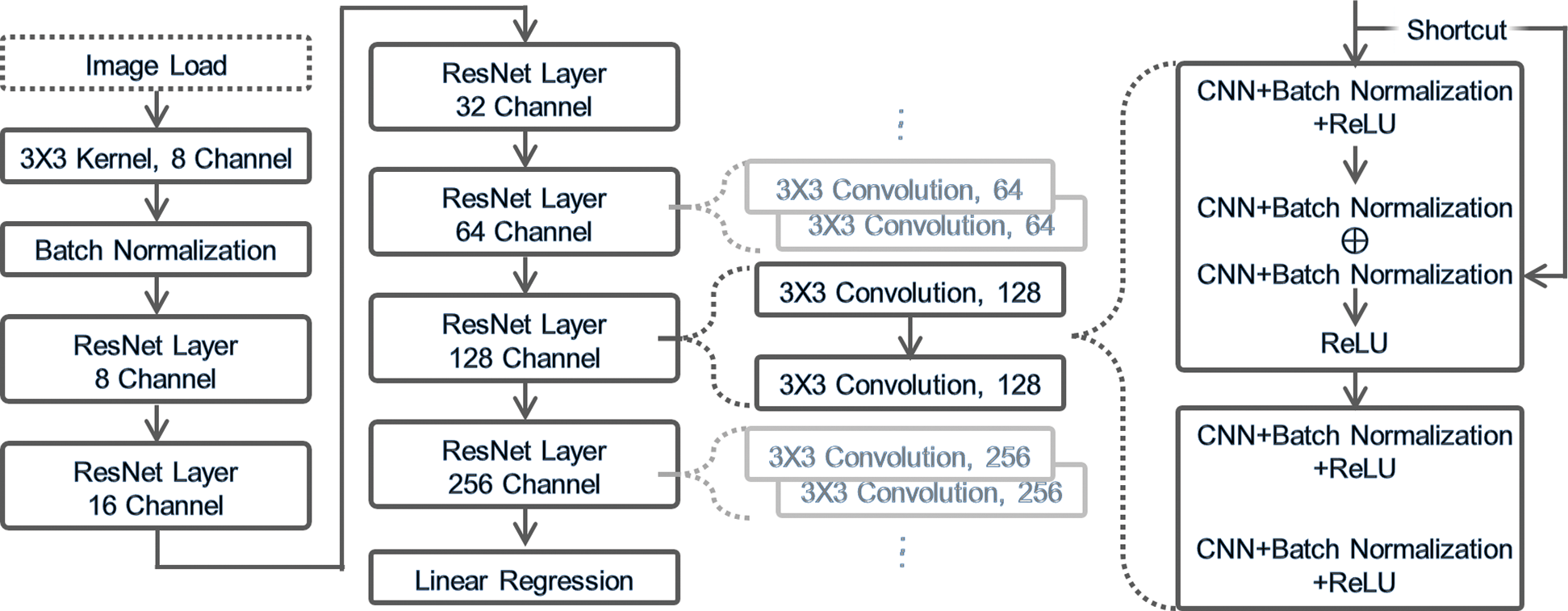
Figure 5: ResNet structure of the hidden layer in the emotion classification model
In Fig. 5, the emotion classification model with the ResNet structure first performs the basic features of CNN, which are the convolution function and batch normalization. Then, it has six layers consisting of residual blocks. In a residual block, an input value repeatedly passes through the next block until the final output node. As types of residual blocks, blocks of tensors with different sizes, that is (8 × 256 × 256), (16 × 128 × 128), (32 × 64 × 64), (64 × 32 × 32), (128 × 16 × 16), and (256 × 8 × 8), exist. Average pooling is applied to the final output value to predict a result.
Training begins with the application of preprocessed data to the input layer of an artificial neural network. Subsequently, feedforwarding is applied to calculate each node-to-node weight and correct errors. Feedforwarding is the process of calculating a weight until an output node passes through all the layers of the artificial neural network. This is called backpropagation. Each node in the neural network requires the selection of a weight control function for the implementation of backpropagation, which is generally called an optimizer. A selected optimizer controls the weight of a node to minimize the error between the output value of the node and the actual value. Stochastic gradient descent (SGD), a typical optimizer, is generally used. In addition, further improved optimizers, such as AdaGrad [42], RMSProp [43], and Adam [44], have been proposed. Adaptive moment estimation (Adam) has the advantages of both Momentum and RMSProp optimizers [45]. This study applies the SGD, which has been improved from Momentum, and Adam, and compares their results. In SGD, in the condition where the weight parameter of the neural network is set as “x,” the result value “f” according to a change in the parameter x is represented as ∂f/∂x, which is a gradient. In SGD, the weight loss function for parameter x is expressed as in Eq. (4) [45].
In Eq. (4), η is the learning rate, which is 0.01 in real learning. As the size of the training data in preparation is small, overfitting needs to be considered. Generally, when the weight is adjusted in SGD, overfitting is avoided by reducing the value by a certain rate. This is called weight decay. The loss function including this rate is expressed as in Eq. (5).
In Eq. (5), λ is the decay rate, which is between 0 and 1. The decay rate used was 0.01. When the weight is updated thus, the previous weight can be reduced by a certain rate. Accordingly, it was possible to prevent a rapid increase in weight. Variables, such as the learning rate and weight reduction, are called hyperparameters. In addition, Adam, as a typical optimizer, is a combination of both Momentum and RMSProp optimizers. Therefore, its equation is formulated as a combination of those of the two optimizers. The Momentum optimizer is an optimizer with the addition of inertia for sliding to a target value [43]. To add inertia, the next sliding vector Mhn+1 is calculated using the equation shown below: Eq. (6) represents the Momentum optimizer.
In Eq. (6),
In Eq. (7), h is an adjustable learning rate; ρ is a hyperparameter (by setting ρ to a small value, a recent gradient can be reflected in a larger way); ⨀ is element-wise multiplication. By assigning a large weight to a recent change amount, a sharp decrease in the learning rate can be prevented. As Adam has a combination of these equations, it is expected to have the advantages of both Momentum and RMSProp optimizers [44].
3.3 Analysis of Internal Spectrum of Emotion Classification Model
After learning an artificial neural network, the performance of the proposed model can be evaluated in terms of accuracy. Nevertheless, it is difficult to determine which pattern in a spectrum is valid for emotion classification. As a secondary algorithm such as XAI is capable of presenting the grounds and reasons for the determination, it can be applied [46,47]. For example, XAI-like local interpretable model-agnostic explanation (LIME) can show the internal operation of an artificial neural network visually [48]. This study expands the concept of LIME and visually implements patterns using a feature map. Thus, the input value of a target image can be inverted sequentially, and the change in the output node in the neural network can be measured [49]. The amount of change made in the process is saved in the feature map, which is finally converted into an image. Consequently, the spectrum patterns of emotions can be expressed visually.
Before analyzing the internal operation of the artificial neural network, a model should be learned completely. A target image was selected for the analysis. After classification, the maximum value of the output node (MaxON) was saved. Each pixel of the target image was inverted sequentially. More specifically, the inversion value of each pixel indicates the farthest number value from an expressible range, and is implemented to have an equal difference. Eq. (8) represents an inversion value ranging from −1 to 1.
With the use of Eq. (8), the target image in which some pixels are inverted is applied to an artificial neural network, and then, the new MaxON value (MaxONnew) is compared. At this time, the positive factor that positively influences the determination made by the neural network is set as PF. Eq. (9) represents the positive factor.
In Eq. (9), the rectified linear unit (ReLu) provides an input value, only if the input value is larger than zero. The generated results were normalized to be presented visually. Subsequently, the brightness level was adjusted. Eq. (10) represents the brightness level adjustment of the pixel values. In the equation, PFmin is the minimum value of PF, PFmax is the maximum value of PF, and
In Eq. (10), the min-max normalization and brightness are adjusted, and thus, a feature map can be observed in an image type. In addition, a change in the predicted output value of the model can be observed with a change in the input value of the artificial neural network. Consequently, the significance can be determined according to the position and form of the acoustic frequency spectrum.
4 Result and Performance Evaluation
An artificial neural network can have different accuracy results depending on the data preprocessing algorithms, layer types, optimizers, and hyperparameters. Therefore, the internal structure should be adjusted and evaluated in various ways. The hardware system used for the evaluation has the following specifications: Intel Xeon Silver 4208 (2.1 GHz) CPU (Intel®, Santa Clara, California, USA) and 16 GB memory. To implement an artificial neural network, this study used Python (Ver 3.8.3), and Spyder4.1.5 was adopted as a development tool. The implementation of ResNet was mainly based on PyTorch (Version 1.6.0). This study used PyWavelets for wavelet calculation and librosa for acoustic data processing and Fourier transform. Additionally, the matplotlib visualization package and numpy package were adopted for numerical calculations. The implemented ResNet artificial neural network learns with preprocessed 1,120 learning data points. The data were processed in a batch unit of 32 data points, and the accuracy was evaluated after 240 epochs. The accuracy of the emotion classification by the proposed model and the accuracy of the wavelet transforms and STFT according to the change in the optimization function are evaluated.
First, the accuracy evaluation of the emotion classification is based on a confusion matrix that shows the rate of prediction by the proposed model as “true” for real truth and as “false” for real false. Tab. 2 lists the confusion matrix used to evaluate the proposed model [38].
Table 2: Confusion matrix for evaluating the proposed model
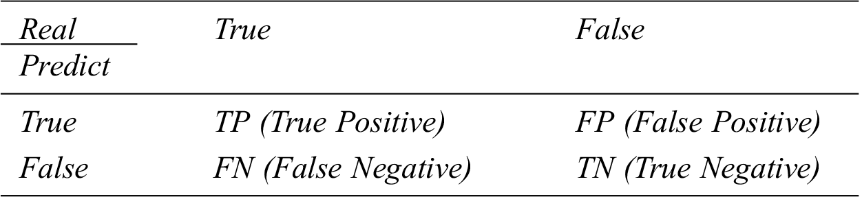
In Tab. 2, TP and TN represent the cases where the predicted values of the proposed mode are correct, and FP and FN represent the cases where the predicted values are incorrect. The calculated accuracy is expressed as in Eq. (11).
In Eq. (11), the accuracy value ranged from 0 to 1. The closer the value is to zero, the lower is the accuracy; the closer it is to 1, the higher is the accuracy.
SGD and Adam are applied to the proposed model to evaluate the accuracy with the change in the activation function. The evaluation was performed with a gradual increase in the learning rate. Fig. 6 shows the evaluation results for the wavelet transforms according to the change in the optimization function. These results are based on the base data and wavelet transforms. SGD and Adam are internally applied to the neural network. The accuracy evaluation result according to the epoch change is shown in the figure.
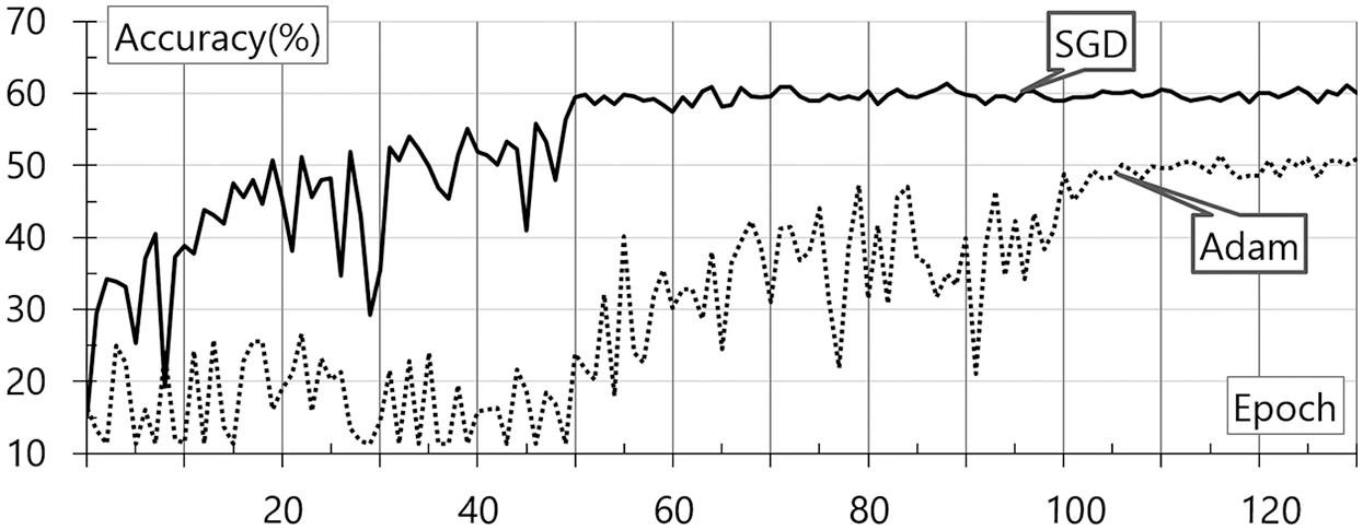
Figure 6: Results of accuracy evaluation for the wavelet transforms according to the change in the optimization function
As shown in Fig. 6, Adam demonstrates a higher accuracy generally. In the case of the voice data to which the wavelet transforms are applied, SGD demonstrates an accuracy of 60% at 50 epochs, showing faster and more accurate results. This result may be attributable to the application of the Momentum optimizer. Nevertheless, this model demonstrates a low classification accuracy of 60%. Fig. 7 shows the evaluation results for the STFT according to the change in the optimization function. These results are based on the base data and STFT. SGD and Adam are internally applied to the neural network. The accuracy evaluation result according to the epoch change is shown in the figure.
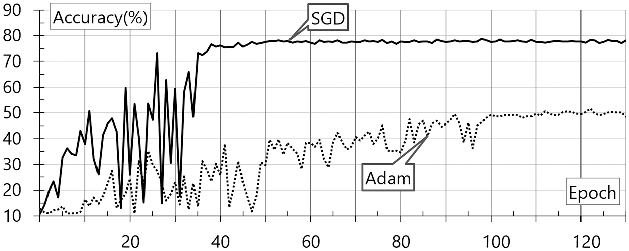
Figure 7: Results of accuracy evaluation for STFT according to the change in the optimization function
As shown in Fig. 7, SGD demonstrates a higher accuracy for STFT. SGD with the Momentum optimizer demonstrates an accuracy of almost 80% after 40 epochs. After 100 epochs, it appears to have a risk of overfitting. Adam demonstrates an accuracy of at least 50% after 120 epochs. Subsequently, overfitting occurs. However, the combination model of the wavelet transforms and Adam demonstrates an accuracy that is lower than expected. Therefore, this aspect should be studied further in a future study. Overall, the SGD combination model with STFT and the Momentum optimizer shows the best accuracy of 77.2% at 57 epochs. This indicates that preprocessing, optimizer selection, and hyperparameter adjustment are important factors.
For the internal analysis of the voice emotion classification model, frequency spectrum patterns were analyzed through a feature map. The STFT data with the best performance were used for the analysis. The artificial neural network learned using SGD was applied. Fig. 8 shows the positive factors that positively influence the determination of acoustic data in the voice emotion classification model.
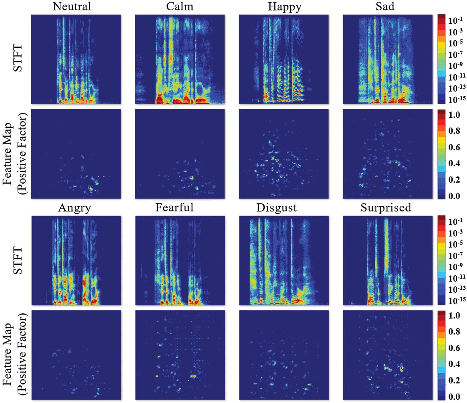
Figure 8: Positive factors that positively influence the determination of acoustic data in the voice emotion classification model
In the top part of Fig. 8, the spectra of voice according to emotional situations are presented. In the bottom part, the pattern recognition factors that are considered important by the artificial neural network according to the emotions in each spectrum are converted into an image. Accordingly, the neural network recognizes different important factors according to emotions and specific patterns can be observed. Thus, it can be visually observed that the voice-based emotions recognized subjectively exist in the frequency and spectrum data, and emotions can be discerned through an artificial neural network.
In this study, artificial neural network algorithms were combined based on acoustic sensor data for crime prevention and prediction. The collected voice data were classified into eight types of emotions. Based on the emotions of anger, fear, and surprise related to dangerous situations, crime situations were predicted. For the implementation of emotion classification, the classified speed data according to emotions were preprocessed using STFT and wavelet transforms. Learning data were expressed as a type of power spectrum image with which a specific emotion pattern was first learned in the same voice scenario. Subsequently, the emotional state of the new voice data was determined. A CNN-based ResNet was applied for the analysis of pattern images. SGD was used as an optimization function for neural network learning in the artificial neural network. For the performance evaluation of the proposed model, the feature map image and accuracy values were compared according to the optimizers. In the learning state of the artificial neural network system from 60 to 80 epochs, the STFT demonstrated a significant accuracy of 77.2%. Thus, the time-based frequency spectrum of STFT includes patterns related to actual emotions and the artificial neural network model correctly classifies patterns. In addition, through a feature map, the patterns of the spectrum related to the emotions generated by the STFT can be visually identified. The results indicate that, for the difficult classification of voice-data-based emotions, the CNN-based artificial neural network can extract association patterns from a spectrum image and classify them.
As the proposed model uses an acoustic module as an IoT sensor, it is less expensive than CCTV and can be used to establish a risk detection system with high accessibility. Above all, it can be free of issues related to the protection of personal information, which have drawn considerable attention recently. To realize this classification model and to implement an immediate response service, a follow-up study with various big data for learning that are classified in smaller units, such as a word or syllable, than a sentence needs to be conducted.
Funding Statement: This research was supported by Basic Science Research Program through the National Research Foundation of Korea (NRF) funded by the Ministry of Education (Grant No. NRF-2020R1A6A1A03040583).
Conflicts of Interest: The authors declare that they have no conflicts of interest to report regarding this study.
1. Y. J. Kim and H. S. Kim, “Safe female back-home system design research in use of situational crime prevention theory-Focusing on IoT technique and drone used possibility of policing,” Journal of the Korean Society of Design Culture, vol. 22, no. 3, pp. 81–91, 2016. [Google Scholar]
2. J. I. Choi, “Current status and limitations of advanced science techniques based on big data analysis-In terms of crime prevention and investigation,” Korean Law Association, vol. 20, no. 1, pp. 57–77, 2020. [Google Scholar]
3. S. Park, M. Ji and J. Chun, “2d Human pose estimation based on object detection using RGB-D information,” KSII Transactions on Internet & Information Systems, vol. 12, no. 2, pp. 800–816, 2018. [Google Scholar]
4. I. F. Ince, M. E. Yildirim, Y. B. Salman, O. F. Ince, G. H. Lee et al., “Fast video fire detection using luminous smoke and textured flame features,” KSII Transactions on Internet & Information Systems, vol. 10, no. 12, pp. 5485–5506, 2016. [Google Scholar]
5. K. Chung and R. C. Park, “P2P-based open health cloud for medicine management,” Peer-to-Peer Networking and Applications, vol. 13, no. 2, pp. 610–622, 2020. [Google Scholar]
6. Q. Zhao, W. Qiu, B. Zhang and B. Wang, “Quickest spectrum sensing approaches for wideband cognitive radio based On STFT and CS,” KSII Transactions on Internet & Information Systems, vol. 13, no. 3, pp. 1199–1212, 2019. [Google Scholar]
7. Z. Liu, L. Li, H. Li and C. Liu, “Effective separation method for single-channel time-frequency overlapped signals based on improved empirical wavelet transform,” KSII Transactions on Internet & Information Systems, vol. 13, no. 5, pp. 2434–2453, 2019. [Google Scholar]
8. H. Liu and X. Zhou, “Multi-focus image region fusion and registration algorithm with multi-scale wavelet,” Intelligent Automation & Soft Computing, vol. 26, no. 4, pp. 1493–1501, 2020. [Google Scholar]
9. S. Hahm and H. Park, “An Interdisciplinary study of a leaders’ voice characteristics: Acoustical analysis and members’ cognition,” KSII Transactions on Internet & Information Systems, vol. 14, no. 12, pp. 4849–4865, 2020. [Google Scholar]
10. K. He, X. Zhang, S. Ren and J. Sun, “Deep residual learning for image recognition,” in Proc. CVPR, Las Vegas, NV, USA, pp. 770–778, 2016. [Google Scholar]
11. H. Li, W. Zeng, G. Xiao and H. Wang, “The instance-aware automatic image colorization based on deep convolutional neural network,” Intelligent Automation & Soft Computing, vol. 26, no. 4, pp. 841–846, 2020. [Google Scholar]
12. G. Choe, S. Lee and J. Nang, “CNN-based visual/auditory feature fusion method with frame selection for classifying video events,” KSII Transactions on Internet & Information Systems, vol. 13, no. 3, pp. 1689–1701, 2019. [Google Scholar]
13. Q. Zhou and J. Luo, “The study on evaluation method of urban network security in the big data era,” Intelligent Automation and Soft Computing, vol. 24, no. 1, pp. 133–138, 2018. [Google Scholar]
14. J. J. Chung, “Application plan by the internet of things for public security policy,” Journal of Police Science, vol. 18, no. 1, pp. 197–228, 2018. [Google Scholar]
15. M. Arif, A. Kattan and S. I. Ahamed, “Classification of physical activities using wearable sensors,” Intelligent Automation & Soft Computing, vol. 23, no. 1, pp. 21–30, 2015. [Google Scholar]
16. A. Crawford and K. Evans, “Crime prevention and community safety,” in The Oxford Handbook of Criminology. Oxford University Press, pp.797–824, 2017. [Google Scholar]
17. T. D. Miethe and R. F. Meier, “Opportunity, choice, and criminal victimization: A test of a theoretical model,” Journal of Research in Crime and Delinquency, vol. 27, no. 3, pp. 243–266, 1990. [Google Scholar]
18. E. H. Park and J. S. Jeong, “The effectiveness of CCTV as the crime prevention policy,” Korean Association of Police Science Review, vol. 16, no. 1, pp. 39–74, 2014. [Google Scholar]
19. B. C. Welsh and D. P. Farrington, “Public area CCTV and crime prevention: An updated systematic review and meta-analysis,” Justice Quarterly, vol. 26, no. 4, pp. 716–745, 2009. [Google Scholar]
20. H. J. Shin and M. J. Kim, “A study on humanities in application of robot technology based on the criminal justice system,” Journal of Korean Public Police and Security Studies, vol. 13, no. 4, pp. 113–134, 2017. [Google Scholar]
21. Z. Yan, Z. Xu and J. Dai, “The big data analysis on the camera-based face image in surveillance cameras,” Intelligent Automation & Soft Computing, vol. 24, no. 1, pp. 123–132, 2018. [Google Scholar]
22. R. Benjamin, “Race after technology: Abolitionist tools for the new jim code,” Social Forces, vol. 98, no. 4, pp. 1–3, 2020. [Google Scholar]
23. Y. C. Young, “A study on criminal liability of artificial intelligence robot and the ‘Human character as personality’ in criminal law,” Journal of Law research. Wonkwang University, vol. 35, no. 1, pp. 95–123, 2019. [Google Scholar]
24. L. Orosanu and D. Jouvet, “Detection of sentence modality on French automatic speech-to-text transcriptions,” Procedia Computer Science, vol. 128, no. 2C, pp. 38–46, 2018. [Google Scholar]
25. Y. Yao, Y. Cao, J. Zhai, J. Liu, M. Xiang et al., “Latent state recognition by an enhanced hidden Markov model,” Expert Systems with Applications, vol. 161, no. 1, pp. 113722, 2020. [Google Scholar]
26. G. Vennila, M. S. K. Manikandan and M. N. Suresh, “Dynamic voice spammers detection using hidden Markov model for voice over internet protocol network,” Computers & Security, vol. 73, no. 2, pp. 1–16, 2018. [Google Scholar]
27. Samsungcom, “BixBy,” samsung.com, 2020. [Online]. Available at: https://www.samsung.com/sec/apps/bixby. [Accessed Feb. 15, 2021]. [Google Scholar]
28. Apple, “Siri,” apple.com, 2020. [Online]. Available at: https://www.apple.com/siri. [Accessed Feb. 15, 2021]. [Google Scholar]
29. LG, “ThinQ,” lge.co.kr, 2020. [Online]. Available at: https://www.lge.co.kr/lgekor/product/accessory/smart-life/LGThinQMain.do. [Accessed Feb. 15, 2021]. [Google Scholar]
30. E. L. C. Law, S. Soleimani, D. Watkins and J. Barwick, “Automatic voice emotion recognition of child-parent conversations in natural settings,” Behaviour & Information Technology, vol. 1, pp. 1–18, 2020. [Google Scholar]
31. Audeering, “openSMILE,” audeering.com, 2020. [Online]. Available at: https://www.audeering.com/opensmile/. [Accessed Feb. 15, 2021]. [Google Scholar]
32. G. Cámbara, J. Luque and M. Farrús, “Convolutional speech recognition with pitch and voice quality features,” arXiv preprint. arXiv2009. 01309, 2020. [Google Scholar]
33. K. Chung and H. Jung, “Knowledge-based dynamic cluster model for healthcare management using a convolutional neural network,” Information Technology and Management, vol. 21, pp. 41–50, 2020. [Google Scholar]
34. D. H. Shin, K. Chung and R. C. Park, “Prediction of traffic congestion based on LSTM through correction of missing temporal and spatial data,” IEEE Access, vol. 8, pp. 150784–150796, 2020. [Google Scholar]
35. J. C. Kim and K. Chung, “Neural-network based adaptive context prediction model for ambient intelligence,” Journal of Ambient Intelligence and Humanized Computing, vol. 11, no. 4, pp. 1451–1458, 2020. [Google Scholar]
36. J. C. Kim and K. Chung, “Knowledge-based hybrid decision model using neural network for nutrition management,” Information Technology and Management, vol. 21, pp. 29–39, 2020. [Google Scholar]
37. S. R. Livingstone and F. A. Russo, “The Ryerson Audio-Visual Database of Emotional Speech and Song (RAVDESSA dynamic, multimodal set of facial and vocal expressions in North American English,” PLoS One, vol. 13, no. 5, pp. e0196391, 2018. [Google Scholar]
38. H. Yoo, “Health big data processing method based on deep neural network for preventing cardiovascular disease,” Ph.D. dissertation. Sangji University, South Korea, 2019. [Google Scholar]
39. J. C. Kim and K. Chung, “Discovery of knowledge of associative relations using opinion mining based on a health platform,” Personal and Ubiquitous Computing, vol. 24, pp. 583–593, 2020. [Google Scholar]
40. J. W. Baek and K. Chung, “Context deep neural network model for predicting depression risk using multiple regression,” IEEE Access, vol. 8, pp. 18171–18181, 2020. [Google Scholar]
41. X. Zhao, W. Liu, W. Xing and X. Wei, “DA-Res2Net: A novel Densely connected residual Attention network for image semantic segmentation,” KSII Transactions on Internet & Information Systems, vol. 14, no. 11, pp. 4426–4442, 2020. [Google Scholar]
42. J. Duchi, E. Hazan and Y. Singer, “Adaptive subgradient methods for online learning and stochastic optimization,” Journal of Machine Learning Research, vol. 12, no. 61, pp. 2121–2159, 2011. [Google Scholar]
43. G. Hinton, N. Srivastava and K. Swersky, “Neural networks for machine learning lecture 6a overview of mini-batch gradient descent,” Cited on, vol. 14, no. 8, pp. 1–31, 2012. [Google Scholar]
44. D. P. Kingma and J. Ba, “Adam: A method for stochastic optimization,”arXiv preprint. arXiv1412.6980, 2014. [Google Scholar]
45. H. Robbins and S. Monro, “A stochastic approximation method,” Annals of Mathematical Statistics, vol. 22, no. 3, pp. 400–407, 1951. [Google Scholar]
46. J. M. Schoenborn and K. D. Althoff, “Recent trends in XAI: A broad overview on current approaches, methodologies and interactions,” in ICCBR Workshops, pp. 51–60, 2019. [Google Scholar]
47. A. Holzinger, “Explainable AI (ex-AI),” Informatik-Spektrum, vol. 41, no. 2, pp. 138–143, 2018. [Google Scholar]
48. T. Peltola, “Local interpretable model-agnostic explanations of Bayesian predictive models via Kullback-Leibler projections,” arXiv preprint. arXiv1810.02678, 2018. [Google Scholar]
49. A. Fisher, C. Rudin and F. Dominici, “All models are wrong, but many are useful: Learning a variable’s importance by studying an entire class of prediction models simultaneously,” Journal of Machine Learning Research, vol. 20, no. 177, pp. 1–81, 2019. [Google Scholar]
 | This work is licensed under a Creative Commons Attribution 4.0 International License, which permits unrestricted use, distribution, and reproduction in any medium, provided the original work is properly cited. |