Intelligent Automation & Soft Computing DOI:10.32604/iasc.2021.017737
Article

Surge Fault Detection of Aeroengines Based on Fusion Neural Network

Desheng Zheng1, Xiaolan Tang1,*, Xinlong Wu1, Kexin Zhang1, Chao Lu2 and Lulu Tian3

1School of Computer Science, Southwest Petroleum University, Chengdu, 610500, China
2AECC Sichuan Gas Turbine Establishment, Mianyang, 621700, China
3Department of Computer Science, Brunel University London, Middlesex, UB8 3PH, United Kingdom
*Corresponding Author: Xiaolan Tang. Email: tangxiaolan1998@gmail.com
Received: 09 February 2021; Accepted: 18 April 2021

Abstract: Aeroengine surge fault is one of the main causes of flight accidents. When a surge occurs, it is hard to detect it in time and take anti-surge measures correctly. Recently, people have been applying detection methods based on mathematical models and expert knowledge. Due to difficult modeling and limited failure-mode coverage of these methods, early surge detection cannot be achieved. To address these problems, firstly, this paper introduced the data of six main sensors related to the aeroengine surge fault, such as, total pressure at compressor (high pressure rotor) outlet (Pt3), high pressure compressor rotor speed (N2), power level angle (PLA), etc. Secondly, aiming at preprocessing of data sets, this paper proposed a data standardization preprocessing algorithm based on batch sliding window (DSPABSW) to build a training set, validation set and test set. Thirdly, aeroengine surge fault detection fusion neural network (ASFDFNN) was provided and optimized to improve the detection accuracy of aeroengine surge faults. Finally, the experimental results showed that the model achieved 95.7%, 93.6% and 94.7% in precision rate, recall rate and F1_Score respectively and consequently it can detect the aeroengine surge fault 260 ms in advance.

Keywords: Sliding window; time series prediction; aeroengine surge fault detection; fusion neural network

1  Introduction

At present, researches on fault detection methods present a trend of diversification. Wu et al. [1] generalized some methods including model-based, knowledge-based, and data-based processing.

1.    Model-based detection. Model-based detection mainly includes two categories. One is based on the failure physics model which is aimed at electronic products. The other is the state space model whose typical representative is fault detection based on random filtering [2–4]. Although these methods can meet the requirements of real-time performance, it is difficult to establish detection models due to complexity and nonlinearity of the engine system.

2.    Knowledge based detection. Knowledge-based detection can give full play to the knowledge and experience of experts in various disciplines of the engine. Therefore, it does not require precise physical models. It mainly includes expert system [5,6] and fuzzy logic [7,8]. However, the fault mode covered by the expert knowledge base is limited, so there are still many problems to be solved in practical application.

3.    Data-based detection. The biggest advantage of data-based detection is that it does not need accurate mathematical or physical models, but it can detect faults by datamining. Fault detection based on machine learning [9–12] and deep learning [13–15] has gradually become the mainstream of current detection methods. In particular, engine fault detection based on deep learning can automatically learn predictive characteristics directly through the constructed model without relying on previous assumptions and raw data. A hybrid depth calculation model (HDC) based on CNN, DNN and LSTM proposed by Chen Z et al. [16] can achieve an accuracy rate of about 83% in aeroengine gas path fault diagnosis.

In this paper, firstly, the training set, validation set and test set are constructed by using a specific data preprocessing algorithm called DSPABSW. The experimental data includes six main sensors related to the aeroengine surge fault, such as total pressure at compressor (high pressure rotor) outlet (Pt3), high pressure compressor rotor speed (N2), power level angle (PLA), etc. Secondly, this paper proposed a fusion for aeroengine surge fault detection neural network (ASFDFNN), which is made up of Seq2Seq, CNN and LSTM models. Seq2Seq, a timing data prediction model based on encoder-decoder structure, was used to predict future sensor data, while CNN and LSTM were used to classify the surge fault and judge whether the output sequence of Seq2Seq has the surge fault. Finally, the experimental results showed that ASFDFNN can detect the surge fault of aeroengines in advance by predicting firstly and then classifying.

2  Related Works

2.1 Long Short-Term Memory

RNN is a class of deep neural network for time series data processing. However, it does not work well in dealing with long-term dependency problems. LSTM [17–19] is a variant model in RNN, and it can forget and retain previous information through input control gate, output control gate and forgetting control gate. As a result, it can analyze long-term dependency problems well and effectively make up for the deficiency of RNN.

The first step of LSTM determines which information can pass through the cell and the decision is controlled by the forgetting gate ft , which is expressed as:

ft=σ(Wf⋅[ht−1,xt]+bf) (1)

where ht−1 and xt represent the previous and current cell output respectively. Wf denotes the weight matrix of the forgetting gate. bf and σ stand for the bias and threshold functions. The function selected by σ is Sigmoid. The value of ft from 0 to 1 given by the whole equation will determine the degree to which the information learned previously is connected to the cell.

The second step is to input new information into the cell, which consists of two parts. The first part is to calculate the value of input gate it by the following formula:

it=σ(Wi⋅[ht−1,xt]+bi) (2)

where Wi is the weight matrix; bi is the bias term; and the function selected by σ is still Sigmoid.

The second part is the candidate cell state Ct~ obtained by tanh activation function, which leads to the following formula:

Ct~=tanh(Wc⋅[ht−1,xt]+bc) (3)

After obtaining the value of forgetting gate ft and input gate it , the previous cell state Ct−1 is multiplied by the former, and the current candidate cell state Ct~ is multiplied by the latter, so the current cell state Ct is obtained. This formula can be described as:

Ct=ft∗Ct−1+it∗Ct~ (4)

where * denotes element multiplication. After obtaining the current cell state Ct , it is output to the output gate Ot , which is represented as:

Ot=σ(Wo⋅[ht−1,xt]+bo) (5)

where Wo is the weight matrix of the output gate and bo is the bias term. The output gate Ot can determine the final output ht of the current cell, which meets the following condition:

ht=Ot∗tanh(Ct) (6)

2.2 Seq2seq Network Model

Both RNN and LSTM mentioned in Section 2.1 are limited to fixed length sequence data only. To generate indefinite length sequence data, Seq2Seq [20] is applied because it adopts encoder-decoder structure, in which CNN, RNN, LSTM or other different models are taken as the hidden layer. In this paper, LSTM is used as the hidden layer.

Taking Seq2Seq of ASFDNN as an example, its working principle is to input a variable length sequence into LSTM layer of the encoder to obtain a two-dimensional fixed length eigenvector and the eigenvector comes from the output of the last cell in LSTM. Then, the eigenvector is input into LSTM layer of the decoder as the input of each cell in LSTM layer. The number of its cells corresponds to the length of the final output sequence. Its specific structure is shown in Fig. 1.

Figure 1: Seq2Seq model structure diagram

2.3 Convolution Neural Network

Convolutional neural network (CNN) is a class of feed-forward neural network, which has been widely used in image classification, positioning, etc. In CNN, a group of one or two-dimensional convolution kernels are used to analyze and extract local features. Since each position of the data will be scanned by the same convolution kernel with fixed weight, so it will be shared to each scanning position. As a result, compared with other neural networks, CNN has smaller parameters and more powerful feature extraction.

CNN is divided into one-dimensional convolution neural network (1D-CNN), two-dimensional convolution neural network (2D-CNN) and three-dimensional convolutional neural network (3D-CNN). 2D-CNN is the most commonly used for image processing, and 1D-CNN [21] is used for time series sensor data in this study.

CNN consists of convolution layer and pooling layer. The convolution layer is applied to perceive and mine the features of the input object and then summarize the local features at a higher level to create feature maps. The pooling layer is applied to down sample the features mined by the convolution layer. Therefore, it can compress the number of data and parameters, reduce overfitting, and increase the fault tolerance of the model. In this paper, 1D-CNN convolution without the pooling layer is used to extract the features of time series data effectively.

The general process of one-dimensional convolution is shown in Fig. 2.

Figure 2: Schematic diagram of 1D convolution process

In the graph, T represents time series data; R represents the matrix of time series data; d represents the depth of the matrix—that is, the feature number of each time point in the time series; And t represents the number of time points contained in the time series. F is the filter of current one-dimensional convolution, and l is the length of the convolution kernel of the current filter. C on the right side of the graph denotes the feature map obtained by one-dimensional convolution, and n stands for the number of filters. Since the convolution is carried out in a “Valid” way, the filter is not filled when it exceeds the matrix range. Therefore, the length of the feature map obtained is t−l+1 .

3  Data Set Preprocessing and Partitioning

3.1 Data Labeling Development Formulation

From the content above, the final output of ASFDFNN is a two-category result of whether the engine has the surge fault. Thus, labeling the real data is the basis for completing the entire model training.

In this study, data labeling development based on the numerical curves of Pt3 and PLA sensors in the engine is presented. Pt3 determines the total pressure at the outlet of the compressor, and PLA reflects the degree to which the throttle lever is manually operated. When the value curve of PLA sensor tends to stabilize, the period of time called fault interval appears, during which Pt3 sensor is undergoing a sudden rise, fall, and severe fluctuation until returning to a stable state. Each time point during the interval is the called the time point of fault, and the rest are the time points under normal state, as shown in Fig. 3 below.

Figure 3: Diagram of judging the initial fault point

3.2 DSPABSW

This paper proposed a data standardization preprocessing algorithm based on batch sliding window (DSPABSW), which preprocesses all data by solving two problems. One is how to intercept the sub-sequence of data set and corresponding label set and the other is how to divide the training set and test set.

The data format used in this study is time series data, which refers to the data collected at different points in time and is used to track change over time. For the model, it is infeasible to put millions of time series data in each group into the model training, so it is indispensable to preprocess the data before training to obtain a fixed length subsequence.

Sliding window algorithm is used to divide the fixed length subsequence and the corresponding label set in the engine sensor dataset. In order to get more training data, this paper set the step size of the sliding window to 1.

The labels in the divided label set correspond to the new series obtained by splicing the predicted sequence data and the historical data. The formulation of new sequence labels is to query the labels of all time points of the sequence in the label set defined in Section 3.1. If there is one or more fault points, the sequence proves to be a fault. But if there is no fault point, the sequence proves to be normal.

When sliding window algorithm is used to obtain subsequence samples, the training set and test set need to be divided. Since time series data is applied in this model training, partitioning is different from the traditional data set. For model training, applying data segmentation firstly and then data scrambling is indispensable to prevent overfitting and increase the robustness of the model. However, due to a high autocorrelation of time series data, the data correlation of adjacent periods is high. If data scrambling is applied firstly, the training set will introduce the future number with later time points. According to this, as shown in Fig. 4 below, although the performance of the trained model in the existing dataset is acceptable, it does not perform well in predicting the real unknown sequence data. The main reason is that the model cannot learn the “future pattern” by using partitioning, which is obviously inconsistent with the training purpose.

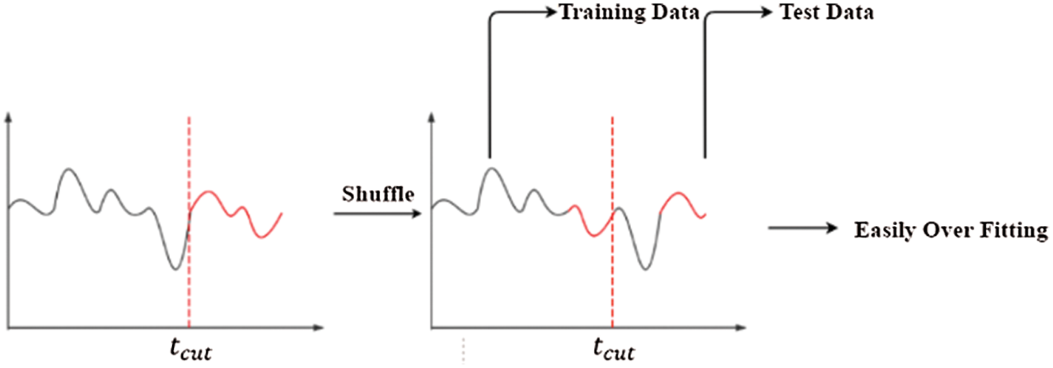
Figure 4: Scrambling sequential data before partitioning dataset

Consequently, sliding window algorithm is firstly used to divide the training set and test set into subsequences. Then one of the time points of the dataset is found according to the partitioning ratio. The subsequences before the time point is the training set, and after that is the test set. The partitioning ratio of the whole dataset is 4:1.

Finally, before model training, the training data and test data need to be standardized to eliminate the errors caused by different dimensions, self-variation or large differences in value. Moreover, it can make the data dimensionless, accelerate the convergence of weight parameters and improve the training effect of the model. This study obtains mean and standard deviation of training set to standardize the training and test sets. If the mean value and standard deviation are obtained based on the whole dataset, the distribution features of future data will be introduced, and the model will also learn the “future pattern”.

The specific algorithm flow is shown in Fig. 5.

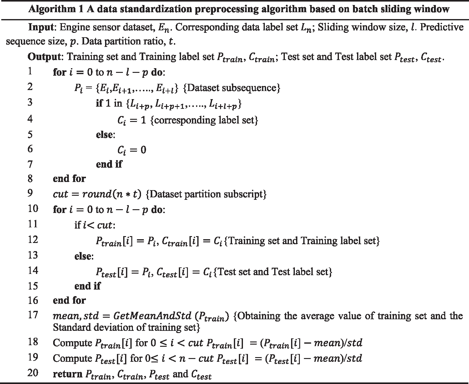
Figure 5: Flow chart of DSPABSW

4  ASFDFNN

The detection of the aeroengine surge fault can be achieved by two steps: the first is to complete multi-dimensional and multi-step prediction on time series multi-sensor data; the second is to determine whether the surge fault has occurred based on the output of the previous step.

In order to complete the steps above, this paper applied fusion neural network for aeroengine surge fault detection called ASFDFNN, which is composed of Seq2Seq, CNN and LSTM. Seq2Seq has the capability to generate specified length sequences data. CNN and LSTM are able to analyze effectively and extract local features, semantic relations and overall trend features of data. They can solve the two problems mentioned above so as to complete prediction firstly and then classification. Thus, it can detect the engine surge fault in advance.

The overall structure of ASFDFNN model is shown in Fig. 6.

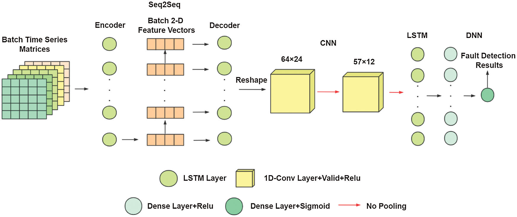
Figure 6: ASFDFNN model structure diagram

From the overall structure, this model structure based on the principle of Occam’s razor is relatively simple. Selecting a suitable and plain model can effectively prevent overfitting. The model is composed of two modules, which complete the two steps of aeroengine surge fault detection respectively. In terms of the specific model structure, the time series matrix of batch number is its input. The first module is a Seq2Seq based on encoder-decoder structure, which is composed of LSTM layers respectively. Its intermediate output is a two-dimensional feature vector of the number of batches, which is the output vector of the last cell in the LSTM layer of the encoder. As for in the decoder, it is the output of the last cell of the encoder. The final result is a prediction sequence with variable length of batch number. Then, a part of the input sequence is spliced with the prediction sequence as the input of the next module, which consists of two one-dimensional convolution layers, one LSTM layer and two fully connected layers. The one-dimensional convolution layer is used to analyze and extract the local features of the input time series data. The LSTM layer is to analyze and extract the semantic relationship between the data in the sequence and the trend features of the whole sequence. The fully connected layer is to transform the sequence information and output the classification with dimension 1.

To get better detection results, it is necessary to select an appropriate activation function to make prediction sequence of the final output in the prediction module as close to the real data as possible. The activation function of the first module does not use Relu function, which is used in the training of the general LSTM layer, because Relu function is too “fragile” and no longer activated for negative output, which leads to a sparse gradient, and thus it is not applicable to all the hidden layers of the model. However, in one-dimensional convolution layer and fully connected layer of the second module, Relu activation function performs well, so it is adopted. The output of the final classification results uses Sigmoid, the function of the output layer of the general binary classification model.

The loss function of the model is defined by the binary cross-entropy function. If the output of the sequence i is a fault. The probability is defined as pi . If the output of the sequence i is normal, the probability is defined as 1- pi . In this case, the expression of loss function L is:

L=1N⋅∑i−[yi⋅log(pi)+(1−yi)⋅log(1−pi)] (7)

where yi is the label value of sample i ; positive class is 1 and negative class is 0.

For higher detection accuracy, this paper removed the pooling layer and set convolution step size to 1 for CNN in ASFDFNN, as shown in Fig. 7 below.

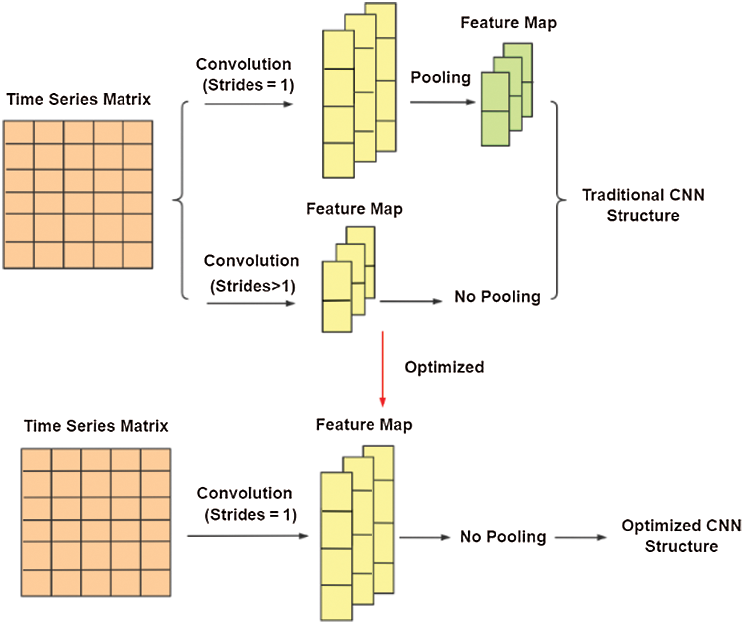
Figure 7: Optimization of ASFDFNN model for CNN

Interestingly, compared with the traditional CNN layer, experimental results showed that the training effect is better after setting convolution step size to 1 and removing the pooling layer. The reason is that although the pooling layer retains the significant features of the convoluted feature map, speeds up the training and reduces over-fitting, it will also lose a lot of information of the feature map. Therefore, this structure does not apply to all data sets. Even if the pooling layer can be replaced by convolution layer with step size greater than 1, the feature information of adjacent time points or pixels will be lost and accordingly the effect is not ideal.

5  Experiment and Results

5.1 Experimental Environment and Data Set

This experiment was mainly carried out under windows 10 operating system and the GPU version was Gtx960m. It applied Python 3.6 as its programming environment and Spyder compiler under anaconda as its programming platform. The neural network was built based on Keras2.2.3 implementation of Tensorflow 1.11.0-GPU.

As for data set, this paper studied 51 groups of sensor data with a total of 300000 pieces obtained from the test under 12 different scenarios such as core engine stall, thrust increase, oil cut-off in inertial start, start-up stall, and compressor distortion, etc.

5.2 Analysis of Test Process

In the experiment, Matplotlib, the python third-party drawing library, was used to visualize the change of loss function in the test process of parameter adjustment. It also should be noted that the training model is based on batch and batch size, which depends on the size of the data set.

As for optimization methods, this paper selected four optimization algorithms: Adadelta, Adam, Adagrad and RMSprop, which are used in most model training for comparison. The cross-entropy curve loss value of the four algorithms is shown in Fig. 8 below.

Figure 8: Comparison of loss curves of different optimization algorithms

The figure above shows that compared with the other three optimization algorithms, RMSprop is the best. Its cross-entropy loss value can be reduced to about 0.03 and the convergence process is more stable. Therefore, RMSprop is selected as the optimization function of ASFDFNN.

The next section of the testing is model algorithm. On the basis of the original model structure, RNN, CNN and LSTM training models are respectively changed for training. Finally, the comparison diagram between cross-entropy loss curve and original model loss curve is shown in Fig. 9 below.

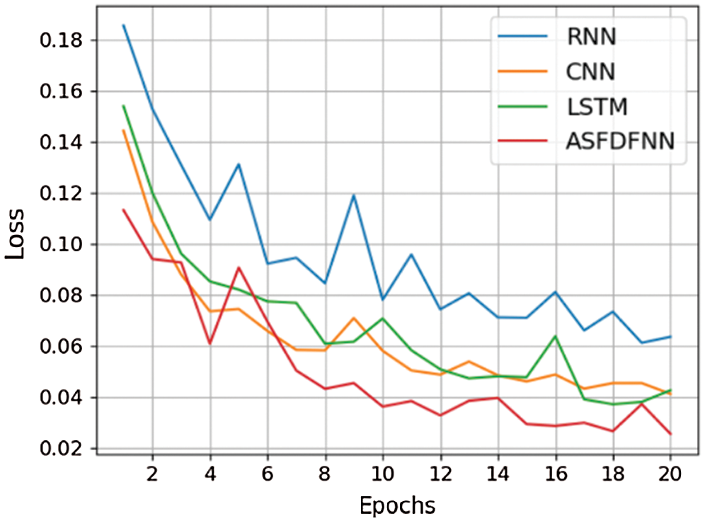
Figure 9: Comparison of loss curves of different algorithm models

It can be seen from the figure above that the loss function convergence of ASFDFNN is faster, and its loss value can decrease to about 0.03, so the training effect is better than other three models.

5.3 Analysis of Test Results

In order to measure the detection accuracy of this model more comprehensively and accurately, this paper selected precision rate, recall rate and corresponding comprehensive evaluation index F1_Score as the final evaluation index of ASFDFNN.

Precision=TPTP+FP×100% (8)

Recall=TPTP+FN×100% (9)

F1_Score=2×Precision×Recall(Precision+Recall) (10)

Taking the model in this paper as an example, where TP represents the number of positive classes predicted as positive classes, while FP represents the number of negative classes predicted as positive classes, and FN stands for the number of positive classes predicted as negative classes. Precision denotes the capability of the model to accurately predict the fault, and Recall signifies the capability to find all surge fault samples. In addition, due to the contradiction between them, the weighted harmonic mean value F1_Score can be calculated to show the overall evaluation of the fault detection capability of the model.

To evaluate the capability of fault detection of ASFDFNN more comprehensively, RNN, CNN and LSTM algorithms were used to test the original model structure. The results of different algorithms were evaluated and compared by three evaluation indexes: precision rate, recall rate and F1_score. The comparison results are shown in Tab. 1.

The table shows that compared with the traditional CNN, RNN and LSTM algorithm for fault detection, ASFDFNN achieved significantly better results.

5.4 Model Time Consuming Assessment

To detect the surge fault of aeroengines in advance, single fault detection of the model should be less than the time span of model detection sequence. In this experiment, as shown in Fig. 10 below, the average time of single fault detection is about 140 ms, and the time span of the detection sequence is up to 400 ms. Accordingly, the model can detect whether the engine has the surge fault 260 ms in advance. In conclusion, the model in this paper can detect the aeroengine surge fault in advance with higher accuracy.

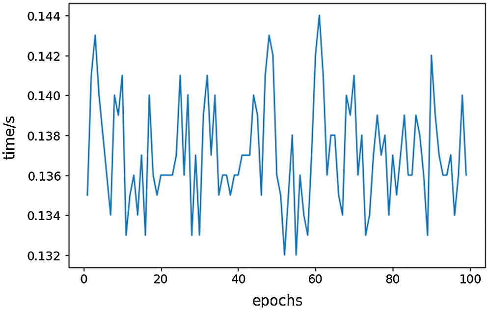
Figure 10: Time consumption curve of ASFDFNN for single fault detection

6  Conclusion

According to preprocessing of aeroengine sensor dataset, this paper proposed a data preprocessing algorithm called DSPABSW to construct a data set and a label set and then applied ASFDFNN for aeroengine surge fault detection. This network consists of Seq2Seq, CNN and LSTM and it can perform early detection of the aeroengine surge fault by predicting firstly and then classifying. The experimental results showed that ASFDFNN can predict the potential surge fault with higher accuracy in a short time.

Funding Statement: This work was supported by Scientific Research Starting Project of SWPU [No. 0202002131604]; Major Science and Technology Project of Sichuan Province [Nos. 8ZDZX0143, 2019YFG0424]; Ministry of Education Collaborative Education Project of China [No. 952]; Fundamental Research Project [Nos. 549, 550].

Conflicts of Interest: The authors declare that they have no conflicts of interest to report regarding the present study.

This work is licensed under a Creative Commons Attribution 4.0 International License, which permits unrestricted use, distribution, and reproduction in any medium, provided the original work is properly cited.